https://doi.org/10.5194/os-15-615-2019
© Author(s) 2019. This work is distributed under the Creative Commons Attribution 4.0 License.
Validation metrics for ice edge position forecasts
Arne Melsom1, Cyril Palerme2, and Malte Müller2
1Research and development department, Norwegian Meteorological Institute, Oslo, Norway 2Development centre for weather forecasting, Norwegian Meteorological Institute, Oslo, Norway
Correspondence:Arne Melsom ([email protected])
Received: 18 December 2018 – Discussion started: 3 January 2019 Revised: 4 April 2019 – Accepted: 6 May 2019 – Published: 29 May 2019
Abstract. The ice edge is a simple quantity in the form of a line that can be derived from a spatially varying sea ice concentration field. Due to its long history and relevance for operations in the Arctic, the position of the ice edge should be an essential element in any system that is designed to monitor or provide forecasts for the physical state of the Arctic Ocean and adjacent ocean regions.
Users of monitoring and forecast products for sea ice must be provided with complementary information on the expected accuracy of the data or model results. Such infor-mation is traditionally available as a set of metrics that pro-vide an assessment of the information quality. In this study we provide a survey of metrics that are presently included in the product quality assessment of the Copernicus Marine Environment Monitoring Service (CMEMS) Arctic Marine Forecasting Center sea ice edge position forecast. We show that when ice edge results from different products are com-pared, mismatching results for polynya and local freezing at the coasts of continents and archipelagos have a large im-pact on the quality assessment. Such situations, which occur regularly in the products we examine, have not been prop-erly acknowledged when sets of metrics for the quality of ice edge position results are constructed.
We examine the quality of ice edge forecasts using a total of 15 metrics for the ice edge position. These metrics are analysed in synthetic examples, as well as in selected cases of actual forecasts, and finally for a full year of weekly forecast bulletins. Using necessity and simplicity of information as a guideline, we recommend using a set of four metrics that sheds light on the various aspects of product quality that we consider.
Moreover, any user is expected to be interested in a lim-ited part of the geographical domain, so metrics derived as domain-wide integrated quantities may be of limited value.
Consequently, we recommend that metrics also be made available for an appropriate set of sub-domains. Furthermore, we find that the metrics decorrelation timescales are much longer than the present forecast range. Hence, our final rec-ommendation is to include depictions of gridded mismatch-ing ice edge positions usmismatch-ing maps for the integrated ice edge error.
1 Introduction
The ice edge location is a primary source of information for safe navigation in ice-infested waters. The retreating sea ice in the Arctic Ocean has given rise to increased naval traffic in the region. The navigation distance from northern Europe to the Far East is about 40 % shorter using the northern sea route when compared to the length of the southern route via the Suez Canal. Hence, commercial shipping is becoming vi-able from an economic perspective due to the changing phys-ical conditions (Ho, 2010; Schøyen and Bråthen, 2011). Our motivation is to provide the increasing number of operators in the Arctic region with easily comprehensible and robust information about the quality of relevant forecasts.
Model results for sea ice concentration are frequently ex-amined by presenting differences from corresponding obser-vations, or results from other models, as shaded contours on maps; see e.g. Johnson et al. (2007) and Arzel et al. (2006). In these and other studies, results for sea ice are often quan-tified by simple statistics for integrated quantities, notably sea ice extent (Massonnet et al., 2012). Statistics for sea ice extent are quantities that can be derived from contingency tables for sea ice concentration categories (Carrieres et al., 2017). A sophisticated approach to examinations of results for sea ice extent has been proposed by Goessling et al. (2016), who introduced the integrated ice edge error (IIEE) as an objective score for differences in the position of the ice edge. An extension relevant for ensemble predictions was re-cently published (Goessling and Jung, 2018). Using this ex-tension, Palerme et al. (2019) find that ECMWF SEAS5 sea-sonal forecasts (Johnson et al., 2019) that are initialised be-tween April and September are more skilful than climatology for forecast ranges of 6–12 weeks.
The fractions skill score (FSS) metric was developed for small-scale features in forecast systems, originally applied to convective precipitation in weather forecasting (Roberts and Lean, 2008). One purpose of the FSS is to provide an objec-tive analysis of how the forecast skill changes as a function of horizontal scales, which is potentially relevant for skill as-sessments of the ice edge position. The FSS was designed for features whose spatiotemporal evolution cannot be fore-casted exactly but rather in a statistical sense.
The present examination of validation metrics for the ice edge position has been performed with the aim of improv-ing information on product quality for users of the products available from the Copernicus Marine Environment Moni-toring Service (CMEMS). CMEMS is the marine compo-nent of the European Union’s Earth Observation Programme. CMEMS has been set up to meet today’s climate and ma-rine challenges by providing the public with observational multiyear and near-real-time products, as well as reanalyses and forecasts from ocean circulation models, sea ice mod-els, wave modmod-els, and biogeochemical models. The informa-tion is integrated into an open and free catalogue of products that is available from http://marine.copernicus.eu/ (last ac-cess: 19 November 2018).
CMEMS is presently organised as 15 production centres, 8 of which process observational data from satellite and in situ platforms, and the remaining 7 centres run and process results from numerical models. These groups of centres are referred to as thematic data assembly centres (TACs) and monitoring and forecast centres (MFCs), respectively.
One of the TACs is dedicated to observations of sea ice, mainly based on data from satellite-borne instruments. Furthermore, three of the MFC model systems have their ocean circulation model coupled to sea ice models. These are the centres responsible for forecasts and reanalyses in the Baltic Sea (BAL MFC), the Arctic Ocean (ARC MFC), and the global oceans (GLO MFC). Sea ice can also occur
in the Black Sea, but the relevant forecast centre (BS MFC) presently has no sea ice product.
Information about the product quality is available for all CMEMS model products, which is provided as statistics for a variety of metrics calculated by comparing results with ob-servational products. Relevant data for sea ice concentration and the position of the ice edge are available from satellite-borne instruments. In this study we assess the quality of fore-casted ice edge positions using a large number of metrics. The sensitivity of the metrics due to differences in observa-tional products is also considered.
The present examination is organised as follows. In Sect. 2 we introduce the metrics used in our analysis: ice edge dis-placement metrics in Sect. 2.1, IIEE and derived metrics in Sect.2.2, and FSS metrics in Sect. 2.3. Next, an idealised situation is constructed to shed light on situations which lead to large differences between model results and observations; this is explored in Sect. 3. This issue is investigated in the context of sea ice forecasts from CMEMS ARC MFC in Sect. 4, where results for two forecast bulletins with differ-ent error characteristics are presdiffer-ented. Then, results for a full year of sea ice forecasts are given in Sect. 5. These results are discussed in Sect. 6, and our examination concludes with a recommended best practice for the validation of sea ice edge forecasts in Sect. 6.3.
2 Definition of metrics
We consider metrics for offsets in ice edge position between two gridded products, e.g. with one product derived from ob-servations and with the other from simulation results from a numerical coupled sea ice–ocean circulation model. In this section, the two products are referred to asOandM, respec-tively. Below we associate grid cell quantities with lower-case indices and integral properties with upper-lower-case indices. Analogously, we separate Euclidean grid cell distance values and integral distance metrics values by denoting these asd andD, respectively.
Note that in our approach, ice edges are associated with areas due to their composition of sets of grid cells rather than curves. The definitions that lead to edge displacement met-rics below do not directly apply to one-dimensional curves. Several displacement metrics between pairs of curves are given by Dukhovskoy et al. (2015).
2.1 Ice edge displacement metrics
In order to compute ice edge displacement metrics the first step is to find the grid cells which constitute the ice edge in the gridded observations as well as in the model product. Letcbe the sea ice concentration, and letce be the sea ice
cells[i, j]that meet the condition c[i, j] ≥ce∧min c[i−1, j], c[i+1, j],
c[i, j−1], c[i, j+1]< ce (1)
where∧is the logical AND operator. LetEbe the ice edge. Ice edgesEOandEMthen correspond to the set of grid cells eoandemthat are returned by this algorithm step when ap-plied to productsO andM, respectively. We also introduce the coordinate position of grid cell[i, j]as[x, y]; letNO be the number of edge grid cells in product OandNM be the number of cells in productM.
Next, for each edge grid cell in each product, we find the distance to the nearest edge grid cell in the other product. Consider first the distance from an ice edge grid cell[im1, jm1]
in the model product at the coordinate position [xm1, y1m]. Then, the displacement of the observed ice edge from this grid cell becomes
dm1 =min
∀eo∈EO:(xo−xm1)2+(yo−ym1)2 1/2
, (2)
where∀is the FOR ALL operator and[xo, yo]is the coordi-nate position of an ice edge grid cell in the observed product. A variant is to consider any land–ocean boundary grid cell as included in the observed sea ice edge. When adopting this variation we refer to the observational product as EˆO, con-stituted by grid cellseˆo. We note thatEO∈ ˆEO. The corre-sponding displacement becomes
ˆ
dm1 =min
∀ ˆeo∈ ˆEO:
(xˆo−xm1)2+(yˆo−ym1)2 1/2
. (3)
We compute the displacement do1 of a model ice edge from an ice edge grid cell in the observational product analo-gously. This is also done fordˆo1afterEmhas been expanded toEˆmby including all land–ocean boundary grid cells.
We can now define a set of symmetric ice edge position metrics expressed as functions of the edge displacements. Here, a symmetric metric is a parameter whose value is in-dependent of whether the observations or the model products form the base of the analysis. We introduce four such metrics here based on results fordmanddo.
1. The root mean square ice edge displacement is
DIERMS=1
2 1 NO NO X
n=1 (don)2
1/2 + 1 NM NM X
n=1 (dmn)2
1/2 . (4)
2. The average ice edge displacement is
DAVGIE =1
2 1
NO NO X
n=1
don+ 1
NM NM X
n=1
dmn
. (5)
3. The ice edge displacement bias, defined here as positive when the ice edge in the model product is on the open ocean side of the ice edge in the observational product:
1IE=1
2 1
NO NO X
n=1
cm[ino, jon] −ce ||cm[ino, jon] −ce||
don
+ 1
NM NM X
n=1
ce−co[imn, jmn] ||ce−co[imn, jmn]||
dmn
, (6)
where||x||is the absolute value of x, and co andcm are the sea ice concentrations in the observations and model, respectively. Also, [io, jo] and [im, jm] denote ice edge grid cells in the observations and model, re-spectively. One may construct situations in which a de-nominator in Eq. (6) becomes 0. In reality, such cases will be very rare, and most of the time this will occur when edge grid cells in the two products overlap, i.e. dn=0. In these cases, we set the fraction to 0.
4. The extreme ice edge displacement, also known as the Hausdorff distance, is
DIEH =max max(do),max(dm), (7) wheredoanddmare the full sets of gridded displacements as given by Eq. (3).
Finally, substituting displacements d in Eqs. (4)–(7) by
ˆ
d as given by Eq. (3) gives rise to a set of supplementary metricsD\RMSIE ,D\AVGIE ,1dIE, andDdIE
H. We note thatDbIERMS≤ DIERMS.
2.2 IIEE metrics
Recently, the integrated ice edge error (IIEE) has been sug-gested as an alternative approach to quantifying the offsets between two ice edges (Goessling et al., 2016). The IIEE is computed from the area between the ice edges in the two products. For a gridded product with a grid cell sizea, set a+=
a for grid cells wherecm> ce∧co< ce
0 elsewhere a−=
a for grid cells whereco> ce∧cm< ce
0 elsewhere.
(8)
Then, the area where the ice edge position in the model product is on the open ocean side of the observed ice edge is A+=X
A
a+, (9)
whereas the complementary situation with the observed ice edge on the open ocean side of the model edge covers the area
A−=X A
(an illustrated example is provided in Sect. 3). The ice edge here is the perimeter of the sea ice extent area. Thus,A+is the area where the ice extent in the model results overshoots the ice extent in the observations and vice versa forA−.
Two area metrics can then be constructed, as given by Goessling et al. (2016).
1. The integral score is
AIIEE=A++A−. (11)
2. The bias score is
αIIEE=A+−A−. (12)
Note that Goessling et al. (2016) also introduced additional area metrics which are not considered here.
The IIEE metrics defined in Goessling et al. (2016) are all provided for areas of sea ice, while no displacement metrics are introduced. Here, IIEE-based displacement metrics are derived by dividing the IIEE areas by an IIEE characteristic length scale. Below, we introduce two definitions of such a length scale.
Summary statistics in the form of a contingency table pro-vide versatile information for the validation of sea ice con-centration results (Carrieres et al., 2017). After categories have been defined by a set of ranges in sea ice concentration, table cells will give areas with category match-ups. Here it is essential to have the sea ice concentration value that defines the ice edge as a value that separates two categories. The sea ice extent for each product is then found as the sum of the relevant rows and columns, respectively. The differences in sea ice extent (quantitiesA+ andA−) emerge from adding the areas in cells that correspond to categories on different sides of the ice edge in the two products.
2.2.1 Edge-length-based IIEE displacement metrics In order to provide scores that have the same dimension as those produced by the ice edge displacement metrics in Sect. 2.1, we introduce metrics that arise when dividing the area metrics given by Eqs. (11) and (12) with the ice edge length. Presently, the ice edge is given as a set of grid cells that were identified from Eq. (1). For simplicity we consider the case in which the resolution in both horizontal directions is constant and equal, and we write the grid cell size ass.
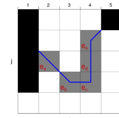
Consider the schematic example provided in Fig. 1. When calculating the length of the ice edge, we must account for the presence of diagonal edge grid cells. This is performed by looping all edge grid cellseand counting the number of[i, j]
edge grid cell neighbours (i.e. among [i−1, j], [i+1, j],
[i, j−1], [i, j+1]) in the same product. If there are two or more neighbours, the edge grid cell contributes with a length le=s (edge grid cellsec, ed in Fig. 1). If there are no such neighbours, the edge length is set to the length of the diagonal, i.e. le=
√
2s (edge grid cell ea). If there is
Figure 1.Schematic illustration for the computation of the ice edge length. The ice edge is displayed by the labelled cells that are filled in gray. Black cells correspond to land. The algorithm we present here for calculation of the ice edge length yields a value that corre-sponds to the length of the blue line; see the text for details.
exactly one such edge neighbour, the contribution becomes le=0.5·(s+
√
2s)(edge grid cellseb, ee). Note that by this definition “open-ended” edge grid cells (e.g. adjacent to land; ea, ee) will contribute with a diagonal representation towards the open end.
The ice edge length in the observational product becomes LO=
X
einEO
loe, (13)
and the corresponding length in the model product is given analogously.
Two length metrics can now be derived from the corre-sponding area metrics.
1. The IIEE average displacement is DIIEEAVG= 2
LO+LM
AIIEE. (14)
2. The IIEE bias is 1IIEE= 2
LO+LM
αIIEE. (15)
2.2.2 Separation-based IIEE displacement metrics An alternative to the application of the scaling length(LO+ LM)/2 in Sect. 2.2.1 is introduced in Sect. S1 in the Sup-plement. The alternative expression for the scaling length is solely dependent on the geometry of the IIEE areas. We then derive a supplementary set of displacement metrics that is analogous to theDIEmetrics defined by Eqs. (4)–(7).
The definitions of metrics in Sect. S1 take dry grid cells adjacent to IIEE areas into account, which the scaling length definition in Sect. 2.2.1 does not. Hence, we adopt the hatted notation as introduced in Sect. 2.1. The resulting displace-ment metrics defined in Sect. S1 are thus denoted asD\RMSIIEE, \
DAVGIIEE,D\IIEE
MAX, and1[IIEE.
2.3 Fractions skill score
We next consider the fractions skill score (FSS), as intro-duced by Roberts and Lean (2008). This metric was defined with the purpose of providing information on the impact of differences on small scales that can appear in results from high-resolution observations and models. The FSS is com-puted for binary results, such as gridded hits and misses due to a criterion, from a pair of products (usually observations and model results). Values for FSS provide information on how the two products compare as a function of resolution. Representations of different resolutions are computed by in-tegration onto coarser (larger) grid cells, and the binary re-sults on the original grid become hit fractions on coarser grids. The FSS reaches its maximum value of 1 at resolu-tion(s) at which representations of the two products are iden-tical and has a minimum value of 0 when no grid cells have overlapping non-zero values.
In the present context, we define hits as grid cells which are part of the ice edge as defined by Eq. (1) in both products. The probability of a grid-cell-by-grid-cell match-up of the edge positions is expected to be reduced when the resolution is enhanced.
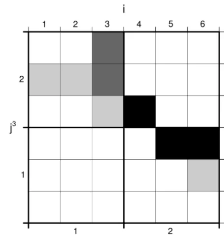
The presentation of FSS in this section is largely based on the Roberts and Lean (2008) article, adapted to representa-tion of lines of grid cells rather than areas. We provide a rele-vant schematic example as Fig. 2, and we use this to illustrate some of the quantities that are introduced below.
Recall from Sect. 2.1 that we identified the sets ofNOand NMgrid cellseoandemthat constitute the ice edgesEOand EMin productsOandM, respectively. We construct a binary gridded representation of the ice edge in productOas
λo[i, j] =
1 ∀eo∈EO
0 elsewhere (16)
so thatP
λo=NO. The corresponding binary representation of the edge in productM,λm, is defined analogously. Next, for productOwe introduce the coarse grid cell ice edge
frac-Figure 2.Schematic illustration for the computation of the fractions skill score for gridded contour lines. Gridded lines representing the ice edge of the model product and the observational product are shown as light gray boxes and dark gray boxes, respectively. Grid cells in which the two lines overlap are black. The original grid is displayed by thin grid lines withx-axis indices at the top andy -axis indices to the right. Thick grid lines correspond to the grid of a neighbourhood with an extent of three grid cells (n=3), withx -andy-axis indices at the bottom and to the left, respectively. See the text for details.
tion for a neighbourhood with an extent ofngrid cells as
λno[in, jn] = 1
n2 n−1
X
k=0 n−1
X
l=0
λo h
in+k−n−1
2 , jn+l−n−1
2 i
, (17)
wherenis an odd number. Again, we defineλnmanalogously, and we note thatλo=λ1o. In the example in Fig. 2, a neigh-bourhood extent of three grid cells is indicated by the thick grid lines, and for this case we find
λnO=3=1
9
2 1 0 2
; λnM=3=1
9
3 1 0 3
. (18)
The mean square edge fraction error for a neighbourhood extent ofngrid cells becomes
MSEn= 1
Nn xNyn
Nxn X
in=1 Nyn X
jn=1 h
λnm[in, jn] −λon[in, jn]i2, (19)
MSE value as the largest possible with the present extent of the edge grid cells.
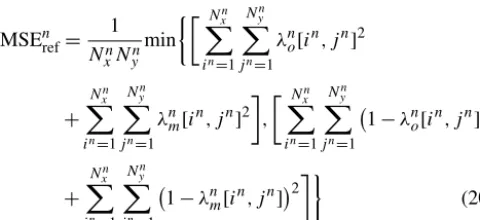
MSEnref= 1
Nn xNyn
min Nxn
X
in=1 Nyn X
jn=1
λno[in, jn]2
+ Nn
x X
in=1 Nyn X
jn=1
λnm[in, jn]2
,
Nxn X
in=1 Nyn X
jn=1
1−λno[in, jn]2
+ Nn
x X
in=1 Nn
y X
jn=1
1−λnm[in, jn]2
(20) This expression is a worst-case arrangement of hits and misses that takes into account situations in which hits out-number misses. This is a modification of the corresponding definition in Roberts and Lean (2008), whose Eq. (7) allowed for situations with MSEnrefexceeding 1.
For the skill score with the original 6×6 grid in Fig. 2 we have MSEn=1=6/62 and MSEnref=1=12/62, while for the n=3 neighbourhood displayed by the thick grid lines we have MSEn=3=2/(2·9)2and MSErefn=3=9/(2·9)2.
Now, the resolution-dependent fractions skill score is in-troduced as
FSSn=1− MSE n
MSEnref, (21)
which has a value of 1 for a perfect forecast for neighbour-hood extentn(λnm=λno∀in, jn⇒MSEn=0) and a value of 0 when λnm·λno=0∀in, jn (⇒MSEn=MSEnref). Note that invoking the modified definition of MSEnrefin Eq. (20) makes the FSSn metric symmetric in the sense that reversing the definition of hits and misses does not affect the FSSnscore.
For the sample case in Fig. 2 we then find that FSSn=1=
1/2, and for then=3 neighbourhood displayed by the thick grid lines we have FSSn=3=7/9≈0.78.
Moreover, we note from Eqs. (19)–(21) that the FSS score will not change if we introduce a set of additional grid cells in which neither product has an ice edge, provided that non-events dominate non-events (i.e. the first term in Eq. (20) is used; here meaning that the number of nodes without an ice edge is larger than the number of edge nodes). This observation has consequences for two different aspects in the present study.
First, when modelling the ocean, dry nodes are usually not considered to be part of the computational domain and are as-signed a special value in numerical results. When integrating over a neighbourhoodn >1 one option would be to discard the grid cells that are dry in the original representation. We will then be left with a result which has a non-constant neigh-bourhood size withn2if dry nodes are not present and< n2 for neighbourhoods in which dry nodes are present. Here, we choose to avoid the problem of non-constant neighbourhood sizes by adoptingλo=λm=0 for dry grid cells.
Second, the grid forn=3 indicated by thick lines in Fig. 2 is only one of nine possible configurations. Since the FSS re-sults are not affected by additional grid cells in which neither
product has an ice edge, we can expand the original domain by adding a padding region ofn−1 grid cells. In the case ofn=3 all configurations are attained by shifting the neigh-bourhood by zero, one, and two original grid cells in both directions. The average FSS score from all of the configu-rations will be used henceforth in this article, since the al-ternative is a set of results that will depend on an arbitrary configuration subset choice.
As an expansion of the FSS metrics, Skok and Roberts (2018) introduced the FSS displacement, which we will refer to asDFSS. An initial estimate forDFSSis derived by first determining for which neighbourhood size the FSS exceeds 0.5. The full algorithm for computing this displacement met-ric is given at the end of Skok and Roberts (2018) and is not repeated here. In most cases DFSS will become about half of the minimum metric neighbourhood size at which the FSS exceeds 0.5. The reliability ofDFSSdecreases when the frequencies are biased (Skok and Roberts, 2018). Here, this translates to differences in the number of ice edge grid cells in observations and in the forecast. In the present study we implement a reduction of the product with the longest ice edge by randomly removing ice edge grid cells from this product. Thus, an unbiased version of the two grid cells is used when computingDFSS. The random removal of grid cells is repeated a number of times, and the average value of the resulting displacements is taken to represent theDFSS.
3 Ice edge metrics in two synthetic cases
In order to illustrate the various sea ice metrics and to ex-amine how the results for these metrics compare, we have constructed a set of synthetic distributions of sea ice con-centrations. The distributions will serve to represent obser-vations and model results, respectively. The sea ice concen-tration distributions are introduced on a 200×200 grid, and they are displayed in Fig. 3.
We take the sea ice concentration field in Fig. 3a to rep-resent a reference observation. One aspect of interest here is the effect on the validation scores when ice is introduced or removed locally in one product but not in the other. In order to accentuate such conditions, we supplement the ref-erence observation with modified observation as displayed in panel (b). A corresponding model result is given as shown in Fig. 3c.
We denote the comparison of the reference observation and model results as the reference case, while the compari-son of the modified observation and model results is referred to as the modified case.
Figure 3.Sea ice concentrations representing(a)reference observations,(b)modified observations, and(c)model results. The ice edges in the observational and model product are drawn as red and magenta lines, respectively. (These lines are drawn with 3 times their actual thickness in order to accentuate the edges graphically.) Note that the ice edge from the modified observations has been added in(c). Blue represents ice-free conditions, and the gray scale used for sea ice concentration is displayed by the label bar at the bottom.
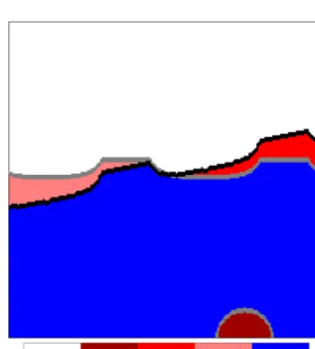
Figure 4. Depiction of areas used for computing the IIEE met-rics. The pink region corresponds to theA+area given by Eq. (9), whereas theA− area given by Eq. (10) is in red. The additional
A−area in the modified case is in dark red. Ice edges are displayed as gray lines (observations) and black lines (model results). (These lines are drawn with 3 times their actual thickness in order to accen-tuate the edges graphically.) Regions where all products are on the open ocean side of the ice edges are blue, while regions inside the ice edges in all products are white.
Now consider the areas between the ice edges, from which the IIEE metrics are computed. The regions corresponding to the definitions in Eqs. (9) and (10) are shown in pink and red in Fig. 4.
The results for the various displacement metrics that were defined in Sect. 2 are given in Table 1. First, we note that in the reference case, allDIEandDIIEEscores have similar val-ues (with the expected exception of the maximum displace-ment scoreDIEH, which has a larger value than the otherDIE
scores by design). Also,1IEand1IIEEare of similar magni-tudes in the reference case.
For the modified case, we assume that the bottom bound-ary is adjacent to land. This is relevant for the hatted ice edge displacement metrics. From experience, we know that dis-crepancies where sea ice emerges or disappears at a distance from other ice-covered regions arise from time to time in an operational sea ice forecasting service. An example will be presented in Sect. 4. We find that the values of theDIE ice edge displacement metrics given by Eqs. (4), (5), and (7) in-crease from the reference case to the modified case by a fac-tor of about 2–5 even though a fairly modest area with addi-tional sea ice has been introduced in the latter case. Since the additional discrepancy between the observations and model results has been introduced at a large distance, this change is according to our expectations.
Even though an additional discrepancy has been intro-duced in the modified case, its shape and size is such that with the exception of bias metrics all IIEE displacement met-rics increase by a very modest degree in these synthetic ex-amples. In conclusion, we find that the deterioration accord-ing to scores for the modified case is much larger for the DIEice edge displacement metrics than for the IIEE metrics since the latter do not explicitly depend on the displacement between the pair of ice edges. Moreover, we note that if the ice edge displacement is defined by Eq. (3) the resultingDdIE displacement increases only by a marginal fraction from the reference case to the modified case due to the added ice area’s proximity to land.
Table 1.Results for the various displacement metrics defined in Sect. 2. Vertical lines are introduced to separate non-negative displacement metrics from signed bias metrics and the FSS metric from IIEE metrics. The reference case and the modified case refer to the observational sea ice concentrations that are displayed in Fig. 3a and b, respectively. All values are given in non-dimensional grid units. Note that in the reference case, all boundaries are considered open, so the ice edge displacement metrics are unaffected when computing the hatted variables. Note also that in the modified case, the bottom boundary was treated as adjacent to a closed (land) boundary.
Ice edge displacement metrics
DAVGIE DIERMS DHIE D\IEAVG D\RMSIE DdIE
H 1IE 1dIE
Reference case 9.1 10.6 20 9.1 10.6 20 0.24 0.24 Modified case 17.5 27.4 112 9.2 10.7 20 −9.1 −0.8
FSS IIEE displacement metrics
DFSS DAVGIIEE D\IIEEAVG D\RMSIIEE D\IIEEMAX 1IIEE \1IIEE
Reference case 8.8 8.8 10.4 10.5 10.6 0.17 0.21 Modified case 9.8 9.6 11.0 11.1 13.4 −1.7 −2.3
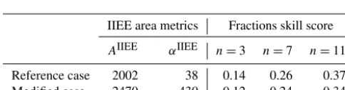
Table 2.Supplementary metric scores. IIEE area scores are given in non-dimensional grid units. The fractions skill score is computed by Eq. (21).
IIEE area metrics Fractions skill score
AIIEE αIIEE n=3 n=7 n=11 Reference case 2002 38 0.14 0.26 0.37 Modified case 2470 −430 0.12 0.24 0.34
A digression which is relevant here is that we have not included the modified Hausdorff distance, which was recom-mended by Dukhovskoy et al. (2015), in our analysis. In our formulation, this quantity is the maximum of the two terms in brackets in Eq. (5) and will generally exhibit similar results to DIEAVG but with larger magnitudes. While the sensitivity study in Dukhovskoy et al. (2015) is rich in detail, changes like contrasts between the reference case and the modified case are not considered. In their study of results from sea-sonal forecasts, Palerme et al. (2019) conclude that results for the modified Hausdorff distance are sensitive to differ-ences with similar qualitative aspects as those discussed in this section. In Sects. 4 and 5 below we will examine if dif-ferences which are qualitatively similar to the modified case have an effect on the quality assessment of the ice edge posi-tion in the forecasts from CMEMS ARC MFC.
4 Ice edge metrics for two forecasts
We compare model results with observations, which are both products that are distributed by CMEMS. The obser-vational product is the Arctic Ocean Sea Ice Concentration Chart “Svalbard” (E.U. Copernicus Marine Service Informa-tion/Norwegian Ice Service – MET Norway, 2018), which is a multi-sensor product that uses data from synthetic aperture
radar (SAR) instruments as its primary source of informa-tion (WMO, 2017). This product covers the northern Nordic Seas, the Barents Sea, and adjacent ocean regions. It is avail-able on working days as mean values on a 1 km stereographic grid and will be referred to as the ice chart data hereafter.
Model results are taken from the Arctic Ocean Physics Analysis and Forecast product. Assimilation of sea ice con-centration is implemented through the use of microwave data, while no SAR data are assimilated. The model uct will from here on be referred to as the ARC model prod-uct. In our investigation we will consider daily mean fields of sea ice concentration, which are presently distributed on a 12.5 km stereographic grid. We restrict this study to the fore-casts from the Thursday bulletins, which are available with a forecast range of 10 d (Norwegian Meteorological Institute, 2018). The microwave data that are assimilated are avail-able as the Ocean and Sea Ice Satellite Application Facility Northern Hemisphere product (Breivik et al., 2001), which is available from the CMEMS catalogue (E.U. Copernicus Ma-rine Service Information/EUMETSAT, 2018). The assimila-tion was performed 3 d prior to the Thursday bulletins. The main aim of this investigation is to provide an independent assessment of the quality of results for the ice edge and not to assess the impact of assimilation. Thus, we compare re-sults with ice chart data rather than with the microwave data. Prior to performing the analysis both products are regrid-ded. The ice chart product is aggregated onto a 13 km grid, while the ARC model product is interpolated onto the same grid (the axes of the two CMEMS products, both available on polar stereographic grids, are rotated differently). The land– sea masks of the two regridded products are overlaid so that the geographical extent of the two regridded products is iden-tical.
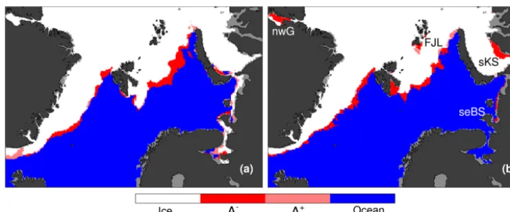
type examined in Sect. 3. The two cases that are chosen are the day 5 ARC forecast products issued on 30 March 2017 and 25 May 2017. The quality of the forecasted ice edge po-sitions will be assessed by comparing the model results with the ice edge position in the ice chart data on the respective forecast valid dates. The positions of the ice edges on these two dates according to model and observations are shown by displaying the IIEE fields in Fig. 5a and b.
For the situation on 29 May 2017 (panel b) we notice that there are large discrepancies in the position of the ice edge in several locations: a polynya to the northwest of Greenland is open in the model but not in the observations; there is a re-gion along the coast in the Barents Sea where the model ice edge has retreated from the coast in the southern Kara Sea, while the entire Kara Sea is frozen over in the ice chart; and some ice remains along the coast in the southeastern Barents Sea in the ice chart but not in the model. These objects are indicated by labels in Fig. 5. Note also that polynyas have opened around Franz Josef Land (FJL), but since these are seen in both products this region does not affect the displace-ment metrics to the same degree as the other discrepancies mentioned here.
In contrast, the situation on 3 April 2017 (panel a) has no-table offsets along the sea ice edge, but polynyas and mis-matching results in coastal regions play a much smaller role than on 29 May 2017.
Results for the various displacement metrics are given in Table 3. As was seen in the results for the synthetic cases in Sect. 3, the scores that deviate substantially between the two forecasts are for theDIEice edge displacement metrics and for1IE. The inflated values for the 29 May 2017 fore-cast compared to the results for the 3 April 2017 forefore-cast can largely be attributed to the ice edges associated with the IIEE features that are labelled in Fig. 5b. Furthermore, we note that the values forD\AVGIIEEandD\RMSIIEE are larger than those for the correspondingDdIEmetrics by a factor of 1.5–2. This contrast, which is much larger than in the synthetic case (Ta-ble 1), can be attributed to the fact that the individual IIEE features in the synthetic cases were few and regular. In the forecasts there is a large number of IIEE features with irreg-ular shapes.
Furthermore, we find that the DdIE metrics change only very modestly from 3 April 2017 to 29 May 2017 due to the proximity to the coast for the features that are labelled in Fig. 5b, in contrast to the results forDIE. We also note that the definitions for the displacement metrics that are derived from the IIEE lead to values for\DAVGIIEEthat are about twice as large as the correspondingDAVGIIEEvalues. Finally, we observe that for each of the two forecasts that are examined here, the relative difference between DAVGIIEE and\DIEAVG is only about 10 % or less. The relationships between the various displace-ment metrics are examined based on results from a full year of weekly forecast bulletins in the next section.
From the results for supplementary metrics in Table 4 we note that the FSS values are only slightly lower for the 29 May 2017 forecast than for the 3 April 2017 forecast, even though this forecast performs much poorer when diagnosed with theDIEice edge displacement metrics.
5 Ice edge position metrics for 2017
The comparison of model results and observations in Sect. 4 has been performed for all weekly forecast bulletins from 2017. The results for mean displacement metrics and biases for the 5 d forecasts are displayed in Fig. 6. We note that there is a seasonal variation in all metrics with large devia-tions during the months that lead up to the sea ice minimum in mid-September. We will refer to the period from the start of July to mid-September as the pre-minimum. A substantial part of the pre-minimum discrepancies is explained by the biases, which reveal that the sea ice extent is larger in the ice chart product than in the model product. The smaller extent in the model product gives rise to negative values in Fig. 6b. Annual average values for the various displacement metrics are given in the rows labelled “All 5 d forecasts” in Tables 3 and 4.
Furthermore, we note that the curves in Fig. 6 can be sep-arated into two groups.
1. DIEAVG,\DIIEE AVG, andD
FSS
2. \DIEAVGandDAVGIIEE
Group 1 metrics generally have larger values than group 2 metrics. This is expected since e.g.\DIE
AVG≤D IE
AVGby
defini-tion, notably the different impact on these two metrics when the displacements occur in the vicinity of land or islands. Moreover, we demonstrated in Sect. S1 that the definition of\DAVGIIEE in group 1 leads to values that are larger than the DIIEEAVGmetric in group 2.
Interestingly, we find that there is a contrast in the results between the two metrics groups during the pre-minimum: the deterioration exhibited in the evolution of group 1 metrics is larger than the corresponding deterioration for group 2 met-rics in absolute terms. When we inspect the results from the two cases presented in Sect. 4, Table 3 reveals that the group 2 metrics have the lowest values in both cases. However, the separation into two distinct groups of metrics does not ap-ply. We note that these two cases (indicated by vertical lines in Fig. 6) precede the July to mid-September pre-minimum during which the separation between the groups is most strik-ing.
Figure 5.Map displaying the IIEE regions for two forecasts. Panels(a)and(b)display the results for the forecast for 3 April 2017 issued on 30 March 2017 and for the forecast for 29 May 2017 issued on 25 May 2017, respectively. Areas displayed in gray are not included in one or both products and are excluded in the present analysis. The following regions with ice edge discrepancies are labelled in panel(b): near Franz Josef Land (FJL), southern Kara Sea (sKS), northwest of Greenland (nwG), and southeastern Barents Sea (seBS). The displayed region is nearly the same as the region with ice chart data (a slight zooming was applied in order to highlight features of interest, so narrow bands of grid cells from the ice chart data to the right and to the bottom are not shown). The colour codes for the various IIEE regions are the same as in Fig. 4.
Table 3.Results for the various sea ice edge displacement metrics. Forecast 4–3 and Forecast 5–29 results are metrics for the forecast for 3 April 2017 issued on 30 March 2017 and for the forecast for 29 May 2017 issued on 25 May 2017, respectively. All 5 d forecast results are averages for all weekly 2017 forecast bulletins with a 5 d lead time. Bootstrap fraction is the difference between the 95 percentile and 5 percentile values from a bootstrap analysis of all 5 d forecast results, divided by the corresponding average value. All values are in kilometres except the bootstrap fractions, which are non-dimensional. See the text for details.
Ice edge displacement metrics
DIEAVG DIERMS DIEH D\AVGIE D\IERMS DdIE
H 1IE 1dIE
Forecast 4–3 35 47 150 31 43 150 −14 −15 Forecast 5–29 98 230 1560 31 39 130 −87 −23 All 5 d forecasts 69 116 720 37 48 175 −55 −27 Bootstrap fraction 0.25 0.27 0.28 0.17 0.15 0.15
FSS IIEE displacement metrics
DFSS DIIEEAVG D\AVGIIEE D\IIEERMS D\MAXIIEE 1IIEE \1IIEE
Forecast 4–3 45 29 61 69 100 −14 −40 Forecast 5–29 48 34 57 61 91 −27 −48 All 5 d forecasts 61 39 79 86 119 −29 −64 Bootstrap fraction 0.28 0.18 0.18 0.18 0.15
the Supplement for details). Hence, the pre-minimum peaks that are seen in Fig. 6 can at least to some degree be attributed to the assimilation of an observational product that deviates from the ice charts during the pre-minimum season. The cor-relation coefficient for the time series of DAVGIE for the 5 d forecasts vs. ice charts (black line in Fig. 6a) and the time series ofDAVGIE for microwave data vs. ice charts is 0.89. The corresponding correlation coefficient for1IEis 0.92.
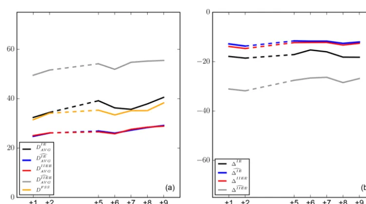
Next, we have examined how the quality of the ice edge forecasts changes as a function of lead time. In order to limit
mi-Figure 6.Time series for(a)mean displacement and(b)bias metrics as defined in Sect. 2. All results are for the 5 d forecasts. Vertical lines correspond to the two forecasts that were analysed in Sect. 4. Values along the vertical axes are in units of kilometres.
Figure 7. Metrics for(a)mean displacement and(b)bias as functions of forecast lead time in days. These results are based on forecast bulletins from January 2017 to mid-May 2017. Note that lines forD\IEAVGandDIIEEAVGin(a)nearly overlap, as do lines for1dIEand1IIEEin (b). Values along the vertical axes are in units of kilometres. Ice charts are not produced on Saturdays and Sundays, which correspond to forecast lead times of+3 and+4 d, respectively. Dashed lines are thus used to indicate the lack of analysis for these two days.
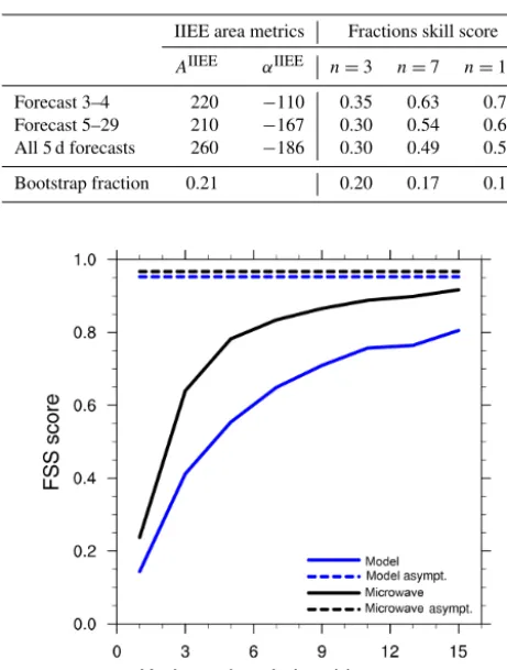
crowave data. These results reveal that useful forecasts with a 5 d lead time are obtained at a scale of about 60×60 km when the FSS reaches a value of 0.5 (which is a criterion recom-mended by Skok and Roberts, 2016). When comparing the microwave data with ice charts, the FSS is well above 0.5 for a neighbourhood extentn=3, corresponding to useful data at a scale of approximately 40×40 km if ice chart data are taken as truth.
Table 4.Supplementary metric scores for the forecasts displayed in Fig. 5 and the corresponding 2017 average values. IIEE area scores are given in units of 1000 km2.
IIEE area metrics Fractions skill score
AIIEE αIIEE n=3 n=7 n=11
Forecast 3–4 220 −110 0.35 0.63 0.75 Forecast 5–29 210 −167 0.30 0.54 0.68 All 5 d forecasts 260 −186 0.30 0.49 0.59
Bootstrap fraction 0.21 0.20 0.17 0.15
Figure 8.Fractions skill score as a function of resolution for 5 d lead time model forecasts vs. ice chart data (blue line) and mi-crowave data vs. ice chart data (black line). Dashed lines show the asymptotic FSS values as defined by Roberts and Lean (2008) (their Eq. 8). These results are based on forecast bulletins and microwave data from January 2017 to mid-May 2017.
6 Discussion
Our investigation of the results for the ice edge in the 2017 forecast bulletins in Sect. 5 revealed that the metricsD\AVGIE andDAVGIIEE nearly overlap, and this is also the case for1dIE and1IIEE. These similarities can to some degree be under-stood from the following simplified cases: consider first a sit-uation in which one ice edge is shifted by a constant distance from the other; i.e. they are parallel lines. Then, all of the av-erage displacement metrics will be nearly identical, and this will also be the case for the displacement bias metrics. This is an idealised description for cases similar to the forecast for 3 April 2017 (Fig. 5a) whereinDIEAVGis only moderately larger thanD\AVGIE (Table 3).
Next, consider a situation in which a part of one ice edge is shifted from the other, and the remaining part is due to dis-crepancies with coastal ice cover in one product but not in
the other. When the length of boundaries between IIEE ar-eas and adjacent dry grid cells is much shorter than the ice edge length, the impact of disregarding coastal segments in Eq. (13) is small. Then, nearly identical displacement met-rics values will again be the result for e.g.D\AVGIE andDAVGIIEE by the same argument as above since the coastline will have taken on the role as an ice edge or IIEE area limit. However, the value forDIEAVG will inflate in this situation. These dif-ferences in displacement metrics will be further accentuated when such coastal discrepancies are separated geographi-cally from the remaining ice edges as e.g. is seen with the labelled features in Fig. 5b, andDAVGIE D\AVGIE (Table 3).
The main exception to the two types of situations de-scribed above occurs when polynyas form in the open ocean, away from the continental coasts and the Arctic islands. However, such cases rarely arise in the set of results inves-tigated here.
Table 3 also includes results from a bootstrap analysis for the 2017 ice edge position metrics. The non-dimensional fractions that are listed are calculated by dividing the range spanned by the 5 and 95 percentile values by the mean value. Thus, smaller fractions indicate more robust results. We note that the fractions for theDIEmetrics are larger than the frac-tions for theDdIE metrics. The weakened robustness of the DIE metrics is due to the non-stationary behaviour of fea-tures that can give rise to inflated values for these metrics. Fraction values are not included for the bias metrics since bias averages can in principle be close to 0 with a combi-nation of large positive and negative values. Hence, to com-plete the bootstrap analysis we add that ranges spanned by the 5 and 95 percentile values for1dIEand1[IIEE are 9 km, while the corresponding ranges for1IEand1IIEEare 21 km. 6.1 Reducing the set of displacement metrics
The expected relationship between displacement metrics, conceptually described above, is confirmed by the results in Sect. 5. Hence, with the present configuration of validation domain and the results from the model and observations, one in each of the two metrics pairsD\AVGIE , DAVGIIEE and1dIE, 1IIEE can be disregarded. Of the two approaches, we find adopting DIIEEAVGand1IIEEto be the more intuitive and simpler choice (but admittedly this preference is somewhat subjective).
[−0.85, 0.85] are of interest, we find that 13 of the proposed 15 metrics can be divided into four groups, inside which met-rics have large positive (>0.85) or large negative (<−0.85) correlation coefficients. These groups are the following.
1. All threeDIEmetrics 2. DAVGIIEE,DFSS,D\AVGIE 3. 1dIE,1IIEE,1[IIEE
4. D\RMSIE ,\DAVGIIEE,D\IIEERMS,D\IIEEMAX
The two remaining displacement metrics are1IEandDdIE
H.
Note also that the Hausdorff maximum metrics are at times subject to large fluctuations depending on the presence or ab-sence of outliers. This was also noted in the investigation of skill metrics for sea ice model results by Dukhovskoy et al. (2015). Hence, a case can be made for disregarding the Haus-dorff maximum metrics.
6.2 Relative ice edge metrics
From the synthetic cases that were analysed in Sect. 3, we note that the penalty for local freezing in one product but not in the other is much smaller for the IIEE-based displace-ment metricDAVGIIEEthan for the ice edge displacement metric DAVGIE . We therefore introduce two combined, relative met-rics.
rAVG=
DAVGIE
DAVGIIEE (22)
d rAVG=
DAVGIE
\ DAVGIE
(23)
These derived metrics will e.g. increase in magnitude as local freezing is seen in the observational product and not in model results since the common numeratorDAVGIE will inflate. Then, if the model eventually becomes able to represent the local freezing, the metrics will decrease. For the synthetic cases we investigated in Sect. 3 we findrAVG=1.03 andrdAVG=1 in the reference case. In the modified case we haverAVG=1.82
andrdAVG=1.90. The corresponding sets of ratios for the two
forecasts that were examined in Sect. 4 arerAVG=1.21 and
d
rAVG=1.14 on 3 April 2017 andrAVG=2.89 andrdAVG= 3.17 on 29 May 2017.
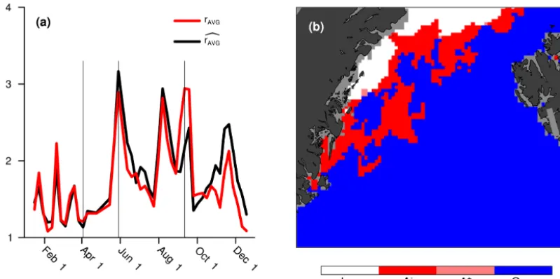
We started this discussion by noting that results for the two metrics, which are the denominators in Eqs. (22) and (23), nearly overlap. Hence, the curves in Fig. 9a also nearly overlap. However, this is not the case for the 5 d forecast for 11 September 2017, indicated by the rightmost vertical line in Fig. 9a. This outlier in the context of the metrics ra-tios can be explained by examination of the IIEE areas, for which the results in the Fram Strait are shown in Fig. 9b. We can infer that there is a complex shape of a large part of the ice edge in the observational product (the red grid cells
that have a blue neighbour), which is at some distance from the model ice edge. This inflates the edge-integrated metric \
DIEAVG much more than the area-derivedDAVGIIEE, and conse-quentlyrdAVG(2.18) is significantly smaller thanrAVG(2.94)
in this case.
6.3 Recommendation
Our recommendations regarding a set of metrics to use for assessing the quality of ice edge forecasts are made from a preference of simplicity and necessity. In terms of simplicity we have in mind metrics which are not convoluted in their implementation and also have an intuitive interpretation. In terms of necessity we have in mind a set of metrics for which each value provides useful information that is supplementary to the other values and not overlapping.
From the analysis of validation results from a full calendar year that was presented in Sect. 5 and the subsequent discus-sion in Sect. 6.1 above, we recommend that validation results for ice edge displacement be provided for a set of three met-rics.
1. DIEAVG 2. DIIEEAVG 3. 1IIEEAVG
Here, (1) and (2) give a high and a low bound for the ex-pected displacement error for the position of the ice edge, respectively. The bias metric (3) provides information about whether the ice edge should be expected before or after a user reaches the forecasted position of the ice edge.
Moreover, while no new metrics are involved, we also en-courage displaying results for
4. rAVG,
since time series for this quantity provide information on the robustness of the metrics results that can be easily presented as a line plot. In situations with large values of this fraction a user should be aware that the quality of the forecasted ice edge position is sensitive to how the displacement error is formulated. Note that of the two formulations in Eqs. (22) and (23), our preference is the former since the episodic high impact of a complex ice edge makes interpretation of the lat-ter less intuitive in the present context.
Figure 9. (a)Time series of two metrics ratios for forecasts with a lead time of 5 d. Vertical lines correspond to cases for which results are discussed in detail. The left and centre vertical lines correspond to the two forecasts that were analysed in Sect. 4, whereas the line to the right is for the situation displayed in panel(b).(b)Detail of IIEE in the Fram Strait (the region between Greenland and the Svalbard archipelago) on 11 September 2017
Obviously, in a context of forecasting, validation results will always be available after the fact only. However, recent validation results are more often than not also relevant for a future period. We apply an auto-correlation crossing at e−1 to define the decorrelation timescale. Then, we find that the decorrelation timescales of the metrics (1)–(4) above are 6– 7 weeks.
Frequently, users of forecast products are interested in the results for a small portion of the full domain. Hence, when possible validation results should be provided as easily ac-cessible representations on maps. Taking advantage of the long decorrelation timescale, we recommend supplementing the above set of metrics with maps showing the distribution of IIEE areas (e.g. Fig. 5).
This ends our recommendation for a basic set of ice edge displacement metrics. Nevertheless, more advanced users may also benefit from access to results for the FSS as a func-tion of neighbourhood size: the FSS will also be highly rel-evant when performance changes in model system upgrades due to increased resolution are evaluated.
The above set of recommendations is based on an exami-nation of results covering 1 year for a specific forecast system and a specific observational product. While we believe that such an analysis is relevant for other sets of forecasts and ob-servational products, each configuration should be checked separately if resources are available. Issues like domain size (e.g. pan-Arctic vs. regional) and resolution (representation of archipelagos and straits) can conceivably affect the char-acteristics of the forecast quality.
We end this study by noting that the travel time for com-mercial shipping between ports in northwestern Europe and the Far East is about 20–30 d with speeds in the range 10–
15 knots (5–7.5 m s−1) (Schøyen and Bråthen, 2011). Adding
a few days for advanced decision-making on sea routes, and subtracting some days for sailing time in ice-free conditions at the end of the leg, forecast lead times of up to 20–30 d are expected to be required in this context. Presently, CMEMS forecasts are available for lead times up to 10 d. We have shown that the deterioration in the forecast quality is mod-erate for these lead times (Fig. 7). Since maritime safety is one of the four core CMEMS areas of benefit, our final rec-ommendation is to double the forecast lead time range of the CMEMS forecasting systems.
The forecasts that are analysed in this investigation, however, are publicly available from http://thredds.met.no/thredds/myocean/ ARC-MFC/myoceanv2-class1-arctic.html (Norwegian Meteoro-logical Institute, 2018).
Supplement. The supplement related to this article is available online at: https://doi.org/10.5194/os-15-615-2019-supplement.
Author contributions. AM performed the analysis and wrote the ar-ticle. Based on results from the analysis, CP provided Figs. 6 and 7, with the remaining figures provided by AM. CP and MM con-tributed to discussions and provided comments and suggestions that significantly improved the presentation of the present study.
Competing interests. The authors declare that they have no conflict of interest.
Special issue statement. This article is part of the special is-sue “The Copernicus Marine Environment Monitoring Service (CMEMS): scientific advances”. It is not associated with a confer-ence.
Acknowledgements. We would like to express our gratitude to two anonymous referees whose comments and suggestions significantly improved our paper. We are also indebted to the model development team at the Nansen Environmental and Remote Sensing Center, as well as the Norwegian Ice Service at the Norwegian Meteorological Institute for the provision of the ice chart. This study was performed on behalf of the Copernicus Marine Environmental and Monitor-ing Service under Mercator Océan contract no. 2015/S 009-011301. This is a contribution to the Year of Polar Prediction (YOPP), a flag-ship activity of the Polar Prediction Project (PPP) initiated by the World Weather Research Programme (WWRP) of the World Me-teorological Organization (WMO). Figures 1–5, 8–9, S1–3, and S5 were made using the NCAR Command Language (NCL, 2017).
Financial support. This research has been supported by the Coper-nicus Programme via Mercator Océan (grant no. 2015/S 009-011301) and by the Norwegian Research Council (Nansen Legacy project (contract no. 276730) and the SALIENSEAS project (con-tract no. 276223)).
Review statement. This paper was edited by Pierre-Yves Le Traon and reviewed by two anonymous referees.
References
Arzel, O., Fichefet, T., and Goosse, H.: Sea ice evo-lution over the 20th and 21st centuries as simulated
by current AOGCMs, Ocean Model., 12, 401–415, https://doi.org/10.1016/j.ocemod.2005.08.002, 2006.
Bell, M.-J., Schiller, A, Le Traon, P.-Y., Smith, N. R., Dombrowsky, E., and Wilmer-Becker, K.: An introduc-tion to GODAE OceanView, J. Op. Oceanogr., 8, 2–11, https://doi.org/10.1080/1755876X.2015.1022041, 2015. Breivik, L.-A., Eastwood, S, Godøy, Ø, Schyberg, H,
Ander-sen, S., Tonboe, R. T.: Sea Ice Products for EUMETSAT Satel-lite Application Facility, Can. J. Remote Sens., 27, 403–410, https://doi.org/10.1080/07038992.2001.10854883, 2001. Carrieres, T., Casati, B., Caya, A., Posey, P., Metzger, E. J.,
Melsom, A., Sigmond, M., Kharin, V., and Dupont, F.: System evaluation, in: Sea Ice Analysis and Forecast-ing, edited by: Carrieres T., Buehner M., Lemieux J. F., and Pedersen, L. T., Cambridge University Press, https://doi.org/10.1017/9781108277600, 2017.
Dukhovskoy, D. S., Ubnoske, J., Blanchard-Wrigglesworth, E. , Hi-ester, H. R., and Proshutinsky, A.: Skill metrics for evaluation and comparison of sea ice models, J. Geophys. Res.-Oceans, 120, 5910–5931, https://doi.org/10.1002/2015JC010989, 2015. E.U. Copernicus Marine Service Information/EUMETSAT:
Copernicus – Marine environment monitoring service, available at: http://marine.copernicus.eu/services-portfolio/ access-to-products/?option=com_csw&view=details&product_ id=SEAICE_GLO_SEAICE_L4_NRT_OBSERVATIONS_011_ 001, last access: 12 November 2018.
E.U. Copernicus Marine Service Information/Norwegian Ice Service – MET Norway: Copernicus – Marine environment monitoring service, available at: http: //marine.copernicus.eu/services-portfolio/access-to-products/ ?option=com_csw&view=details&product_id=SEAICE_ARC_ SEAICE_L4_NRT_OBSERVATIONS_011_002, last access: 19 November 2018.
Goessling, H. F., Tietsche, S., Day, J. J., Hawkins, E., and Jung, T.: Predictability of the Arctic sea ice edge, Geophys. Res. Lett., 43, 1642–1650, https://doi.org/10.1002/2015GL067232, 2016. Goessling, H. F. and Jung, T.: A probabilistic verification
score for contours: Methodology and application to Arctic ice-edge forecast, Q. J. Roy. Meteor. Soc., 144, 735–743, https://doi.org/10.1002/qj.3242, 2018.
Hernandez, F., Bertino, L., Brassington, G., Chassignet, E., Cummings, J., Davidson, F., Drévillon, M., Garric, G., Ka-machi, M., Lellouche, J.-M., Mahdon, R, Martin, M. J., Rat-simandresy, A., and Regnier, C.: Validation and Intercom-parison Studies Within GODAE, Oceanography, 22, 128–143, https://doi.org/10.5670/oceanog.2009.71, 2009.
Ho, J.: The implications of Arctic sea ice de-cline on shipping, Mar. Policy, 34, 713–715, https://doi.org/10.1016/j.marpol.2009.10.009, 2010.
Johnson, M., Gaffigan, S., Hunke, E., and Gerdes, R.: A compari-son of Arctic Ocean sea ice concentration among the coordinated AOMIP model experiments. J. Geophys. Res., 112, C04S11, https://doi.org/10.1029/2006JC003690, 2007.
Massonnet, F., Fichefet, T., Goosse, H., Bitz, C. M., Philippon-Berthier, G., Holland, M. M., and Barriat, P.-Y.: Constraining projections of summer Arctic sea ice, The Cryosphere, 6, 1383– 1394, https://doi.org/10.5194/tc-6-1383-2012, 2012.
Melsom, A., Simonsen, M., and Bertino L.: MyOcean Project Scientific Validation Report (ScVR) for V1 real-time forecasts, Tech. Rep., met. no, Oslo, Norway, 21 pp., available at: http: //cmems.met.no/ARC-MFC/Validation/validationReport01.pdf (last access: 4 December 2018), 2011.
The NCAR Command Language (Version 6.4.0) [Soft-ware], Boulder, Colorado: UCAR/NCAR/CISL/TDD, https://doi.org/10.5065/D6WD3XH5, 2017.
Norwegian Meteorological Institute: TOPAZ4 Ocean Physical Fields, available at: http://thredds.met.no/thredds/myocean/ ARC-MFC/myoceanv2-class1-arctic.html, last access: 16 November 2018.
Palerme, C., Müller, M., and Melsom, A.: An intercompari-son of skill scores for evaluating the sea ice edge position in seasonal forecasts, Geophys. Res. Lett., 46, 4757–4763, https://doi.org/10.1029/2019GL082482, 2019.
Posey, P. G., Metzger, E. J., Wallcraft, A. J., Hebert, D. A., Al-lard, R. A., Smedstad, O. M., Phelps, M. W., Fetterer, F., Stew-art, J. S., Meier, W. N., and Helfrich, S. R.: Improving Arctic sea ice edge forecasts by assimilating high horizontal resolution sea ice concentration data into the US Navy’s ice forecast sys-tems, The Cryosphere, 9, 1735–1745, https://doi.org/10.5194/tc-9-1735-2015, 2015.
Roberts, N. M. and Lean, H. W.: Scale-Selective Verifica-tion of Rainfall AccumulaVerifica-tions from High-ResoluVerifica-tion Fore-casts of Convective Events, Mon. Weather Rev., 136, 78–97, https://doi.org/10.1175/2007MWR2123.1, 2008.
Schøyen, H. and Bråthen, S.: The Northern Sea Route versus the Suez Canal: cases from bulk shipping, J. Transp. Geogr., 19, 977–983, https://doi.org/10.1016/j.jtrangeo.2011.03.003, 2011. Skok, G. and Roberts, N. M.: Analysis of Fractions Skill Score
properties for random precipitation fields and ECMWF forecasts, Q. J. Roy. Meteor. Soc., 142, 2599–2610, https://doi.org/10.1002/qj.2849, 2016.
Skok, G. and Roberts, N. M.: Estimating the displacement in precip-itation forecasts using the Fractions Skill Score, Q. J. Roy. Me-teor. Soc., 144, 414–425, https://doi.org/10.1002/qj.3212, 2018. WMO: Sea-Ice Information Services in the World, WMO No. 574,
World Meteorological Organization, 103 pp., 2017.