ENERGY MANAGEMENT OF
WIRELESS SENSOR NETWORK WITH
MIMO TECHNIQUES
TRUPTI MAYEE BEHERA
School of Electronics, KIIT University Bhubaneswar, Odisha,India [email protected] SUDHANSU SEKHAR SINGH
School of Electronics, KIIT University, Bhubaneswar, Odisha,India
Abstract :
With recent advances in deployment of sensor nodes mounted on mobile platforms, node mobility is becoming an attractive alternative to improve network coverage dynamically in sensor networks. Mobile sensor networks deployed for surveillance applications, it is important to use an efficient energy management scheme that can empower nodes to make better decisions regarding their positions such that strategic tasks like target tracking can be benefited from node movement. However, due to energy constrain nodes; it may not be cost effective to deploy a large number of mobile nodes for continuous movements. Due to their effectiveness for enhancing energy and bandwidth efficiency, MIMO schemes have been studied intensively in recent years and used for energy conservation.
Keywords
—
Wireless sensor networks, Energy efficiency, Virtual MIMO, STBC, SCHCT
1. Introduction
Energy consumption is the core issue in wireless sensor networks (WSN). To generate a node energy model that can accurately reveal the energy consumption of sensor nodes is an extremely important part of protocol development, system design and performance evaluation in WSNs[1]. Due to the physical size and energy limitation of small sensor nodes, directly deployment of MIMO in one sensor node is infeasible in practice. However, through sensor nodes cooperation, virtual MIMO technique can be implemented in sensor networks. In virtual MIMO network, a group of sensors cooperate to transmit and receive data. Space–time block coding [2][3] is a technique used in wireless communications to transmit multiple copies of a data stream across a number of antennas and to exploit the various received versions of the data to improve the reliability of data-transfer. Hence in this paper the STBC based cluster heads cooperative transmission (SCHCT) scheme is proposed.
2. System Model
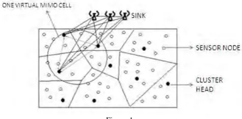
Figure 1
The sink is assumed to be equipped with more than one antenna in order to implement the MIMO transmission. Each node has a packet of L bits to the cluster head. The operation of SCHCT is divided into rounds [4]. Each round consists of three stages: the cluster formation stage, the steady state stage and the cooperative transmission stage
2.1. Cluster Formation Stage
Step 1: In this stage, all the sensor nodes self-organized to form clusters. Each node in the network uses the classic carrier sense multiple access with collision avoidance (CSMA/CA) scheme to contend for the wireless channel [5]. Once a node ‘x’ succeeds in accessing the channel, it sends a message at fixed transmission energy to discover its one-hop neighbours. This message carries the following information: node ID, its remaining energy, and a list of x's neighbours (nodes that x has received messages from). In general, a node sends messages as soon as it joins the network and whenever it hears from new neighbours.
Step 2: The next step is to select the Master cluster head (MCH). Since MCHs do more work than any typical node (for collecting, aggregating, and forwarding data), the selection criterion of MCHs is the node's remaining energy. Each node maintains tables of remaining energy values of all its 1-hop neighbours’ .All the nodes start the clustering process .Every node compares its remaining energy to those of its one-hop neighbours. A node waits for other undecided neighbours with higher remaining energy to decide before itself. If the node has the highest remaining energy in its neighbourhood, it declares itself as an MCH and announces that to its neighbours.
Step 3: The next step is to associate a Slave cluster head (SCH) with each MCH, if possible. To select SCHs, each MCH sends an SCH invitation message to the neighbouring node whose neighbour list overlaps the most with that MCH's neighbour list. The invited node announces its decision via an SCH acceptance message, enabling decided MCHs to look for other SCHs. Upon receiving an SCH acceptance message, the intended MCH confirms this association via an SCH confirmation message.
Step 4: After the election of the cluster heads, each cluster head will transmit a broadcast message to other sensor nodes in the area using CSMA protocol. The message contains the cluster head’s ID. Sensor nodes then choose one of the cluster head to join in based on the signal strength of the broadcast message. By sending the join-request message to the nearest cluster head, the cluster head will record the ID of the cluster members. After the formation of the cluster, the cluster head will set up a TDMA schedule for the cluster members and then broadcast this schedule to each of the cluster members.
2.2 Steady State Stage
In this phase, cluster members will transmit their data to the cluster head by multiple frames as in the original LEACH scheme. In each frame, each cluster member will transmit its data during its allocated transmission slot specified by the TDMA schedule in cluster formation phase, and it will be sleep in other slots to save energy. After a cluster head receives data frames from its cluster members, it will perform data aggregation to remove the redundancy in the data.
2.3 Cooperative Transmission Stage
3 WORK APPROACH
In the analysis, the following assumptions are made:
i) There are N nodes distributed uniformly in an M × M region
ii) An AWGN (Additive White Gaussian Noise) channel with squared path loss is assumed for the intra-cluster communication,
iii) A flat Rayleigh fading channel with a power loss is assumed for the inter cluster communication iv) BPSK is used as modulation scheme.
3.1 Communication Energy Consumption Model
In order to model the energy consumption of the whole network, the energy consumption of transmitting or receiving one bit is modelled firstly[8]. The total average power consumption along the signal path can be divided into two main components: the power consumption of all the power amplifiers PPA and the power
consumption of all other circuit blocks Pc. The first term PPA is dependent on the transmit power Pout, which can
be calculated according .The transmitting energy consumption of one bit is defined as: Ebt = (PPA + PC) / Rb
Where Ebt is the energy consumption of transmitting one bit when both circuitry and transmission energy
consumption are considered, PPA is the power consumption of all power amplifiers, PC is the power consumption
of all other circuit blocks and Rb is the bit rate of the system.
The power consumption of the power amplifiers can be approximated as : PPA = (1+ α) Pout
Where α is the efficiency of radio frequency power amplifier. Thus Pout can be estimated as:
>
≤
Π
=
o r t t r f l b b r t f l b b outd
d
d
h
h
G
G
N
M
R
E
d
d
d
G
G
N
M
R
E
P
;
;
)
4
(
4 2 2 0 2 2 2λ
Where Eb is the required average energy per bit at the receiver for a given BER requirement Pb, Rb is the system
bit rate, d is the transmission distance, d0 is the distance threshold and defined as 4πhthr/λ. Gt is the transmitter
antenna gain, Gr is the receiver antenna gain, λ is the carrier wavelength, ht and hr are the heights of transmitter
and receiver antenna, Ml is the link margin compensating the hardware process variations and other additive
background noise or interference. Nf is the receiver noise figure defined as Nf = Nr/N0, where N0 is the
single-sided thermal noise power spectral density (PSD) at room temperature, and Nr is the PSD of the total effective
noise at the receiver input.
Denote by Pct and Pcr the power consumption of transmitting circuit blocks and receiving circuit blocks,
respectively. As in [11], Pct can be estimated as:
Pct≈ PDAC + Pmix + Pfilt + Psyn
And Pcrcan be estimated as:
P
cr≈
P
LNA+ P
syn+ P
mix+P
IFA+ P
filr+ P
ADCwhere PDAC, Pmix, Pfilt, Psyn, PLNA, PIFA, Pfilr, PADC are the power consumption for D/A converter, the mixer, the
filters at the transmitter side, the frequency synthesizer, the low noise amplifier, the intermediate frequency amplifier, the active filters at the receiver side and the A/D converter, respectively.
The total power consumption in all the circuit blocks during the long-haul communications step consists of power consumption in NT number of transmitter circuits and NR number of receiver circuits:
PC =NT (PDAC+Pmix+Pfilt+Psyn) + NR (PLNA+Psyn+Pmix+PIFA+Pfilr+PADC)
I.
Long haul transmission:
consumption of transmitting one bit for long haul MIMO transmission from cluster head to sink can be calculated as:
E
bt_MIMO= (1+
α
) E
b_MIMOb ct T toS t r t r f l
R
P
N
d
h
h
G
G
N
M
+
4 2 2where dtoS is the distance from the cluster head to the sink, Rbis the bit rate of the system, which is assumed to be equal to Bb, and B is the transmission bandwidth. Eb_MIMOis the required average energy per bit for a given BER
II. Intra-cluster transmission:
In this phase, the non-cluster head nodes send their data frames to the cluster head during their allocated time slot. The duration and the number of frames are same for all clusters and depend on the number of non-cluster head nodes in the cluster. The energy consumption of transmitting one bit from one cluster member to cluster head in one virtual MIMO cell can be calculated as:
Ebt_intra = (1+α) Eb_intra
Bb
P
d
G
G
N
M
ct CtoCH r t f l+
Π
2 2 2)
4
(
λ
Where Eb_intra is the required energy per bit for a given BER requirement, dtoCHis the distance from the cluster member to cluster head in one virtual MIMO cell.
III. Inter-cluster transmission:
After a cluster head receives data frames from its cluster members, it performs data aggregation and broadcasts the data to virtual MIMO sending nodes. When each cooperative sending node receives the data packet, they encode the data using space time block code (STBC) and transmit the data cooperatively. The energy consumption of transmitting one bit from cluster head to cluster head in one virtual MIMO cell can be calculated as:
Ebt_inter = (1+α) Eb_inter
Bb
P
d
G
G
N
M
ct CtoC r t f l+
Π
2 2 2)
4
(
λ
where Eb_interis the required energy per bit for a given BER requirement, dCtoCis the distance from the cluster head to cluster head in one virtual MIMO cell.
A. Total Energy Consumption Model of the Proposed Scheme
Energy consumption of the proposed SCHCT scheme consists of two terms: energy consumption for the cluster heads and energy consumption for the sensor nodes.[9]
1) Energy Consumption for cluster heads:
If there are Kc clusters, then there are average N/Kc nodes per cluster. Then the total energy required in one
cluster, Ecluster is given by:
Ecluster = (N/Kc-1) Es +ECH
Where Es is the energy consumption for a cluster member and ECH is the energy consumption for a cluster
head.
For each cluster head, the energy consumption consists of receiving data from the cluster members, aggregating the received data, transmitting the aggregated data to the cooperative cluster heads, receiving aggregated data from other cooperative cluster heads in the virtual MIMO cell, transmitting the encoded data to the sink by virtual MIMO technique. Therefore, the energy consumption for the cluster head is given by:
ECH=L(N/Kc-1)Ebr+L(N/Kc)EDA+L(NT-1)Ebr+LEbt_inter +LEbt_MIMO
where E
DAis the aggregation energy consumption per bit.
2) Energy Consumption by sensor nodes:
For sensor nodes in clusters, the action is only transmission of data to the cluster head, so the energy consumption is given by:
Es=LEbt_intra
Ebr= Pcr / (Bb)
Based on the above analysis, the overall energy consumption in one round of the SCHCT scheme can be derived as:
Etotal = Kc Ecluster
= (N-Kc) Es + KcECH
The above equation gives the total energy consumption in an M×M MIMO network. By approximating the bound asequality [10], we can calculate the total energy consumption per bit for the MISO system as: EMISO = (1+α) [ NtNo / Pb1/Mt ] ×[ (4πd)2 /GtGrλ2] × [MlNf] + (Pc/Rb)
4 Simulation and results
The analysis of the proposed cooperative multihop MIMO scheme is carried out using MATLAB to evaluate the energy consumption and maximize the lifetime of the sensor network.
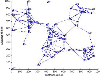
Deploying the sensor nodes
50 static wireless sensor nodes will be randomly deployed in a 1000 x 1000 area; the
communication range of each sensor node is 200 meters and the distance measurement range
is assumed as the same as the communication range. All sensor nodes have radio module for
communication and are equipped with an ultrasound transceiver for the distance measurement. It is also
assumed that each node has at least three one-hop neighbours. This is done to get unique realization for the network scenario. According to the design scheme the sensor nodes are randomly deployed in the given space then connecting each two nodes if the distance between them less than or equal to the communication radius which is shown by the Figure-1.Figurewise description for 2,3,4,5,6,7.0 100 200 300 400 500 600 700 800 900 1000 0 100 200 300 400 500 600 700 800 900 1000 1
Distance d in m
D ista n ce d i n m 2 3 4 5 6 7 8 9 10 11 12 13 14 15 16 17 18 19 20 21 22 23 24 25 26 27 28 29 30 31 32 33 34 35 36 37 38 39 40 41 42 43 44 45 46 47 48 49 50
Figure 1(Deployment of Sensor)
Energy Consumption at different stages:
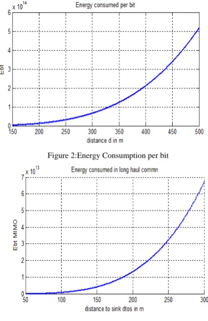
A sensing field of dimension M×M (M =200 m) with a population of N= 400 nodes is considered for simulation. Other system parameters are fc=2.5GHz, B=10kHz, α=0.4706, Ml=40dB, Nf=10dB, GtGr=5dB, ht=hr=1m,
Figure 2:Energy Consumption per bit
Figure 3:Energy Consumption in long-haul communication
Figure 5:MISO v/s MIMO (4X4)
Figure 6: Total Energy Consumption over distance dtos
0 200 400 600 800 1000 1200
0 10 20 30 40 50 60 70 80 90 100
Time(round)
P
e
rc
e
nt
ag
e of
no
de
s
al
iv
e
SCHCT ,Nt=8 SCHCT,NT=4 LEACH
5 Conclusions
Based on the basic mobile energy consumption model, the overall energy consumption model of the proposed scheme is derived which shows that although the energy consumption in MISO is less in comparison to other traditional techniques but when distance from sink increases MIMO outperforms MISO.A cluster-based cooperative MIMO scheme for multihop WSN has been explored to minimize the energy consumption and increase the lifetime of sensor nodes and the performance of the system is evaluated. The energy consumption is less when the number of transmitting antenna is minimized. When compared with LEACH scheme, numerical and simulation results together show that the proposed scheme can prolong the sensor network lifetime greatly when the distance to sink is above a threshold, especially in situations where the sink is far from the sensor area.
REFERENCES
[1] V. Tarokh, H. Jafarkhani and A. Calderbank, “Space- Time Block Codes from orthogonal Design,” IEEE Trans. Inform. Theory, vol 45, no.5, pp. 1456-1466, July 1999.
[2] S. Cui, A. J. Goldsmith and A. Bahai, “Energy efficiency of MIMO and Cooperative MIMO Techniques in Sensor Networks,” IEEE Journal of Selected Areas in Communications, vol.22, pp.1089-1098, Aug. 2004
[3] Yong Yuan, Min Chen and Taekyoung Kwon, “A novel cluster-based cooperative MIMO scheme for multi-hop wireless sensor networks,” EURASIP Journal on Wireless Communications and Networking, vol. 2006, pp. 1-9, 2006.
[4] Y. Yuan, Z. He and M. Chen, “Virtual MIMO- based cross-layer design for wireless sensor networks”, IEEE Transactions on Vehicular Technology, vol. 55, no.3, pp. 856 -864, 2006
[5] X. Li, M. Chen and W. Liu, "Application of STBC encoded cooperative transmissions in wireless sensor networks", IEEE Signal V. Tarokh, H. Jafarkham, A. R. Calderbank, “Space-Time Block Coding for Wireless
[6] Communications: Performance Results”, IEEE Journal on Selected Areas in Communications. Vol. 17, No. 3, pp. 451-460, March 1999Processing Letters, Vol.22, No. 2, pp. 134-1 37, February 2005.
[7] S. Bandyopadhyay and E. J. Coyle, “An energy efficient hierarchical clustering algorithm for wireless sensor networks,” in Proceedings of INFOCOM 2003, April 2003.
[8] ‘Cross layer optimization in energy constrained networks‘ by Aung Aung and Shuguang Cui, Stanford University
[9] Yong Yuan, Min Chen and Taekyoung Kwon, ―A novel cluster-based cooperative MIMO scheme for multi-hop wireless sensor networks, EURASIP Journal on Wireless Communications and Networking, vol. 2006, pp. 1-9, 2006.