www.nat-hazards-earth-syst-sci.net/11/2821/2011/ doi:10.5194/nhess-11-2821-2011
© Author(s) 2011. CC Attribution 3.0 License.
and Earth
System Sciences
High-resolution refinement of a storm loss model and estimation of
return periods of loss-intensive storms over Germany
M. G. Donat1,3, T. Pardowitz1, G. C. Leckebusch1,4, U. Ulbrich1, and O. Burghoff2
1Institute of Meteorology, Freie Universit¨at Berlin, Berlin, Germany
2Gesamtverband der Deutschen Versicherungswirtschaft e.V., German Insurance Association, Berlin, Germany 3Climate Change Research Centre, University of New South Wales, Sydney, Australia
4School of Geography, Earth and Environmental Sciences, University of Birmingham, Birmingham, UK
Received: 13 January 2011 – Revised: 10 September 2011 – Accepted: 18 September 2011 – Published: 25 October 2011
Abstract. A refined model for the calculation of storm losses is presented, making use of high-resolution insurance loss records for Germany and allowing loss estimates on a spatial level of administrative districts and for single storm events. Storm losses are calculated on the basis of wind speeds from both ERA-Interim and NCEP reanalyses. The loss model reproduces the spatial distribution of observed losses well by taking specific regional loss characteristics into account. This also permits high-accuracy estimates of total cumulated losses, though slightly underestimating the country-wide loss sums for storm “Kyrill”, the most severe event in the insur-ance loss records from 1997 to 2007. A larger deviation, which is assigned to the relatively coarse resolution of the NCEP reanalysis, is only found for one specific rather small-scale event, not adequately captured by this dataset.
The loss model is subsequently applied to the complete re-analysis period to extend the storm event catalogue to cover years when no systematic insurance records are available. This allows the consideration of loss-intensive storm events back to 1948, enlarging the event catalogue to cover the re-cent 60+ years, and to investigate the statistical characteris-tics of severe storm loss events in Germany based on a larger sample than provided by the insurance records only. Extreme value analysis is applied to the loss data to estimate the re-turn periods of loss-intensive storms, yielding a rere-turn pe-riod for storm “Kyrill”, for example, of approximately 15 to 21 years.
Correspondence to: M. G. Donat ([email protected])
1 Introduction
Winter storms are one of the major natural hazards in Eu-rope, often entailing substantial damage, the risk of injury or even loss of lives. Affecting relatively large areas compared to other hazards, these events cause high loss amounts, of-ten aggregating to several billion C. For example, the recent storm “Kyrill” in January 2007 (storm names used in this study as assigned by the German Weather Service, DWD) caused insured losses exceeding four billion C, even greater total economic losses, at least 46 fatalities and uprooted more than 60 million trees in Central Europe (Fink et al., 2009). Average annual wind-storm-related insured costs in Germany to residential buildings alone add up to about 900 million C (GDV, 2006, 2009). High losses also occur to pub-lic, private and economic sectors, but the most reliable and systematic records are those collected by insurance compa-nies. For statistical purposes, the German Insurance Associa-tion (Gesamtverband der Deutschen Versicherungswirtschaft e.V., GDV) compiles loss data from most insurance compa-nies present on the German market. In Germany, almost all the private sector is insured, and the insurance density of resi-dential buildings is about 85 %. It can, therefore, be assumed that the GDV loss records provide a representative picture of storm losses in this region.
2822 M. G. Donat et al.: High-resolution refinement of a storm loss model relevantly, the wind power (∼v3), i.e., the rate at which work
is performed by the kinetic energy of the wind. Other ap-proaches derive local empirical relations between vulnera-bility and wind speed and calculate the losses as a function of hazard (i.e., wind speed related to probability), vulnera-bility and the spatial distribution of values (e.g., Heneka et al., 2006; Schwierz et al., 2010). A probabilistic approach for the calculation of storm losses was recently suggested by Heneka and Hofherr (2011).
The statistical characteristic of extreme wind speeds and storms under recent climate conditions (in terms of assign-ing return periods to historic extreme storm events) was in-vestigated by a small number of previous studies. Hofherr and Kunz (2010) and Kunz et al. (2010), for example, anal-ysed extreme local wind speeds for different return periods in Germany using high-resolution wind datasets derived from regional climate models and a high-resolution limited-area model. To assess the occurrence of severe storms from a more integrated perspective, Della-Marta et al. (2009) calcu-lated continental-scale extreme wind indices for Europe and estimated the return periods of storm events during the sec-ond half of the 20th century. Brodin and Rootzen (2009) investigated extreme wind storm losses using data provided by the largest Swedish insurance company.
For this study, loss data in a high temporal and spatial reso-lution (i.e., daily loss records for 439 administrative districts in Germany) were made available by GDV for the first time for scientific purposes. These data permit the definition of the loss model at a high spatial resolution, and on the basis of individual events rather than annual loss sums. Taking into account specific regional characteristics regarding wind-loss relations, such a refinement allows accurate calculations of both the spatial loss distribution and cumulated losses for se-vere storm events. In a further step, the refined loss model is used to extend the loss data catalogue backwards, for years when losses were not yet systematically recorded by insur-ance companies. This is done by applying the loss model to NCEP reanalysis, enabling us to identify loss-intensive storms back to 1948. The extended storm catalogue finally permits a more precise estimation of the return periods of se-vere winter storms in Germany. The two main objectives of this paper are to investigate the wind-loss relation on a re-gional scale and to quantify the risk of extreme storm losses in Germany.
A description of the data and methods used is presented in Sect. 2 of this paper, followed by an explanation of the storm loss model in Sect. 3, including its verification for a number of storm events. Section 4 investigates the return periods of severe and loss-intensive winter storm events on the basis of both insurance loss records and calculated losses. The study concludes with a summary and discussion of the results in Sect. 5.
2 Data and methods
This section summarises the data and methods used for the work presented in this article. The development of the storm loss model is, however, a central point of this study and its concept will be described separately in Sect. 3.
2.1 Insurance loss data
For this study, the GDV provided loss records on a daily ba-sis, for each of the 439 administrative districts (Landkreise) of Germany. This number reflects the status in 2006; subse-quent (political) district reforms have been ignored for rea-sons of homogeneity. The administrative districts comprise of areas between 250 and 3000 km2. The loss data con-tain information on damage to residential buildings (“com-prehensive insurance on buildings”, in German Verbun-dene Wohngeb¨aude Versicherung, hereafter VGV) caused by storm or hail. It may be assumed that losses during the win-ter season are exclusively caused by extra-tropical storms, whereas convective events (including hail) play a major role during summer. For the purpose of this study, we, there-fore, restricted our analyses to the winter half year (October to March). We further checked whether the identified loss events were indeed related to a synoptic-scale winter storm by reviewing historic weather records. On the spatial scale of administrative districts, daily VGV loss data are available for the years 1997 to 2007. These data were used to derive the regional relations between wind speeds and losses (compare Sect. 3.1).
For investigating local wind-loss relations, only those storm events generating significant losses were considered. Major loss events were identified from loss frequencies (i.e., number of claimed losses relative to the total number of in-surance contracts) if the loss frequency on a specific day (or a sequence of up to three consecutive days) exceeded the loss frequency of an average day by factor 7. In Germany, this is equivalent to a loss frequency larger than 1.5 ‰. Note that this stationary criterion does not account for changes in the vulnerability of buildings with time. On the basis of this cri-terion, 34 major loss events were identified in the 11-year pe-riod from 1997 to 2007 (Table 1). They were all associated with meteorological storm situations and were used to cali-brate local wind-loss relations (Sect. 3.1). The loss amounts were calculated in loss ratios, i.e., the ratio between insured claims and totally insured values (unit: C per 1000 C i.e., in ‰). An advantage of this measure is that inflation can be neglected as it is included both in insured values and in the loss.
the insurance loss catalogue to enlarge the data basis for our investigations. Vehicle damage caused by natural hazards showed high correlations with the VGV data for the over-lapping period 1997–2007; particularly for days with signif-icant losses and when summer and winter seasons were dis-tinguished. This close relation was used to derive daily loss ratio estimates for the 1984–2008 period. A linear regression between country-wide losses to vehicles (loss needs, i.e., ra-tio between claims expenditure in C and annual units; one annual unit represents one vehicle which was insured for a complete year) and to residential buildings (loss ratio) is cal-culated based on daily country-wide losses (Fig. 1), with a coefficient of determinationR2 reaching 0.88. This regres-sion was found to be optimal for the extended winter season from October to April. These loss estimates to residential buildings simulated from the vehicle physical damage insur-ance data are hereafter referred to as VGV Sim. They are used for validation purposes and for extending the loss data catalogue and permit loss estimates in good agreement with VGV.
2.2 Meteorological data
Wind fields from two different reanalysis datasets are used to derive the local relationships between wind speed and loss and to calculate storm losses for historical events. Both ERA-Interim (Dee et al., 2011) and NCEP (Kalnay et al., 1996) reanalyses cover the whole period 1997–2007 for which VGV data are available to calibrate the loss functions (see Sect. 3.1). These relations can then be applied to the com-plete datasets and allow the calculation of storm losses back to 1948 (NCEP) and 1989 (ERA-Interim).
The atmospheric model employed to produce the ERA-Interim reanalysis uses a T255 spherical-harmonic represen-tation for the basic dynamical fields, on 60 vertical levels up to 0.1 hPa. The surface fields are provided on a reduced Gaussian grid with approximately uniform 79 km (0.7◦) spacing. The model behind the NCEP reanalysis is consid-erably coarser in resolution; it works on a T62 spectral grid with 17 vertical levels up to 10 hPa. The NCEP data are pro-vided on a 2.5◦×2.5◦grid (approximately 180 km×275 km over Germany).
Daily maximum near-surface wind speeds are used for the loss calculations. ERA-Interim provides the wind speed in 10 m height as a model output, and from NCEP we use the wind speed on the lowest model layer. The near-surface wind speeds are available as six-hourly instantaneous values, i.e., four values per day. The daily maximum is calculated as the maximum of these four values (and is hereafter referred to as wimax). Additionally, a maximum gust wind speed of all model integration time steps is available for ERA-Interim. As the physical processes related to wind gusts are generally not resolved by atmospheric models on the scale considered, gusts are calculated as a model diagnostic. The gust param-eterisation implemented in ERA-Interim takes into account
Table 1. Major loss events in the period 1997–2007 identified from the VGV data are used for the calibration of the loss model. Events are identified on the basis of loss frequencies (i.e., number of claimed losses relative to the total number of insurance contracts) exceeding 1.5 ‰.
Loss Ratio
Name Start Date End Date VGV [‰]
Ariane 19970212 19970214 0.005
Daniela 19970218 19970221 0.013
Heidi 19970224 19970226 0.007
Sonja 19970326 19970329 0.015
Fanny 19980103 19980106 0.011
Elvira-Farah 19980303 19980306 0.017
Xylia-Winnie 19981023 19981029 0.020
Maren 19981212 19981214 0.003
Lara 19990204 19990206 0.008
Anatol 19991202 19991205 0.027
Lothar 19991224 19991227 0.110
Kerstin 20000128 20000131 0.007
Oratia 20001029 20001031 0.007
Ilse 20001212 20001214 0.003
Noah 20011227 20011229 0.005
Jennifer 20020125 20020130 0.028
Natascha 20020203 20020205 0.004
Wisia 20020218 20020220 0.003
Zarah 20020221 20020224 0.004
Anna 20020225 20020301 0.031
Herta 20020308 20020310 0.004
Jeanett 20021026 20021029 0.102
Calvann 20030101 20030103 0.008
Gerda-Hanna 20040111 20040113 0.006
Queenie 20040130 20040202 0.013
Ursula 20040206 20040209 0.004
Oralie 20040319 20040322 0.019
Pia-Quimburga 20041116 20041120 0.003
Erwin 20050107 20050109 0.010
Ingo 20050119 20050121 0.005
Ulf 20050211 20050213 0.009
Dorian 20051215 20051217 0.016
Britta 20061031 20061102 0.003
Kyrill 20070117 20070119 0.242
2824 M. G. Donat et al.: High-resolution refinement of a storm loss model
21
Figures and Tables
1
2
3
Figure 1: Regression of loss needs in motor vehicle insurance and losses to residential 4
buildings caused by natural hazards during the extended winter season October-April 5
(y=0.040 * x). The dots represent country-wide daily loss values. 6
7
Fig. 1. Regression of loss needs in motor vehicle insurance and
losses to residential buildings caused by natural hazards during the extended winter season October–April (y = 0.040·x). The dots rep-resent country-wide daily loss values.
simulated wind speeds (Della-Marta et al., 2009). However, Kiss et al. (2009) found ERA-Interim-based wind power esti-mates adequate in comparison with observations, particularly when scaling the reanalysis wind speeds towards the mea-surements. The use of mesoscale models, accounting for lo-cal orographic characteristics, provides high-resolution wind fields with a considerably higher spatial variability and yields good agreement with wind speed observations (Hofherr and Kunz, 2010). However, the approach used in this study to calculate storm losses normalises wind speeds relative to the local wind climatology and, thus, leads to considerably smoothed hazard fields, also when applied to regional cli-mate model wind speeds (compare Donat et al., 2010a). Nev-ertheless, the use of high-resolution wind fields may be ben-eficial for calculating storm losses.
2.3 Identifying loss-intensive wind storm events from daily loss data
The refined loss model and also the daily VGV Sim insur-ance data are used to extend the loss data catalogue in this study. For this purpose, daily loss sums for Germany are calculated on the basis of both VGV Sim insurance records and by applying the refined loss model to the reanalysis data. To consider losses from storm events (which may affect Ger-many for more than one day), we calculated five-day running sums of losses. Further, a declustering criterion is applied to ensure that only independent storm events are considered for the calculation of return periods of the storm events. To this end, the individual storm events must occur within non-overlapping five-day periods which are separated by at least one day. This time interval appears reasonable to account
for typical travelling velocities of extra-tropical storms (or-der of magnitude≈103km per day), but also for sequences of storms which may hit Germany within a few days. We subsequently checked the meteorological conditions during the identified storm episodes to establish whether the occur-rence of storm losses were reasonable. This was done by examining the weather records in the Berliner Wetterkarte (since 1950; Berliner Wetterkarte, 2009) and Potsdamer Wet-terkarte (before 1950; Potsdamer WetWet-terkarte, 1949).
The most significant losses related to a storm generally occur only during one or two days; hence the calculated losses for the individual storm events are mostly similar if, for example, three-day running sums are considered instead of five-day sums. Some sensitivity is found only for “Vivian” and “Wiebke”, which caused heavy damage within only five days in February 1990. In the case of five-day sums, the two storms are considered as one loss event, but shorter time intervals would mean that the two loss events would not be captured properly, as the declustering criterion would lead to the exclusion of one of the two events. Therefore, calculat-ing five-day runncalculat-ing sums seems to be a good compromise in terms of capturing all major loss events contained in the data. However, it means that sequenced storm events occur-ring within a five-day period are considered as one loss event. 2.4 Extreme value analysis
To estimate the statistical characteristics of the extreme storm losses, we fit a Generalised Pareto Distribution (GPD, Coles 2001) to the loss data of the different events. In recent studies the GPD was, for example, applied to model local extreme wind speeds (Kunz et al., 2010) and also cumulated indices for storm severity (Della-Marta et al., 2009). Like them, we use the Peaks Over Threshold (POT) approach, considering all loss ratios exceeding a specific threshold for fitting the GPD. A GPD distributed variable zhas a cumulative dis-tribution function H that is characterised by threshold (u), shape parameter (ξ) and the scale parameter (σ):
H (z,u,σ,ξ )=1−
1+ξ(z−u)
σ
−1/ξ
(1) The parameters ξ andσ are estimated following the Max-imum Likelihood principle. For calculation of the N-year return level, Eq. (1) can be rewritten as
zN=u+ σ ξ
(λN )ξ−1
(2) whereλis the mean number of threshold exceedences per year.
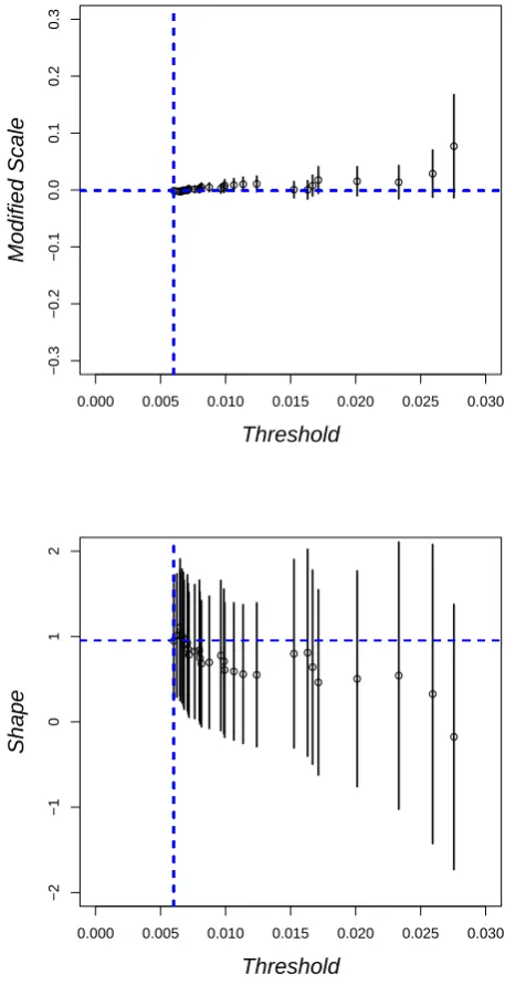
thresholds. The GPD fit is calculated for all possible thresh-olds in the samples by scanning through the ordered sam-ple of loss values and decreasing the number of considered events one by one. For all of these possible thresholds, the scale and shape parameters are estimated (see Fig. 2 for an example). Generally, higher thresholds lead to larger confi-dence intervals (estimated using the analytical Delta method) of the parameter estimates. As the result of the optimisation process, we consider the lowest possible value for which the 95 % confidence interval forξ andσ still overlaps with the confidence intervals for all higher thresholds.
3 High-resolution refinement of the loss model 3.1 Concept of the loss model
The loss model refined and applied in this study is based on the assumptions that storm losses occur locally for wind speeds exceeding the local 98th percentile of daily maximum wind speeds and grow according to a cubic function between wind and loss. Such an approach was successfully applied in a number of previous studies, proving its applicability for the calculation of storm losses in a (spatially and temporally) cu-mulated perspective (Klawa and Ulbrich, 2003; Leckebusch et al., 2007; Pinto et al., 2007; Donat et al., 2010a, 2011a). In these studies, a linear regression was used to scale country-wide annual loss potentials to the insurance loss ratios.
In this study, the availability of high-resolution insurance loss data (see Sect. 2.1) allows a refinement of the loss cal-culations. This refinement is based on the assumption that the coefficients defining the relation between wind and loss may differ regionally. This means that the linear regression to scale the wind loss potential termvmax
v98 −1
3
towards the observed loss ratios is determined individually for each re-gion (i.e., administrative district). The regression is calcu-lated on the basis of the 34 major loss events apparent from the VGV data from 1997 to 2007 (Table 1). The regional wind-loss relation is calculated according to:
loss ratio(region,event)=A(region)·max
"
0;
vmax(region,event)
v98(region)
−1
3#
+B(region) (3)
In this function,vmaxis the maximum wind speed (or
max-imum wind gust, respectively) during a storm event in a re-gion, andv98is the local 98th percentile of daily maximum
wind speeds (gusts). A(region) is the region-specific slope of the regression and B(region) is the axis intercept. This approach, thus, accounts for specific regional loss charac-teristics apparent from Fig. 3a. Neighbouring districts may
0.000 0.005 0.010 0.015 0.020 0.025 0.030
−0.3
−0.2
−0.1
0.0
0.1
0.2
0.3
Threshold
Modified Scale
0.000 0.005 0.010 0.015 0.020 0.025 0.030
−2
−1
0
1
2
Threshold
Shape
Fig. 2. Estimates of the GPD parametersξ(shape, bottom panel) andσ (scale, top panel) and the respective 95 %-confidence inter-vals (y-axis) for the different thresholds (x-axis). This example shows the threshold optimisation for the extreme value fits of the VGV insurance data. The fit parameters are estimated for all events in the dataset, increasing the threshold for the POT approach one by one. Blue vertical line: optimised threshold (see text for explana-tion); horizontal line: GPD parameters for optimised threshold.
2826 M. G. Donat et al.: High-resolution refinement of a storm loss model
a) mean loss ratio 1997−2007
0.1 0.2 0.3 0.4 0.5
b) insured values 2007
0.001 0.002 0.005 0.01
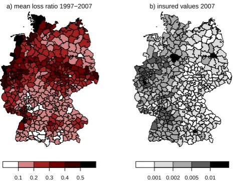
Fig. 3. Spatial distribution of the insurance loss data. (a) mean
winter half year loss ratios (VGV, years 1997–2007), normalised with loss ratio sum of all 439 administrative districts (unit: %) (b) insured values for the year 2007, normalised with total sum of all 439 administrative districts.
higher in the first than in the second region. Note that the normalisation of wind speeds relative to the local extreme wind climatology (represented by the 98th percentile) leads to a spatial smoothing of the hazard fields in comparison to the absolute wind speeds. This is also true in the case of high-resolution wind fields as provided by regional climate models, for example. The slope of the regression shows a strong relation to the mean losses (compare Fig. 3a), as may be expected since it is used to scale the wind-based loss po-tential towards observed loss amounts. However, the tempo-ral variability of the calculated losses is determined by the cubic wind term.
To calculate the Germany-wide loss ratio, the losses in the individual regions are added up, weighted by the locally in-sured sum (Fig. 3b).
cumulated loss ratio(event)= Germany
P
regions
value(region)·loss ratio(region,event)
Germany P
regions
value(region,year)
(4)
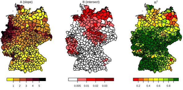
The local regression coefficients determined for loss calcu-lations (based on ERA-Interim gust wind speeds, for exam-ple) are presented in Fig. 4. Distinct regional differences are apparent, in particular, considering the slope of the regres-sion A. This coefficient may be interpreted as a measure for the local loss sensitivity to wind storm. High (low) values denote a strong (weak) increase of losses for higher wind speeds. The highest values are found in the north-western
part of Germany, particularly in the federal state of North Rhine-Westphalia, whereas the lowest values occur in the eastern and southern parts of Germany. The axis intercept B is generally close to zero when the regression is calculated on the basis of storm events. If the regression were to be cal-culated on the basis of annual loss sums, larger magnitudes of B would be apparent. This may be interpreted as a basic loss ratio accounting for losses emerging on days when no extreme wind speeds (exceeding the local 98th percentile) occurred. The coefficient of determinationR2exceeds 0.7 in most areas (Fig. 4, right panel), which means that the linear regression explains the largest part of the variance of losses. Lower values ofR2 down to about 0.2 are locally found in the south-eastern and north-eastern parts of Germany. The R2average over all districts is 0.78, confirming a generally well-determined link between losses and cubic wind speeds. The regional regression coefficients may differ for the cal-culation of losses based on the different wind datasets, in particular, with regard to the magnitudes of the coefficients. The basic pattern showing higher values of A for the north-western parts of Germany is, however, common to the regres-sions on the basis of all different wind data considered. A specific feature of the loss calculations on the basis of NCEP winds are some districts in the central eastern parts of Ger-many, where comparatively high values for the coefficient A are found (not shown). Here, the storms “Jeanett” and “Kyrill” caused high losses (compare Fig. 6, upper row), but the relatively coarse-resolution NCEP model does not pro-duce sufficiently high wind speeds in this region during these storms. This is consequently compensated by a steeper slope of the regression.
3.2 Loss calculations for severe storm events
A (slope)
1 2 3 4 5
B (intersect)
0.005 0.01 0.02 0.03
R2
0.2 0.4 0.6 0.8
Fig. 4. Regression coefficients for scaling the local loss potentials calculated from ERA-Interim gust wind speeds towards the insurance
loss records (VGV). Left: slope of the linear regression (coefficientA). Middle: axis intercept (coefficientB). Right: coefficient of determination (R2).
“Lothar” was characterised by extremely high wind speeds and related losses restricted to the southern part of Germany. Thus, maximum local losses were reached during “Lothar” (highest loss ratio in a district: 1.38 ‰), and local losses are somewhat smaller for the other two events (up to 1.19 ‰ for “Kyrill” and 0.43 ‰ for “Jeanett”). Also, other events may have caused severe local losses in specific regions, but from the cumulative point of view, losses during the three major events exceed those in the other loss events by about one or-der of magnitude. Although some differences are apparent for the most destructive events, the cumulated losses based on the VGV and VGV Sim insurance data generally agree well.
In general, the losses calculated from the different reanal-ysis wind fields reproduce the insurance data well (Fig. 5a). For storm “Kyrill” the losses are underestimated by all wind datasets by about 15 to 20 % in comparison to the VGV loss records, but are comparable to losses based on VGV Sim. Underestimation of the most severe events may be partly ex-plained by the specific regulation practices of some insur-ance companies: to manage the large numbers of claims after very loss-intensive events, companies often perform simpli-fied and optimised loss adjustment processes. This may con-tribute to disproportionately high loss values for some major events. However, owing to economic self-interest and regula-tory conditions, the insurance companies are obliged to reg-ulate the losses adequately and in accordance with the terms of insurance. Another contribution may come from demand surge effects after large events, i.e., the increase in costs for construction materials and labour as a consequence of the in-creased demand (Pielke Jr. et al., 2008; Olsen and Porter, 2011). Those company-specific and socio-economic effects are not accounted for by the loss model approach presented here. Nor does the loss model account for additional me-teorological parameters (such as heavy precipitation, small-scale turbulence, storm duration) which may have an effect on the loss amount.
Differences are also found for some weaker events (Fig. 5b), which are overestimated by individual reanaly-sis wind datasets (e.g., storms “Daniela”, “Ulf”, “Oratia”, “Noah”). These anomalies are, however, not systematic for the different reanalysis data and are generally explained by specific realisations of the storms with respect to intensity and area affected in the different datasets. The loss calcula-tions based on NCEP strongly underestimate the two major storms “Lothar” and “Jeanett”. In particular, the anomalies for the first reveal a peculiarity of the NCEP data. “Lothar” was a relatively small-scale secondary depression associ-ated with a strong steering cyclone (Ulbrich et al., 2001) which deepened explosively over the eastern Atlantic close to Europe and caused extremely severe damage over France, Switzerland and the southern parts of Germany. The coarse-resolution NCEP model does not capture this small cyclone system and, hence, fails to simulate the extremely high wind speeds leading to losses in southern Germany. For “Jeanett”, NCEP simulates too low wind speeds in many regions and particularly over the central parts of Germany. Nevertheless, NCEP provides a plausible picture of losses for most events. Apart from the described discrepancies, the use of these data is particularly advantageous for this study as they cover a pe-riod of more than 60 years, forming a robust basis for the estimation of return periods of severe storms (see Sect. 4).
2828 M. G. Donat et al.: High-resolution refinement of a storm loss model
(a)
K
y
rill
Lothar Jeanett Anna
Jennif
er
Anatol
Xylia−Winnie
Or
alie
Elvir
a−F
ar
ah
Sonja Dor
ian
Queenie Daniela
F
ann
y
Erwin
Ulf
Calv
ann Lar
a
K
erstin Or
atia
Heidi
Gerda−Hanna
Noah Ingo Ariane Her
ta
Natascha
Zar
ah
Ursula
Pia−Quimb
urga Britta Ilse
Maren Wisia
VGV VGV_Sim ERA−Int_wimax ERA−Int_gust NCEP
Loss Ratio
0.00
0.05
0.10
0.15
0.20
0.25
(b)
K
y
rill
Lothar Jeanett Anna
Jennif
er
Anatol
Xylia−Winnie
Or
alie
Elvir
a−F
ar
ah
Sonja Dor
ian
Queenie Daniela
F
ann
y
Erwin
Ulf
Calv
ann Lar
a
K
erstin Oratia Heidi
Gerda−Hanna
Noah Ingo Ariane Her
ta
Natascha
Zar
ah
Ursula
Pia−Quimb
urga Britta Ilse Maren Wisia VGV_Sim ERA−Int_wimax ERA−Int_gust NCEP
Diff
erence vs
. V
G
V
−0.10
−0.05
0.00
0.05
0.10
Fig. 5. Germany-wide cumulated losses for the 34 major loss events in the period 1997–2007 used for calibration of the loss model (unit: ‰). (a) For each event, the loss ratio is displayed on the basis of insurance losses to residential buildings (VGV, black bar), derived from vehicle
insurance data (VGV Sim, red bar), and calculated from the different reanalysis wind data: ERA-Interim maximum wind speed (grey), ERA-Interim maximum gust (purple), and NCEP maximum wind speeds (green). The losses for ERA-Interim and NCEP are calculated based on linear regressions derived from the other 33 events, excluding this particular storm.
(b) Difference of calculated storm losses relative to the VGV loss sums.
In general, the results confirm the ability of the loss model to realistically calculate both country-wide cumulated losses and also the spatial distribution of losses for severe storm events in Germany. However, the quality of the loss estimates depends on the meteorological input data. The results are particularly satisfactory for losses calculated from the ERA-Interim reanalysis, which is produced on a high spatial res-olution of approximately 0.7◦×0.7◦. Reasonable results are obtained for the NCEP reanalysis although it fails to repre-sent one of the most destructive storm events (owing to its coarse model resolution).
4 Estimation of return periods of loss-intensive wind storm events
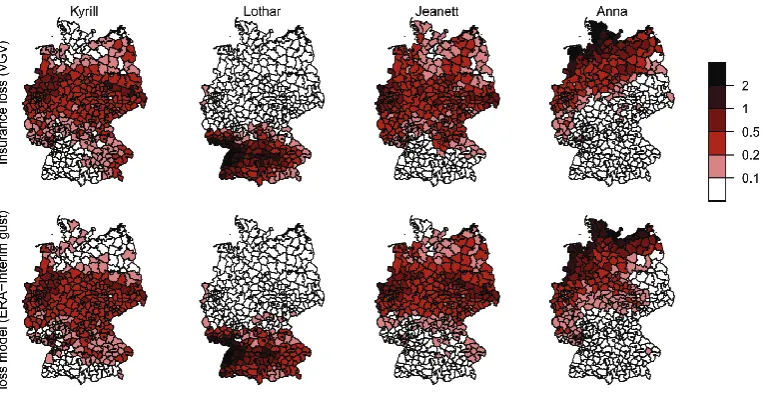
Fig. 6. Spatial distribution of losses for the four most loss-intensive single events in the period 1997 to 2007: insurance data (top row) and
calculated losses by applying the loss model to ERA-Interim gust (bottom row). For each event the local losses were calculated using the linear regression derived from the other 33 events, leaving out the particular storm itself. For each administrative district the loss ratio is shown relative to the country-wide cumulated loss for the specific event (unit: %).
data, and provides loss information back to 1948 when ap-plying the refined loss model to NCEP reanalysis (Table 3). The loss events are identified based on five day running sums of daily loss data (see Sect. 2.3).
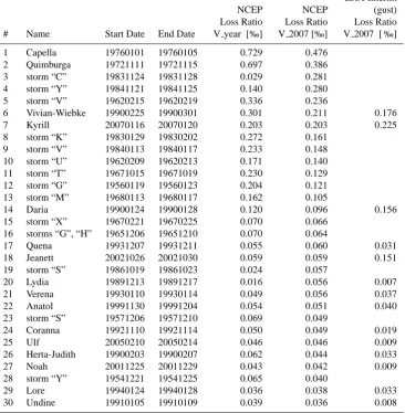
Extraordinarily severe loss events occurred in early 1990, for example, storms “Daria”, “Vivian” and “Wiebke”, and also in earlier decades in the second half of the 20th century. The most loss-intensive events in Germany during the recent 60 years identified here occurred in Jan 1976 (“Capella”), Nov 1972 (cyclone “Quimburga”, the “Lower Saxony Gale”, see Cappel and Emmerich, 1975) and Feb 1962 (a severe storm, causing a storm surge and leading to severe flood-ing in the city of Hamburg). Note that different reanalyses consistently suggest upward trends in the occurrence of win-ter storms in Central Europe for the second half of the 20th century, and also since the late 19th century (Donat et al., 2011b).
A considerable socio-economic uncertainty, related to dif-ferent spatial distributions of insured values, is apparent from the loss calculations based on NCEP. This effect is particu-larly strong for losses in earlier years. Cumulated losses for Germany were calculated using the spatial distribution of in-sured values (available for the years 1981 to 2007) of the specific year (Table 3, column 5), or using the most recent available value distribution (year 2007, column 6 in Table 3). The distribution of insured values is used for weighting the local losses when calculating cumulated losses for Germany. For years prior to approximately 2000, however, these data are affected by a number of uncertainties related to lower insurance density or less detailed reporting of losses. The distribution of values may, therefore, not be representative
for the earlier insurance data. For the eastern parts of Ger-many – the area of the former German Democratic Republic – insurance data are only available for years after 1990, and hence local losses are not accounted for when calculating cu-mulated losses for Germany. Furthermore, even for the other regions, information on insured values is only available back to 1981, and the value distribution of this year is, thus, also used when calculating cumulated losses in earlier years. Ow-ing to the wide range of difficulties with the early insurance portfolio data, we decided to consider the cumulated losses using the most recent value distribution of the year 2007 for the extreme value analysis in this section. This means that the insured values in the Landkreise remained constant for the NCEP-based return period estimation, which potentially dis-torts the cumulated losses in their historical context. These loss estimates indicate the losses that the historical storms would cause if they occurred under today’s socio-economic conditions rather than the losses in their historical context, and describe a possibility to normalise the losses to a ho-mogeneous portfolio. Also note the partly large differences between the NCEP and ERA-Interim based loss estimates for some individual events. These disparities reflect the dif-ferences in the realisations of these storms in the different reanalysis models and may partly also be related to the rel-atively coarse resolution of the NCEP model. On average, losses calculated from ERA-Interim showed a better agree-ment with insurance records for the period 1997–2007 com-pared to losses calculated from NCEP (see Sect. 3.2).
2830 M. G. Donat et al.: High-resolution refinement of a storm loss model
Table 2. The 30 most loss-intensive winter storm events
identi-fied from VGV Sim insurance records 1984–2008 and the associ-ated 5-day periods. The names of the associassoci-ated cyclones are indi-cated, start and end date of the five-day periods, and Germany-wide loss ratio sum for this period. Note that before 1990 cyclones were mostly denoted only by capital letters.
Loss Ratio
# Name Start Date End Date [‰]
1 Vivian-Wiebke 19900225 19900301 0.230
2 Kyrill 20070117 20070121 0.199
3 Daria 19900124 19900128 0.178
4 Lothar 19991223 19991227 0.123
5 Jeanett 20021025 20021029 0.118
6 Herta-Judith 19900203 19900207 0.072
7 Storm “Y” 19841122 19841126 0.066
8 Emma 20080299 20080303 0.040
9 Lore 19940125 19940129 0.039
10 storm “D” 19861019 19861023 0.038
11 Ismene 19921124 19921128 0.037
12 Verena 19930111 19930115 0.037
13 Coranna 19921109 19921113 0.035
14 Anatol 19991131 19991204 0.035
15 Quena 19931207 19931211 0.029
16 Wilma 19950122 19950126 0.029
17 Jennifer 20020125 20020129 0.027
18 Anna 20020223 20020227 0.026
19 Sonja 19970326 19970330 0.024
20 Elvira-Farah 19980303 19980307 0.022
21 Xylia 19981025 19981029 0.022
22 Oralie 20040319 20040323 0.021
23 storms “U”, “V” 19840113 19840117 0.020
24 Dorian 20051215 20051219 0.020
25 Daniela 19970217 19970221 0.019
26 storms “U”, “V” 19861215 19861219 0.018
27 Hetty 19980103 19980107 0.014
28 Erwin 20050106 20050110 0.013
29 Queenie 20040129 20040202 0.012
30 Ottilie-Pollie 19900211 19900215 0.012
in particular, the VGV insurance data are rather sparse with respect to a sound estimation of return periods, the curves for the different loss datasets agree remarkably well. The re-turn levels are highest (lowest) for the insurance-data-based fits for VGV Sim (VGV), flanking the curves for losses cal-culated from the two reanalysis datasets. The confidence in-tervals are narrowest for fits based on the long loss dataset calculated from NCEP reanalysis from 1948 to 2009. The good agreement between the different datasets suggests a high level of robustness of the return period estimates pre-sented here.
The extreme value analysis of the different loss datasets reveals that the return period of storm “Kyrill” (the most se-vere event in the VGV data 1997–2007, Germany-wide accu-mulated loss ratio approximately 0.24 ‰) is 15 years (based
0.5 1.0 2.0 5.0 10.0 20.0 50.0
0.0
0.1
0.2
0.3
0.4
0.5
Return Period [years]
Loss Ratio
VGV VGV_Sim ERA−Int NCEP
Fig. 7. Return period (unit: years) vs. return level (loss ratio, unit:
‰) plot for loss ratios based on the different loss datasets: VGV (black), VGV Sim (red), losses calculated based on ERA-Interim
gust (purple) and NCEP (green). Points indicate the empirical
dis-tribution, the solid lines the GPD best fits, the blue dashed lines the 95 % confidence interval (Profile Log-Likelihood Method) for the fit based on NCEP losses.
on the GPD fit for the VGV Sim data), 17 to 18 years (for losses calculated from both ERA-Interim and NCEP), and 21 years (VGV). The statistical uncertainty, expressed by the 95 % confidence interval (Profile Log-Likelihood Method recommended by Coles, 2001) related to the GPD-fit of the NCEP-based storm losses between 1948 and 2009, ranges between 9 and 43 years. The estimated return periods of the most loss-intensive storms since 1948 – ‘Capella’ in 1976 (loss ratio calculated from NCEP using the most re-cent distribution of values: 0.476 ‰) and “Quimburga” in 1972 (NCEP loss ratio: 0.386 ‰) – range between 29 and 45 years in the different datasets (95 % confidence interval between 15 and 145 years) for the first and 24 to 35 (95 % confidence interval between 13 and 100 years) years for the second. Conversely, the expected Germany-wide loss ratio for a 10-year event ranges between 0.12 ‰ and 0.16 ‰ based on the fits for the different loss datasets (95 % statistical con-fidence between 0.10 ‰ and 0.29 ‰), and for a 25-year loss event between 0.28 ‰ and 0.41 ‰ (95 % confidence between 0.17 ‰ and 0.85 ‰). For losses related to a 50-year storm event, the different fits already display a considerable spread, the expected loss ratios range between 0.52 ‰ (VGV) and 0.85 ‰ (VGV Sim), and the statistical uncertainty ranges from 0.26 ‰ to 1.93 ‰.
Table 3. Same as Table 2, but for storm events identified by applying the loss model to NCEP reanalysis (1948–2009). For those storms
occurring since 1989, the respective loss calculated based on ERA-Interim (gust) is also shown. Loss ratios were calculated using the distribution of values for the specific year (column “Loss Ratio V year”, see explanations in the text) and the most recent value distribution (i.e., 2007, column “Loss Ratio V 2007”).
ERA-Interim
NCEP NCEP (gust)
Loss Ratio Loss Ratio Loss Ratio
# Name Start Date End Date V year [‰] V 2007 [‰] V 2007 [ ‰]
1 Capella 19760101 19760105 0.729 0.476
2 Quimburga 19721111 19721115 0.697 0.386
3 storm “C” 19831124 19831128 0.029 0.281
4 storm “Y” 19841121 19841125 0.140 0.280
5 storm “V” 19620215 19620219 0.336 0.236
6 Vivian-Wiebke 19900225 19900301 0.301 0.211 0.176
7 Kyrill 20070116 20070120 0.203 0.203 0.225
8 storm “K” 19830129 19830202 0.272 0.161
9 storm “V” 19840113 19840117 0.233 0.148
10 storm “U” 19620209 19620213 0.171 0.140
11 storm “T” 19671015 19671019 0.230 0.129
12 storm “G” 19560119 19560123 0.204 0.121
13 storm “M” 19680113 19680117 0.162 0.105
14 Daria 19900124 19900128 0.120 0.096 0.156
15 storm “X” 19670221 19670225 0.070 0.066
16 storms “G”, “H” 19651206 19651210 0.070 0.064
17 Quena 19931207 19931211 0.055 0.060 0.031
18 Jeanett 20021026 20021030 0.059 0.059 0.151
19 storm “S” 19861019 19861023 0.024 0.057
20 Lydia 19891213 19891217 0.016 0.056 0.007
21 Verena 19930110 19930114 0.049 0.056 0.037
22 Anatol 19991130 19991204 0.054 0.051 0.040
23 storm “S” 19571206 19571210 0.069 0.049
24 Coranna 19921110 19921114 0.050 0.049 0.019
25 Ulf 20050210 20050214 0.046 0.046 0.009
26 Herta-Judith 19900203 19900207 0.062 0.044 0.033
27 Noah 20011225 20011229 0.043 0.042 0.009
28 storm “Y” 19541221 19541225 0.065 0.040
29 Lore 19940124 19940128 0.036 0.038 0.033
30 Undine 19910105 19910109 0.039 0.036 0.008
This scenario is, however, unrealistic because even when assuming total destruction of all buildings in the area consid-ered, the total sum of values is finite. In the case of total de-struction, a loss ratio equal to 1 would be expected. Note that the cumulated losses for the most destructive storm events in the past decades are in a co-domain of below approximately 0.5 ‰, i.e., only a small fraction of the total insured values. For losses in this dimension, the GPD fits for the different datasets display reasonable and stable results, thus, giving a certain amount of confidence in the return period estimation presented above.
5 Summary, discussion and conclusions
2832 M. G. Donat et al.: High-resolution refinement of a storm loss model by means of extreme value analysis. A GPD is fitted to the
losses for the severe storm events to estimate return periods of loss-intensive storms under current climate conditions. As a result, for example, the return period of losses caused by the storm “Kyrill” in 2007 is found to be about 15 to 21 years, depending on the individual dataset considered. “Capella”, the most loss-intensive storm considered here, is assumed to have a return period of 29 to 45 years.
Previous studies used a rather general approach for the cal-culation of losses (Klawa and Ulbrich, 2003; Leckebusch et al., 2007; Pinto et al., 2007; Donat et al., 2010a, 2011a), in particular a nationwide regression between wind speed and losses. This study also confirms the local applicability of the relatively simple basic assumptions on which the loss model is based: occurrence of losses for wind speeds exceeding the local 98th percentile and a cubic relationship between wind and loss. The latter is also reasonable in physical terms, as the cube of wind speed is proportional to the wind power. In addition, this study shows a specific benefit accruing from the inclusion of regionally specific loss characteristics. The main advantage of the loss model approach presented here is that it considers regional losses for single storm events, thus permitting improved estimates also of cumulated losses.
Nevertheless, the loss calculations may potentially be affected by several sources of uncertainty. First, socio-economic effects may influence the results. It was shown that assuming different spatial distributions of insured values leads to considerably different cumulated losses, particularly for pre-1991 storms (before 1991 information on insured values is only available for the western parts of Germany). Moreover, socio-economic effects regarding the amplifica-tion of losses in terms of increasing costs after large events are not accounted for in this study. Second, the meteorolog-ical data used to calculate losses contain uncertainties and partly do not even capture specific events. Although this may lead to substantial differences when calculating the losses for individual storms, the extreme value analysis results are very similar for the different loss datasets, suggesting a reason-able degree of robustness of the return period estimations presented here. Third, though they are subject to intensive quality control and provide a plausible picture of the losses, the insurance data may contain some imprecision. Different insurance companies (with generally different regional foci) often process the loss data differently, and the homogeneity of the loss records may be impaired by changes in insurance density or insured values or by fusions of companies, for ex-ample. Nevertheless, the GDV loss data are the best available loss dataset for the purpose of this study, and are used here as the reference data with respect to storm losses. At least since the turn of the millennium, the GDV data comprise more than 90 % of the German residential insurance market, so specific effects with individual insurers should counterbalance each other in the large sample. Fourth, there is also considerable statistical uncertainty obvious from the relatively wide con-fidence intervals of the GPD fit estimates, in particular for
long return periods above approximately 25 years. Reducing this uncertainty requires larger samples of storm loss data by including longer datasets of wind speed, for example, or by using ensemble simulations (Della-Marta et al., 2010; Donat et al., 2010b).
On the basis of extreme wind indices, Della-Marta et al. (2009) estimated the return periods of prominent wind storms from a Europe-wide perspective and found a large spread of the results, depending on the specific wind param-eter considered. The results in this study are restricted to loss amounts in Germany, but for most events the derived return periods are in a comparable order of magnitude.
Although our results suggest that infinitely high losses may occur, this is not realistic, as at least the existing val-ues limit the loss. The loss ratios for the most destructive historical events are, however, only a small fraction of the to-tal values, generally below 0.5 ‰. Our estimations are valid for losses in this order of magnitude, and the good agreement between the analyses based on the different datasets suggests a high confidence in the results.
The loss model was applied to reanalysis data in this study, but it can also be used to calculate storm losses based on climate model simulations. This should potentially com-plement previous studies estimating changes of loss under human-induced climate change conditions making use of a more general loss calculation approach. Explicitly account-ing for regional loss characteristics will allow more accurate estimates of possible future developments. Making use of high-resolution wind fields as simulated by regional climate models may further improve the skill of the loss estimations (Donat et al., 2010a).
Acknowledgements. This study was supported by the
Gesamtver-band der Deutschen Versicherungswirtschaft (GDV). We thank the European Centre for Medium-Range Weather Forecasts (ECMWF) and Deutscher Wetterdienst (DWD) for making ERA-Interim reanalysis data available. NCEP Reanalysis data were obtained from the NOAA/OAR/ESRL PSD, Boulder, Colorado, USA, from their web site at http://www.esrl.noaa.gov/psd/. We would like to thank Mareike Schuster for verifying the identified storm events in comparison to historical weather maps and we are grateful for the helpful comments provided by the two reviewers.
Edited by: O. Katz
Reviewed by: C. Etienne and another anonymous referee
References
Berliner Wetterkarte: published by Verein Berliner Wetterkarte e.V., ISSN 0177–3984, http://www.berlinerwetterkarte.de, 2009. Brodin, E. and Rootzen, H.: Univariate and
bivari-ate GPD methods for predicting extreme wind storm losses, Insur Math Econ, 44, 345–356, ISSN 0167-6687, doi:10.1016/j.insmatheco.2008.11.002, 2009.
Stuttgart, Reports of the German weather service, 135, Offen-bach, Germany, 1975.
Coles, S. G.: An Introduction to Statistical Modeling of Extreme Values, London, UK, Springer-Verlag, 224 pp., 2001.
Dee, D. P., Uppala, S. M., Simmons, A. J., Berrisford, P., Poli, P., Kobayashi, S., Andrae, U., Balmaseda, M. A., Balsamo, G., Bauer, P., Bechtold, P., Beljaars, A. C. M., van de Berg, L., Bid-lot, J., Bormann, N., Delsol, C., Dragani, R., Fuentes, M., Geer, A. J., Haimberger, L., Healy, S. B., Hersbach, H., H´olm, E. V., Isaksen, L., K˚allberg, P., K¨ohler, M., Matricardi, M., McNally, A. P., Monge-Sanz, B. M., Morcrette, J.-J., Park, B.-K., Peubey, C., de Rosnay, P., Tavolato, C., Th´epaut, J.-N. and Vitart, F.: The ERA-Interim reanalysis: configuration and performance of the data assimilation system, Q. J. Roy. Meteor. Soc., 137, 553–597, doi:10.1002/qj.828, 2011.
Della-Marta, P. M., Mathis, H., Frei, C., Liniger, M. A., Kleinn, J., and Appenzeller, C.: The return period of wind storms over Eu-rope, Int. J. Climatol., 29, 437–459, doi:10.1002/joc.1794, 2009. Della-Marta, P. M., Liniger, M. A., Appenzeller, C., Bresch, D. N., Koellner-Heck, P., and Muccione, V.: Improved estimates of the European winter wind storm climate and the risk of reinsurance loss using climate model data, J. Appl. Meteor. Climatol., 49, 2092–2120, doi:10.1175/2010JAMC2133.1, 2010.
Donat, M. G., Leckebusch, G. C., Wild, S., and Ulbrich, U.: Bene-fits and limitations of regional multi-model ensembles for storm loss estimations, Clim Res., 44, 211–225, doi:10.3354/cr00891, 2010a.
Donat, M. G., Leckebusch, G. C., Pinto, J. G., Ulbrich, U.: Euro-pean storminess and associated circulation weather types: future changes deduced from a multi-model ensemble of GCM simula-tions, Clim Res., 42, 27–43, doi:10.3354/cr00853, 2010b. Donat, M. G., Leckebusch, G. C., Wild, S., and Ulbrich,
U.: Future changes in European winter storm losses and ex-treme wind speeds inferred from GCM and RCM multi-model simulations, Nat. Hazards Earth Syst. Sci., 11, 1351–1370, doi:10.5194/nhess-11-1351-2011, 2011a.
Donat, M. G., Renggli, D., Wild, S., Alexander, L. V., Leckebusch, G. C., and Ulbrich, U.: Reanalysis suggests long-term upward trends in European storminess since 1871, Geophys. Res. Lett., 38, L14703, doi:10.1029/2011GL047995, 2011b.
Dorland, C., Tol, R. S. J., and Palutikof, J.: Vulnerability of the Netherlands and northwest Europe to storm damage under cli-mate change, Clim. Change, 43, 513–535, 1999.
ECMWF: IFS Documentation CY31r1, Part IV: Physical Processes, http://www.ecmwf.int/research/ifsdocs/CY31r1, 2007.
Fink, A. H., Br¨ucher, T., Ermert, V., Kr¨uger, A., and Pinto, J. G.: The European storm Kyrill in January 2007: synoptic evolu-tion, meteorological impacts and some considerations with re-spect to climate change, Nat. Hazards Earth Syst. Sci., 9, 405– 423, doi:10.5194/nhess-9-405-2009, 2009.
GDV: Yearbook 2006 – The German Insurance Industry, published by: Gesamtverband der Deutschen Versicherungswirtschaft e.V. (German Insurance Association), www.gdv.de, 2006.
GDV: Yearbook 2009 – The German Insurance Industry, published by: Gesamtverband der Deutschen Versicherungswirtschaft e.V. (German Insurance Association), www.gdv.de, 2009.
Heneka, P. and Hofherr, T.: Probabilistic winter storm risk assess-ment for residential buildings in Germany, Nat. Hazards, 56, 815–831, doi:10.1007/s11069-010-9593-7, 2011.
Heneka, P., Hofherr, T., Ruck, B., and Kottmeier, C.: Winter storm risk of residential structures model development and application to the German state of Baden-W¨urttemberg, Nat. Hazards Earth Syst. Sci., 6, 721–733, doi:10.5194/nhess-6-721-2006, 2006. Hofherr, T. and Kunz, M.: Extreme wind climatology of winter
storms in Germany, Clim. Res. 41, 105–123, 2010.
Kalnay, E., Kanamitsu, M., Kistler, R., Collins, W., Deaven, D., Gandin, L., Iredell, M., Saha, S., White, G., Woollen, J., Zhu, Y., Leetmaa, A., and Reynolds, R.: The NCEP/NCAR 40-year reanalysis project, Bull. Amer. Meteor. Soc., 77, 437–470, 1996. Kiss, P., Varga, L., and Ja`inosi, I. M.: Comparison of wind power estimates from the ECMWF reanalyses with direct turbine measurements, J. Renewable Sustainable Energy, 1, 033105, doi:10.1063/1.3153903, 2009.
Klawa, M. and Ulbrich, U.: A model for the estimation of storm losses and the identification of severe winter storms in Germany, Nat. Hazards Earth Syst. Sci., 3, 725–732, doi:10.5194/nhess-3-725-2003, 2003
Kunz, M., Mohr, S., Rauthe, M., Lux, R., and Kottmeier, Ch.: As-sessment of extreme wind speeds from Regional Climate Models - Part 1: Estimation of return values and their evaluation, Nat. Hazards Earth Syst. Sci., 10, 907–922, doi:10.5194/nhess-10-907-2010, 2010.
Leckebusch, G. C., Ulbrich, U., Fr¨ohlich, L., and Pinto, J. G.: Property loss potentials for European midlatitude storms in a changing climate, Geophys. Res. Let., 34, L05703, doi:10.1029/2006GL027663, 2007.
Olsen, A. H. and Porter, K. A.: What We Know about Demand Surge: a Brief Summary, Nat. Hazards Review, 12, 62–71, 2011. Palutikof, J. P. and Skellern, A. R.: Storm severity over Britain, a re-port to Commercial Union General Insurance. Climatic Research Unit, School of Environmental Sciences, University of East An-glia, Norwich, 1991.
Pielke Jr., R. A., Gratz, J., Landsea, C. W., Collins, D., Saunders, M., and Musulin, R.: Normalized Hurricane Damages in the United States: 1900-2005, Nat. Hazards Review, 9, 29–42, 2008. Pinto, J. G., Fr¨ohlich, E. L., Leckebusch, G. C., and Ulbrich, U.: Changing European storm loss potentials under modified climate conditions according to ensemble simulations of the ECHAM5/MPI-OM1 GCM, Nat. Hazards Earth Syst. Sci., 7, 165–175, doi:10.5194/nhess-7-165-2007, 2007.
Potsdamer Wetterkarte: Deutscher Zentralverlag GmbH, Berlin O 17, Verlagslizenz Nr. 363 – Gen.-Nr. 1006/48 – 32/48 (I) Paul D¨unnhaupt, K¨othen L, 77, 1949.
Shravan Kumar, M. and Anandan, V. K.: Comparision of the NCEP/NCAR Reanalysis II winds with those observed over a complex terrain in lower atmospheric boundary layer, Geophys. Res. Lett., 36, L01805, doi:10.1029/2008GL036246, 2009. Schwierz, C., K¨ollner-Heck, P., Zenklusen Mutter, E., Bresch, D.,
Vidale, P. L., Wild, M., and Sch¨ar, C.: Modelling European winter wind storm losses in current and future climate, Clim. Change, 101, doi:10.1007/s10584-009-9712-1, 2010.