University of Pennsylvania
ScholarlyCommons
Publicly Accessible Penn Dissertations
2012
Essays on Learning Under Ambiguity
Hongseok Choi
University of PennsylvaniaFollow this and additional works at:
https://repository.upenn.edu/edissertations
Part of the
Economics Commons
This paper is posted at ScholarlyCommons.https://repository.upenn.edu/edissertations/3216
For more information, please [email protected].
Recommended Citation
Choi, Hongseok, "Essays on Learning Under Ambiguity" (2012).Publicly Accessible Penn Dissertations. 3216.
Essays on Learning Under Ambiguity
Abstract
Over the past two decades, the growing literature on ambiguity aversion has shed light on a number of puzzles in financial economics. In most applications, however, a learning mechanism that maps observations toa posterioriambiguity is absent. Instead, a form of ambiguity known as IID ambiguity that is to model agents after they have learned all that they can has been the dominant specification in the literature. But when do we have the conjectured IID ambiguity? When does ambiguity resolve and when does it not? When it persists, what determines its long-run level and what are reasonable variations? In this dissertation, I provide answers to these questions by proposing a model of learning under ambiguity and investigate their implications for portfolio choice and asset pricing.
Specifically, I focus on the Gilboa-Schmeidler (1989) ambiguity aversion and assume that agents have the Chen-Epstein (2002) continuous-time recursive multiple-priors utility. Then, a learning mechanism means a map from each time-state to a set of one-step-ahead conditionals. I assume that the agents' beliefs about the data-generating mechanism are represented by multiple probabilistic models. As data accumulate, they assess the likelihood of each model, discard the ones with low likelihood, and update the remaining ones by Bayes' rule model-by-model. The dynamics of learning is explicitly characterized in the form of a system of
differential equations and I observe that in revising their estimates, agents take into account both the
uncertainty within each model and the uncertainty over the models. An application to portfolio choice shows that the effect of learning under ambiguity can be significant; the optimal weight on stocks monotonically decreases as the investor loses confidence and the decrease can be as large as 50\% of wealth. Finally, in an application to asset pricing, I make three observations regarding the equilibrium equity premium. First, learning under ambiguity generates a declining trend in the equity premium. Second, an improvement in the quality of signals can result in a higher equity premium. Third, the relationship between the equity premium and the conditional variance of returns is uncertain; they may be negatively correlated.
Degree Type
Dissertation
Degree Name
Doctor of Philosophy (PhD)
Graduate Group
Economics
First Advisor
Domenico Cuoco
Keywords
Subject Categories
ESSAYS ON LEARNING UNDER AMBIGUITY
Hongseok Choi
A DISSERTATION
in
Economics
Presented to the Faculties of the University of Pennsylvania
in
Partial Fulfillment of the Requirements for the
Degree of Doctor of Philosophy
2012
Supervisor of Dissertation
Domenico Cuoco, Associate Professor of Finance
Graduate Group Chairperson
Dirk Krueger, Professor of Economics
Dissertation Committee
Philipp Karl Illeditsch, Assistant Professor of Finance
ESSAYS ON LEARNING UNDER AMBIGUITY
c
COPYRIGHT
2012
ACKNOWLEDGEMENT
I owe my deepest gratitude to my advisor, Professor Domenico Cuoco, for his guidance and
support throughout the course of this research. He has spent an immeasurable amount of
time listening to his ignorant student, and I wish to state that those meetings with him
were not only enlightening but also the most enjoyable times I had in graduate school. I
was extremely lucky to have him as my advisor.
I would also like to thank Professor Philipp Illeditsch and Professor Dirk Krueger for
their guidance and support. I have much benefited from Professor Illeditsch’s expertise on
ambiguity aversion and Professor Krueger’s very constructive comments.
Most fundamentally, I would like to thank my parents for their unconditional support
ABSTRACT
ESSAYS ON LEARNING UNDER AMBIGUITY
Hongseok Choi
Domenico Cuoco
Over the past two decades, the growing literature on ambiguity aversion has shed light
on a number of puzzles in financial economics. In most applications, however, a learning
mechanism that maps observations to a posteriori ambiguity is absent. Instead, a form of
ambiguity known as IID ambiguity that is to model agents after they have learned all that
they can has been the dominant specification in the literature. But when do we have the
conjectured IID ambiguity? When does ambiguity resolve and when does it not? When
it persists, what determines its long-run level and what are reasonable variations? In this
dissertation, I provide answers to these questions by proposing a model of learning under
ambiguity and investigate their implications for portfolio choice and asset pricing.
Specifically, I focus on the Gilboa-Schmeidler (1989) ambiguity aversion and assume
that agents have the Chen-Epstein (2002) continuous-time recursive multiple-priors utility.
Then, a learning mechanism means a map from each time-state to a set of one-step-ahead
conditionals. I assume that the agents’ beliefs about the data-generating mechanism are
rep-resented by multiple probabilistic models. As data accumulate, they assess the likelihood of
each model, discard the ones with low likelihood, and update the remaining ones by Bayes’
rule model-by-model. The dynamics of learning is explicitly characterized in the form of a
system of differential equations and I observe that in revising their estimates, agents take
into account both the uncertainty within each model and the uncertainty over the models.
An application to portfolio choice shows that the effect of learning under ambiguity can
be significant; the optimal weight on stocks monotonically decreases as the investor loses
confidence and the decrease can be as large as 50% of wealth. Finally, in an application to
asset pricing, I make three observations regarding the equilibrium equity premium. First,
improvement in the quality of signals can result in a higher equity premium. Third, the
re-lationship between the equity premium and the conditional variance of returns is uncertain;
TABLE OF CONTENTS
ACKNOWLEDGEMENT . . . iii
ABSTRACT . . . iv
LIST OF FIGURES . . . viii
CHAPTER 1 : The Model of Learning under Ambiguity . . . 1
1.1 Introduction . . . 1
1.2 Preferences: Recursive Multiple-Priors . . . 5
1.3 Learning under Ambiguity: Preliminary Discussion . . . 7
1.4 The Theories . . . 12
1.5 The Utility Priors . . . 18
1.6 Discussion . . . 31
1.7 Proofs . . . 38
CHAPTER 2 : Consumption/Portfolio Choice . . . 58
2.1 Introduction . . . 58
2.2 The Setup . . . 58
2.3 Optimal Consumption and Portfolio . . . 62
2.4 Markovian Characterization . . . 64
2.5 Example . . . 67
2.6 Conclusion . . . 81
2.7 Proofs . . . 82
CHAPTER 3 : Asset Pricing . . . 86
3.1 Introduction . . . 86
3.3 Equilibria . . . 90
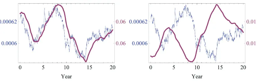
3.4 Declining Equity Premium & Rising Interest Rate . . . 93
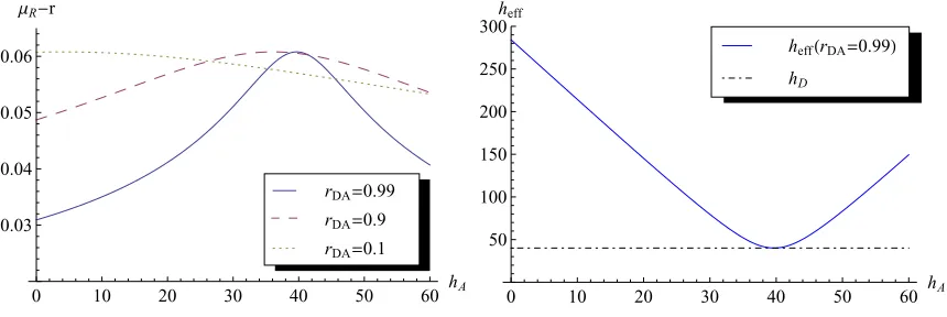
3.5 Equity Premium & Signal Precision . . . 95
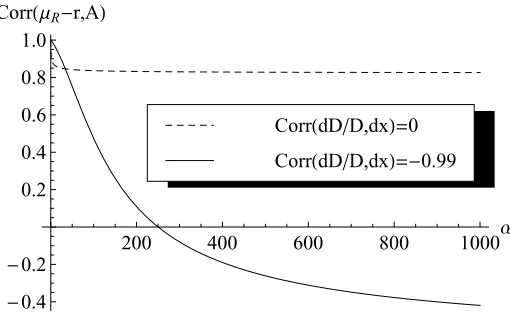
3.6 Equity Premium & Conditional Variance of Returns . . . 98
3.7 Proofs . . . 102
LIST OF FIGURES
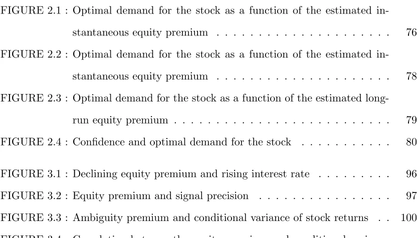
FIGURE 2.1 : Optimal demand for the stock as a function of the estimated
in-stantaneous equity premium . . . 76
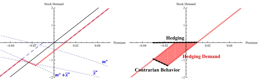
FIGURE 2.2 : Optimal demand for the stock as a function of the estimated in-stantaneous equity premium . . . 78
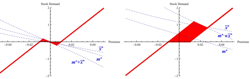
FIGURE 2.3 : Optimal demand for the stock as a function of the estimated long-run equity premium . . . 79
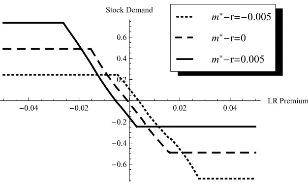
FIGURE 2.4 : Confidence and optimal demand for the stock . . . 80
FIGURE 3.1 : Declining equity premium and rising interest rate . . . 96
FIGURE 3.2 : Equity premium and signal precision . . . 97
FIGURE 3.3 : Ambiguity premium and conditional variance of stock returns . . 100
CHAPTER 1 : The Model of Learning under Ambiguity
1.1
Introduction
Standard models in financial economics assume that agents can form a unique probability
measure, called the prior, over uncertain investment opportunities. The uniqueness of the
prior in particular means that the agents can make probabilistic assessments of all relevant
uncertain events with infinite precision. More often than not, however, our knowledge
about the data-generating mechanism in question — for example, how stock returns are
generated — is limited and in such cases it is difficult to assess the likelihoods of uncertainties
precisely. In economics, Keynes (1921) and Knight (1921) were the first to recognize the
last possibility, and when an agent is modeled to be unable to form a unique prior, we say
there is Knightian uncertainty, or ambiguity.
Ambiguity is behaviorally distinct from risk. The simplest example is an ambiguous
coin (Ellsberg, 1961). Suppose there are two coins, where one is known to be fair; all that is
known about the other coin, on the other hand, is that it has two sides. Then, betting on the
fair coin would be preferred to betting on the ambiguous coin, which cannot be rationalized
by a subjective expected utility model. One resolution to Ellsberg-type paradoxes is Gilboa
and Schmeidler’s (1989) maxmin expected utility with nonunique prior, or multiple-priors
utility, and, over the past two decades, multiple-priors models have been used to explain a
number of puzzling phenomena in financial markets: stock market nonparticipation (Dow
and Werlang, 1992), excess volatility (Epstein and Wang, 1994; Illeditsch, 2011), excess
equity premium (Chen and Epstein, 2002), and equity home bias (Epstein and Miao, 2003),
to name a few.
In most applications, however, a learning mechanism that maps observations toa
poste-rioriambiguity is absent. Chen and Epstein (2002), who formulate a multiple-priors model
in continuous time, say, “the responsiveness to data permitted by our model is very general
and we do not yet have any compelling structure to add · · · to illustrate the response of
be explained later) form of ambiguity that they call independently and indistinguishably
distributed (IID) ambiguity, which is to model “the agent after he has learned all that
he can.” Ever since, IID ambiguity has been the dominant specification of ambiguity in
the literature. See Hern´andez-Hern´andez and Schied (2006, 2007a,b), Schied (2008), Miao
(2009), Routledge and Zin (2009), and Liu (2011) for applications of IID ambiguity to
port-folio choice and Epstein and Miao (2003), Trojani and Vanini (2004), and Gagliardini et al.
(2009) for those to asset pricing. Time-varying ambiguity without a learning mechanism has
been considered by Porchia (2005), Sbuelz and Trojani (2008), and Drechsler (forthcoming).
Naturally, the lack of a learning mechanism is unsatisfactory. For example, when do we
have the conjectured IID ambiguity? When does ambiguity resolve and when does it not?
When it persists, what determines its long-run level and what are reasonable variations?
These questions are important for their relevance to consumption/portfolio choice and asset
pricing. For example, in an economy populated by multiple-priors agents, the equilibrium
equity premium includes a premium for bearing ambiguity as well as the risk premium
and thus the specification of ambiguity has a direct effect on the level of and variations in
equity premia. In this dissertation, I provide answers to the above questions by proposing
a model of learning under ambiguity (Chapter 1) and investigate their implications for
consumption/portfolio choice (Chapter 2) and asset pricing (Chapter 3).
In Chapter 1, I define and solve the learning mechanism. Specifically, in this dissertation
I focus on the Gilboa-Schmeidler (1989) ambiguity aversion and assume that the agent
has the dynamic version of multiple-priors utility called recursive multiple-priors utility
(Epstein and Schneider, 2003b; Wang, 2003; Chen and Epstein, 2002). Then, the agent’s
beliefs are uniquely characterized by the sequence of the set of one-step-ahead conditionals
and a learning mechanism means a map from each time-state to a set of one-step-ahead
conditionals.
For concreteness, think of an agent who trades in the stock market. Due to limited
knowledge, he cannot narrow down his beliefs about how stock returns are generated to
probabilis-tic models. Specifically, the probabilisprobabilis-tic models the agent entertains are standard linear
state-space models (Liptser and Shiryaev, 1977, Chapter 12). The agent is certain that
the unobservable state, for example, the instantaneous expected return, is reverting to its
unconditional mean, but lacks confidence in the time-invariance of the latter. Accordingly,
he decomposes the unconditional mean into (i) a time-invariant component, for which he
entertains multiple marginal a prioridistributions, and (ii) a time-varying component that
he cannot model probabilistically (Epstein and Schneider, 2007; Walley and Fine, 1982). As
he observes stock returns, he (i) assesses the likelihood of each model, (ii) discards the ones
with low likelihood, and (iii) updates the remaining ones by Bayes’ rule model-by-model.
This gives him a set of one-step-ahead conditionals.
The main result of the chapter is an explicit characterization of the dynamics of learning
in the form of a system of differential equations. In the absence of ambiguity, the weight
on the innovation (unexpected changes in the observable variables) is increasing in the
Bayesian uncertainty in the estimates of the unobservable variables known as estimation
risk; the less trustworthy the current estimates, the more weight given on the new evidence.
I show that in the presence of ambiguity, the weight on the innovation is given by the
sum of estimation risk and a quantity that measures thea posteriorimodel uncertainty, or
estimation ambiguity. That is, in revising his estimates, the agent takes into account not
only the uncertainty within each model but also the uncertainty over the models.
Furthermore, estimation ambiguity persists if and only if the agent lacks confidence in
the time-invariance of the unconditional mean of the unobservable process. And when it
persists, I identify a necessary and sufficient condition for convergence to a constant, that
is, to an IID ambiguity, and compute the limit value; it is increasing in the agent’s lack of
confidence and conservatism in model selection and is decreasing in the variability of the
unobservable process relative to the observable process. In general, the filtering equations
allow us to study the endogenous relationship between the level of a posteriori ambiguity
and other primitives of the model like signal precision.
and is closely related to Epstein and Schneider (2007), who also construct the set of
one-step-ahead conditionals by a likelihood-ratio test over multiple probabilistic models. The
differences between their model and mine are as follows. First, whereas Epstein and
Schnei-der’s model is in discrete time, mine is in continuous time. The transition to continuous time
is more than a technical extension: the continuous-time counterpart of their portfolio choice
example results in no learning because the likelihood function degenerates to infinity
every-where (Section 1.3.3). Thus, in particular, their discrete-time finding that learning resolves
ambiguity does not immediately carry over to continuous time. Second, whereas Epstein
and Schneider focus on memoryless data-generating mechanisms, I consider path-dependent
ones, which clearly complements the former. For example, with the present model, we can
study the effects of learning under ambiguity when stock returns or the growth of dividends
is predictable (Chapter 2 and 3).1
Another paper that considers the learning of a recursive multiple-priors agent is Miao
(2009). Specifically, he considers the consumption/portfolio choice problem of an investor
in continuous time and allows for stochastic investment opportunities. However, his notion
of learning is fundamentally different from mine. Miao’s investor obtains the benchmark
step-ahead conditional by updating a reference probability measure and the set of
one-step-ahead conditionals is given by a neighborhood of the benchmark with a fixed radius.
Thus, in particular, learning and ambiguity do not interact. In fact, Miao’s model is the
limit of the present model as the investor gains confidence. See Section 2.5.3.2
The rest of Chapter 1 is organized as follows. In Section 1.2, I review Chen and Epstein’s
(2002) continuous-time recursive multiple-priors utility. Section 1.3 motivates the learning
mechanism to be discussed in the subsequent sections. Section 1.4 defines the probabilistic
models that the agent entertains. Section 1.5 defines and solves the learning mechanism.
Section 1.6 discusses the dynamics of learning. All proofs are collected in Section 1.7.
1
Campanale (2011) applies Epstein and Schneider’s (2007) model in the context of life-cycle portfolio choice and Miao and Wang (2011) in the context of job matching. Epstein and Schneider’s (2008) asset pricing model conforms to the formalism of Epstein and Schneider (2007) but their agents do not discard any of the models theya priorientertain. See also Knox (2002).
2
1.2
Preferences: Recursive Multiple-Priors
I assume that the agent has Chen and Epstein’s (2002) recursive multiple-priors utility.3
Specifically, time is continuous and varies over [0, T],T ∈(0,∞).
Let Ω denote the set of states of Nature and let a filtration G= {Gt} on Ω represent
the accrual of the agent’s information. Gis right-continuous.
There is a setP of equivalent probability measures on (Ω,GT), the set of priors, with the
following properties. LetP0∈ P. There is ann
y-dimensional Wiener process ={(t),Gt}
under P0 that generates G. (The notation = {(t),Gt} signifies that the process is
adapted to the filtration G. All vectors, including the gradient ∂f of a scalar function f,
are column vectors. Hence, (t) = (1(t),· · · , ny(t)) >.) G
0 contains all the P0-null events
in GT. Thus, in particular, G satisfies the usual conditions. Each prior is identified with
the corresponding density generator ξ={ξ(t),Gt} and is thus written Pξ ∈ P, where
dPξ dP0 =E
ξ(T) (1.1)
and Eξ denotes the Dol´eans-Dade exponential
Eξ(t),exp
Z t
0
ξ(s) d(s)−1 2
Z t
0
|ξ(s)|2ds
, 0≤t≤T.
P is required to be rectangular, which means that there is a set-valued process Ξ : [0, T]×
Ω→2Rny such that the probability measurePξ defined by (1.1) is a prior if and only ifξ
is a G-progressive process and ξ(t, ω)∈Ξ(t, ω) for Lebesgue×P0 almost every (t, ω). Since
P consists of equivalent measures, “for Lebesgue×P0 almost every (t, ω)” is henceforth
abbreviated without ambiguity to “a.e.” Ξ is called theone-step-ahead conditionals process
and is further required to be (i) uniformly bounded, (ii) compact-convex-valued, and (iii)
3
“G-progressive”: (i) Ξ(t, ω) ⊂K a.e. for some bounded K ⊂Rny, (ii) Ξ(t, ω) is
compact-convex a.e., and (iii) the restriction of Ξ to [0, t]×Ω is B[0, t]⊗ Gt-measurable4 for all
t∈[0, T] whereBX denotes the Borelσ-algebra of a topological space X.
A scalar process c = {c(t),Gt} is a consumption process if it is progressive, positive,
and integrable. Denote the set of consumption processes by C. The agent’s conditional
preferences at time t,t∈[0, T], are represented by
Uc(t, ω) = min P∈PU
c,P(t, ω), c∈ C (1.2)
where Uc,P = {Uc,P(s),G
s}, the utility process under P ∈ P, uniquely solves the BSDE
(backward stochastic differential equation)
Uc,P(s) = EP
Z T
s
F(c(τ), Uc,P(τ)) dτ
Gs
, t≤s≤T.
Here,F is the aggregator. See Chen and Epstein (2002), Section 2.5 for the conditions that
the aggregator has to satisfy.
Rectangularity is an essential requirement for the Epstein-Schneider-Wang recursive
representation and hence for their notion of dynamic consistency.5 The utility process Uc
defined by (1.2) satisfies
dUc(t) =
−F(c(t), Uc(t)) + max ξ(t)∈Ξ(t)σ
c U(t)ξ(t)
dt+σUc(t) d(t), 0≤t≤T (1.3)
with terminal conditionU(T) = 0, for some processσUc ={σUc(t),Gt}. When (1.3) is viewed
as a BSDE, the pair (Uc, σUc) constitutes a solution.
To interpret (1.3), rewrite it, with a slight abuse of notation, as
dUc(t) =−F(c(t), Uc(t)) dt+ max ξ(t)∈Ξ(t)σ
c
U(t)( d(t) +ξ(t) dt)
4{
(s, ω)∈[0, t]×Ω : Ξ(s, ω)∩K0 6=∅} ∈ B[0, t]⊗ Gt for all closed K0 ⊂K. See Aliprantis and Border
(1999), Sections 16.1, 16.2, and 17.1.
5
and compare it with the standard, single-prior stochastic differential utility representation
(Duffie and Epstein, 1992)
dUc(t) =−F(c(t), Uc(t)) dt+σUc(t) d(t).
Consider first the single-prior case. By the assumption that generates G, all changes in
the fundamentals to take place over the infinitesimal future are a function of d(t). In other
words, the agent’s conditional beliefs about the uncertainties to be resolved over the next
instant are summarized by the unique distributionN(0,dt) for the “one-step-ahead” noise
d(t). Now, the representation for the ambiguity-averse agent suggests the interpretation
that he entertains asetof plausible distributionsN(ξ(t),dt),ξ(t)∈Ξ(t). And a pessimist,
he assessesc under the belief that the distribution that is the worst forc is the case.6
1.3
Learning under Ambiguity: Preliminary Discussion
Modeling learning dynamics in the context of recursive multiple-priors amounts to
impos-ing a particular structure on the set of priors beyond rectangularity. Since a rectangular
set of priors uniquely determines a one-step-ahead conditionals process and vice versa, it
is equivalent to defining a map from an observation (t, ω) to a set of one-step-ahead
con-ditionals Ξ(t, ω), which is both conceptually and operationally preferable for the following
reasons. First, the set of one-step-ahead conditionals at a certain point in time precisely
models the agent’s conditional beliefs; in a Bayesian model, the map is the Bayesian
up-dating of the unique prior (followed by the restriction to the one-step-ahead information).
Second, the one-step-ahead conditionals process is essentially unrestricted; boundedness
and compact-convexity are intrinsic to the Gilboa-Schmeidler ambiguity and measurability
is merely technical. For these reasons, Epstein and Schneider (2007) call the one-step-ahead
conditionals process “a natural vehicle for modelling learning dynamics.”
In this section, I explain how I model the agent’s learning dynamics. The proposed
6
mechanism is closely related to Epstein and Schneider’s (2007) and it thus helps to briefly
review their model first.
1.3.1 Epstein and Schneider (2007)
Here I review Epstein and Schneider’s (2007) model of learning under ambiguity focusing
on their main example in which stock returns follow a binary process in discrete time.
Their model of stock returns formally corresponds to the robust Bernoulli model of
Walley (1991, Section 9.6). Begin with the standard, conditionally i.i.d. binary return
process. There is a stock for which there are d trading days per month. The likelihood
function for the net rate of return between two consecutive trading days is7
L
∆R(t) =±σR/ √
d
x¯
= 1 2 ±
1 2
¯ x σR
√ d
whereRdenotes the cumulative return process and the implied monthly expected return ¯x∈
Ris unknown. A Bayesian agent would have a unique parameter prior M (the marginal a
prioridistribution for the parameter ¯x) and learning would amount to the Bayesian updating
ofM. Epstein and Schneider introduce ambiguity by generalizing the exchangeable Bayesian
model in the following way. First, there are multiple parameter priors. Second, there are
multiple stepwise likelihood functions
L∆R(t) =±σR/ √
d
x, η(t)¯
= 1 2 ±
1 2
¯ x+η(t)
σR √
d , |η(t)| ≤η¯ (1.4)
for some ¯η <∞, so thatat each trading datet, any value ofη(t),|η(t)| ≤η, could be the case.¯
Thus, the assumption of identical distributions is replaced by the weaker exchangeability
assumption ofindistinguishable distributions (Epstein and Schneider, 2003a, 2007; Epstein
and Seo, 2010, 2011).
η(t) captures the factors of the data-generating mechanism the agent understands
poorly, no more than the bound |η(t)| ≤ η. Or an alternative interpretation is that the¯
agent doubts the assumption that the expected return is constant but is unable to formalize
7
it probabilistically. The key characteristics of the Walley-Epstein-Schneider generalization
are (i) η is nonparametric, that is, no connection of any sort is assumed between η(s) and
η(t), s6=t, and (ii) {η(t)} are incidental (Neyman and Scott, 1948), that is, the sequence
η={η(1), . . . , η(T)} grows with observation. Consequently,η is impossible to learn.
Based on the above generalization of the exchangeable Bayesian model, Epstein and
Schneider (2007) nonaxiomatically propose the following learning mechanism. Collect the
multiple parameter priors inMand the multiple stepwise likelihoods inL. Mmay consist
only of Dirac measures; to quote Epstein and Schneider, “Indeed, one may wonder whether
there is a need for non-Dirac priors at all.” Having observed the returns up to trading date
t > 0, the agent entertains all the data-generating mechanisms conceivable from the pair
(M,L), that is,M × Lt=M ×(L × · · · × L). Each (M, Lt)∈ M × Lt is called atheory.
Now, the agent rules out theories with low likelihood and Bayes-updates the remaining
ones to obtain the set of one-step-ahead conditionals: denoting the log-likelihood function
of theories by`t(M, Lt), the set of one-step-ahead conditionals is given by
Z
L(·|x, η(t¯ + 1)) dMt(M, Lt) :|η(t+ 1)| ≤η¯and `t(M, Lt)≥ max
(µ,λt)∈M×Lt`t(µ, λ t)−α
(1.5)
whereMt(M, Lt) denotes the posterior of ¯xobtained from (M, Lt) by Bayes’ rule andα ≥0
is a primitive. And from this, the set of priors is determined by backward induction.
1.3.2 Classical Updating Rule
Each theory defines a probability measure on the observation σ-algebra (the σ-algebra
generated by the return process). Note, however, that the set of the probability measures on
the observationσ-algebra implied by the theories are not necessarily the set of priors derived
from the theories by the learning mechanism described above; the former will typically be
smaller than the latter. This is the case even ifα=∞and no theories are discarded. That
is, if we elicit the beliefs of an agent who entertains multiple data-generating mechanisms
and at the same time behaves dynamically consistently in the sense of Epstein and Schneider
beliefs the agent actually has regarding the data-generating mechanism. To quote Epstein
and Schneider (2003b),
P0[an arbitrary set of probability measures that is thought to model the agent’s
beliefs] induces sets of one-step-ahead conditionals and these generate P [the
set of priors] as described above. Because induced one-step-ahead conditionals
are precisely what one needs to compute utility by backward induction, we can
view P as precisely the enlargement of P0 needed in order to incorporate the
logic of backward induction.
In unique-prior models, typically the two notions ofa prioribeliefs are considered, explicitly
or implicitly, one and the same.
Given the distinction, we may then speak of the updating of multiple theories. And
a natural way to learn under this interpretation, albeit not axiomatically incorporated to
recursive multiple-priors, is that of classical statistics: rule out theories with low likelihood
and update the remaining ones by Bayes’ rule. Gilboa and Schmeidler (1993) call this the
classical updating rule and axiomatize the extreme case, namely, the maximum-likelihood
classical updating rule. They show (i) it coincides with the pessimistic Bayesian updating
where the latter means that upon learning that an eventAhas occurred, the agent behaves
as if he believed that had A not occurred, the best possible outcome would have resulted,
and (ii) it is commutative in the sense that the conditional preferences givenA∩B are the
same whether it is obtained sequentially conditioning onB after onAor at once onA∩B.
There are two differences between Epstein and Schneider (2007) and the present
disser-tation in terms of modeling learning under ambiguity. First, Epstein and Schneider focus
on memoryless theories (recall (1.5)), whereas I consider path-dependent theories. Indeed,
the classical updating rule, or any selection-rule-based learning mechanism in general, is
applicable to any set of theories. Second, Epstein and Schneider’s model is in discrete time,
whereas I set up a continuous-time model. It turns out that the last difference is nontrivial.
If we take the continuous-time limit of their return process first and then apply their
degenerates to infinity everywhere. I turn to this point now.
1.3.3 Discrete Time versus Continuous Time
The continuous-time return process implied by (1.4) is
dR(t) = (¯x+η(t)) dt+σRdw(t) (1.6)
with|η(t)| ≤η¯for allt.8 The log-likelihood function of (¯x, η) is (see Proposition 1.3)
Z T
0
(¯x+η(t))σR−2dR(t)−1 2
Z T
0
[σ−R1(¯x+η(t))]2dt.
But the sequence {ην :ν= 1,2, . . .}defined by
ην(t),
0 ift= 0
+¯η ift∈(tνi, tνi+1] and R(tνi+1)−R(tνi)>0
−η¯ ift∈(tνi, tνi+1] and R(tνi+1)−R(tνi)≤0
where{tν1, . . . , tνν}is theνth dyadic partition of [0, T], will make the integralRT
0 η
ν(t) dR(t)
diverge to the infinite variation ofR.9 Epstein and Schneider could circumvent this problem
because the set of one-step-ahead conditionals (1.5) is well-defined for all trading frequencies
dand converges. But if time is continuous at the outset, such a circumvention is not possible.
To have a continuous-time model of learning under ambiguity, I relax the assumption
that the drift of the observable process is constant and let it be time-varying. Accordingly,
8Assumed→ ∞and observe that the mean of the return is
¯
x+η σR √ d σR √ d= ¯
x+η
d = (¯x+η) dt
and that the variance of the return is
σR √
d−
¯
x+η d 2 1 2+ 1 2 ¯
x+η σR √ d + −√σR
d−
¯
x+η d 2 1 2− 1 2 ¯
x+η σR √ d ≈ σ 2 R
d =σ
2 Rdt.
9
the agent now faces ambiguity regarding the dynamics of the hidden state. I show that in
this setup, a nondegenerate likelihood-ratio statistic can be defined.
1.4
The Theories
Denote the observable process that generates the agent’s information by y = {y(t),Gt}.
That is,Gis theP0-augmentation of the filtration generated byy. nydenotes the dimension
of y. Examples of y will be given shortly.
In this section, I define the theories that the agent entertains about howyis generated.
They are given by a set of probability measures Q∈ Q on a common measurable space.
1.4.1 The Reference Likelihood
Let there be a filtrationF={Ft} on Ω and a probability measureQx,¯0 on (Ω,FT) where
¯
x∈Rnx,nx≥1. Fsatisfies the usual conditions with respect toQ¯x,0. Let there also be two
independentQx,¯0-Wiener processesw={w(t),Ft}andvx,¯0 ={vx,¯0(t),Ft},ny-dimensional
and nx-dimensional, respectively. UnderQx,¯0,y satisfies the following system of SDEs:
dy(t) = (a(t, y) +b(t, y)x(t)) dt+σ(t, y) dw(t)
dx(t) =κx(¯x−x(t)) dt+ρwdw(t) +ρvdv¯x,0(t).
Here, x = {x(t),Ft} is an nx-dimensional process that is unobservable to the agent;
a : [0, T]×C([0, T],Rny) → Rny, b : [0, T]×C([0, T],Rny) → Rny×nx, and σ : [0, T]×
C([0, T],Rny)→Rny×ny are nonanticipating path functionals whereC([0, T],Rny) denotes
the set of continuous functions from [0, T] intoRny;10κxis annx×nx diagonal matrix with
positive entries,ρw is annx×ny matrix, andρv is annx×nx invertible matrix. Given that
y is observed, the diffusion matrix process σσ>, too, is observed via quadratic
variation-covariation. The assumption that σ as a nonanticipating path functional depends only on
y, or equivalently, σ as a process is adapted to G, embodies the restriction that observing
10
the diffusion matrix does not expand the agent’s information. x(0) is an F0-measurable
random variable. The distribution ofx(0) conditional onG0 is normal with meanm0∈Rnx
and variance-covariance matrix γ0 ∈Rnx×nx. For simplicity, I assume y(0) is nonrandom.
All the parameters and functional forms are known but ¯x.
Example 1.1 (Stock Returns with Constant Volatility). Suppose that the cumulative
re-turn processR of a stock satisfies
dR(t) =x(t) dt+σRdw(t)
and R is the only observable process. Then, y=R witha≡0,b≡1, and σ≡σR>0.
Example 1.2 (Stock Returns with Stochastic Volatility).Suppose that the conditional
return variance follows a Cox-Ingersoll-Ross process (Heston, 1993), that is,
dR(t) =x(t) dt+pA(t)(
q
1−rRA2 , rRA) dw(t)
dA(t) =κA( ¯A−A(t)) dt+ςA
p
A(t)(0,1) dw(t)
whererRA ∈(−1,1), κA>0,A¯∈R, andςA>0. Suppose also that R and A are the only
observable processes. Then,y= (R, A)> with
a(t, y) =
0
κA( ¯A−A(t))
, b≡
1
0
, and σ(t, y) = p
A(t)
q
1−r2
RA rRA
0 ςA
.
Example 1.3 (Extra Signal). Suppose that the return volatility is constant as in Example
1.1 but now there is an extra signal about the hidden state x in addition toR (Detemple,
1986; Veronesi, 2000):
dR(t) =x(t) dt+σR(
q
1−r2
RA, rRA) dw(t)
whererRA∈(−1,1)and σR, σA>0. Then,y= (R, A)> with
a≡
0
0
, b≡
1
1
, and σ≡
σR
q
1−r2RA σRrRA
0 σA
.
Similar examples can be constructed in a general equilibrium setting in which, for example,
the aggregate consumption growth replaces the stock returns.
Now, the reference likelihood function of the unknown parameter ¯x under full
observa-tion, or simply the reference likelihood, is defined by
LFO,T(¯x), dQx,¯0 dQ0,0.
1.4.2 Bayesian (Unique-Prior) Benchmark
Let M be a probability measure on (Rnx,BRnx). Then, (M, LFO,T) defines a standard
Bayesian model where (M, LFO,T) describes the data-generating mechanism according to
which ¯x is drawn fromM and conditional on ¯xthe law of (y, x) is given by LFO,T(¯x).
1.4.3 The Theories
Bayesian agents behave as if they knew the probabilities of all relevant events precisely.
Con-sider in contrast an agent who lacks confidence in his understanding of the data-generating
mechanism and finds both the parameter ¯x and the reference likelihoodLFO,T ambiguous.
Specifically, the agent’s perception of ambiguity regarding ¯x is expressed by the
multi-plicity of parameter priors. For simmulti-plicity, I assume that the set of parameter priors consists
only of Dirac measures:
M={Diracx¯0 : ¯x0 ∈Rnx}
where Diracx¯0 denotes the Dirac measure concentrated at ¯x0 ∈Rnx.
Similarly, the agent also entertains multiple likelihoods. Fix ¯x. Let there be a probability
measureQx,η¯ ,η∈L2([0, T],Rnx), on (Ω,FT) whereL2([0, T],Rnx) denotes the set of
{v¯x,η(t),Ft} independent ofw. UnderQx,η¯ , (y, x) satisfies the following system of SDEs:
dy(t) = (a(t, y) +b(t, y)x(t)) dt+σ(t, y) dw(t) (1.7)
dx(t) =κx(¯x−x(t)) dt+ρwdw(t) +ρv( dvx,η¯ (t) +η(t) dt) (1.8)
where, as before, y(0) ∈ Rny is nonrandom and the F0-measurable random variable x(0)
has the conditional distributionx(0)|G0 ∼N(m0, γ0). The set of full-observation likelihood
functions is given by
LFO,T =
¯
x7→LFO,T(¯x, η) :η ∈L2([0, T],Rnx)
LFO,T(¯x, η), dQx,η¯ dQ0,0.
Compare this specification of multiple likelihoods with Epstein and Schneider’s (2007)
reviewed in Section 1.3.1, that is, (1.4) and (1.6). As with theirs, the current specification
(1.7)-(1.8) also incorporates the notion of indistinguishability; η is nonparametric and the
only restriction of square-integrability is global. But while in (1.6) the agent’s lack of
confidence is expressed as the ambiguity in the drift of the measurement error process, in
(1.7)-(1.8) it is expressed as the ambiguity in the drift of the unobservable process. To give
an alternative interpretation ofη, we can rewrite (1.8) as
dx(t) =κx x¯+κ−x1ρvη(t)−x(t)
dt+ρwdw(t) +ρvdvx,η¯ (t).
That is, the agent lacks confidence in the time-invariance of the unconditional mean of x
and suspects the existence of a time-varying factorη that he cannot model probabilistically.
Now I turn to the issue of the existence and uniqueness of a solution to the system of
SDEs (1.7) and (1.8). | · |denotes the Euclidean norm for vectors and the Frobenius norm
for matrices; that is, for a vector or matrix z, |z|,ptr(zz>). All numbered assumptions
Assumption 1.1 (Sufficient Conditions for Unique Strong Existence).(i) b is uniformly
bounded.
(ii) For allf ∈C([0, T],Rny),
Z T
0
(|a(t, f)|+|σ(t, f)|2) dt <∞.
(iii) a,b, and σ are locally Lipschitz. That is, for eachN there is aKN such that
sup s≤t
|f(s)|
∨
sup s≤t
|g(s)|
≤N ⇒ |σ(t, f)−σ(t, g)| ≤KNsup s≤t
|f(s)−g(s)|
for all t∈[0, T]; and the same foraand b mutatis mutandis.
(iv)aand σ are linearly growing. That is, there is aK such that
|a(t, f)|+|σ(t, f)| ≤K 1 + sup t≤T
|f(t)|
!
for all (t, f)∈[0, T]×C([0, T],Rny).
Proposition 1.1.Strong existence and pathwise uniqueness hold for the system of SDEs
(1.7)-(1.8).
Suppose (w, vx,η¯ ) and (y, x) are defined on some filtered complete probability space.
With a slight abuse of notation, σ(t) ≡ σ(t, ω) ≡σ(t, y(ω)). With the notation σ(t, ω), σ
can be considered a process (adapted toG). Similar remarks apply to the other functionals.
As is the custom, the qualification almost surely is suppressed unless necessary.
Assumption 1.2.There is an ε >0 such that
Remark 1.1.The stochastic volatility model (Example 1.2) violates Assumption 1.2:
σ(t)σ(t)>=A(t)
1 rRAςA
ςArRA ςA2
and the last matrix that post-multiplies A(t) satisfies Assumption 1.2,11 butA(t) may get
arbitrarily close to 0. In general, if Assumption 1.2 fails, then the subsequent findings based
on the assumption hold up to the random time
T∧infnt >0 :z>σ(s)σ(s)>z≥N−1|z|2 for all z∈Rny and alls≤to.
Assumption 1.2 implies that σ(t) has an inverse and |σ(t)−1z| ≤ K−1/2|z|for all z ∈
Rny
and all t ∈ [0, T]; likewise, σ(t)>, too, has an inverse and |(σ(t)>)−1z| ≤ K−1/2|z| for all
z ∈ Rny and all t ∈ [0, T] (Karatzas and Shreve (1988), Problem 5.8.1). With the last
observation, we can rewrite (1.7) and (1.8) as
dw(t) =σ(t)−1[ dy(t)−(a(t) +b(t)x(t)) dt] (1.9)
dvx,η¯ (t) =ρ−v1
dx(t)−κx(¯x−x(t)) dt−ρwσ(t)−1[ dy(t)−(a(t) +b(t)x(t)) dt] −η(t) dt
(1.10)
and use these SDEs to definew andvx,η¯ .
Let
Ω,C([0, T],Rny)×C([0, T],Rnx)
11The question is if there is a (small)ε >0 such that for allz= (z 1, z2),
0≤z12+ 2z1z2ςArRA+z22ς 2 A−ε(z
2 1+z
2 2)
= (1−ε)
z1+
z2ςArRA
1−ε
2 −
z2ςArRA
1−ε
2
+z22
ςA2 −ςA
1−ε
!
.
The last inequality holds for allz if and only if
ςA2(1−ε−r 2
RA)≥ε(1−ε).
F◦ ,BC([0, T],Rny)⊗ BC([0, T],Rnx),
let (y, x) be the identity map on Ω, and let
Qx,η¯ ,law(y, x)
be defined on (Ω,F◦). LetF={Ft}be the augmented filtration generated by (y, x). Since
Qx,η¯ , (¯x, η)∈Rnx×L2([0, T],Rnx), are equivalent, they all lead to the same augmentation.
Finally, define σ by σ(t, ω) = σ(t, y(ω)) and define w and vx,η¯ by (1.9) and (1.10). In
particular, this construction (of weak solutions) explains whyv¯x,η is superscripted.
In sum, the agent’s theories of how the data y is generated can be identified with the
probability measures
Q,
Q¯x,η: (¯x, η)∈Rnx×L2([0, T],Rnx)
on the common measurable space (Ω,FT), all defined above. I call these probability
mea-sures data priors to distinguish them from the probability measures P ∈ P that are
part of the representation of the agent’s preferences, or the utility priors. Not only are
these two types of priors conceptually distinct, but they are different; we will see that
P *{Q|GT :Q∈ Q} whereQ|GT denotes the restriction ofQ toGT.
1.5
The Utility Priors
1.5.1 Filtering
Recall the partially observable system
dy(t) = (a(t) +b(t)x(t)) dt+σ(t) dw(t) (1.11)
dx(t) =κx(¯x−x(t)) dt+ρwdw(t) +ρv( dvx,η¯ (t) +η(t) dt). (1.12)
Proposition 1.2.The following standard results in Gaussian filtering hold:
(i) (y, x) is conditionally Gaussian.
(ii) The conditional mean vector and variance-covariance matrix
mx,η¯ (t),EQx,η¯ (x(t)|Gt)
γ(t),EQx,η¯ [(x(t)−mx,η¯ (t))(x(t)−m¯x,η(t))>|Gt]
satisfy the system of differential equations
dmx,η¯ (t) = [κx(¯x−mx,η¯ (t)) +ρvη(t)] dt
+ (ρwσ(t)>+γ(t)b(t)>)(σ(t)σ(t)>)−1[ dy(t)−(a(t) +b(t)mx,η¯ (t)) dt]
= (κxx¯+ρvη(t)−¯κx(t)mx,η¯ (t)) dt
+ (ρwσ(t)>+γ(t)b(t)>)(σ(t)σ(t)>)−1( dy(t)−a(t) dt)
(1.13)
˙
γ(t) =ρwρ>w+ρvρ>v −κxγ(t)−γ(t)κx
−(ρwσ(t)>+γ(t)b(t)>)(σ(t)σ(t)>)−1(ρwσ(t)>+γ(t)b(t)>)> (1.14)
with initial conditions mx,η¯ (0) =m0 and γ(0) =γ0, where
¯
κx(t),κx+ (ρwσ(t)>+γ(t)b(t)>)(σ(t)σ(t)>)−1b(t).
(iii) the processw¯x,η¯ ={w¯x,η¯ (t),Gt}defined by
¯
wx,η¯ (t), Z t
0
σ(s)−1[ dy(s)−(a(s) +b(s)mx,η¯ (s)) ds], 0≤t≤T
is a Wiener process underQx,η¯ and generates G.
Letϕ: [0, T]×Ω→Rnx×nx be the solution of
˙
ϕ(t) =−κ¯x(t)ϕ(t), ϕ(0) =Inx
where Inx denotes the nx-dimensional identity matrix. ϕ(t) is invertible for all t ≥ 0.
Introduce the following notation: for functions f from [0, T] into Rnx or into Rnx×nx, Φf
denotes the process defined by
Φf(t),ϕ(t)
Z t
0
ϕ(s)−1f(s) ds, 0≤t≤T.
Now
mx,η¯ (t) =ϕ(t)
m0+
Z t
0
ϕ(s)−1[(κxx¯+ρvη(s)) ds
+(ρwσ(s)>+γ(s)b(s)>)(σ(s)σ(s)>)−1( dy(s)−a(t) dt)]
o
=ϕ(t)m0+ Φκx¯x+ρvη(t)
+ϕ(t)
Z t
0
ϕ(s)−1(ρwσ(s)>+γ(s)b(s)>)(σ(s)σ(s)>)−1( dy(s)−a(t) dt). (1.15)
1.5.2 Likelihood of Theories
The log-likelihood function of theories under partial observation, that is, givenGT, is
`T(¯x, η),log
d(Qx,η¯ |GT) d(Q0,0|G
T)
= log EQ0,0
dQx,η¯ dQ0,0
GT
(1.16)
where Q¯x,η|GT denotes the restriction of Q
¯
x,η to G
T. The choice of the reference, here
Proposition 1.3.
`T(¯x, η) =
Z T
0
(a(t) +b(t)mx,η¯ (t))>(σ(t)σ(t)>)−1dy(t)
−1 2
Z T
0
(a(t) +b(t)mx,η¯ (t))>(σ(t)σ(t)>)−1(a(t) +b(t)mx,η¯ (t)) dt
−
Z T
0
(a(t) +b(t)m0,0(t))>(σ(t)σ(t)>)−1dy(t)
− 1 2
Z T
0
(a(t) +b(t)m0,0(t))>(σ(t)σ(t)>)−1(a(t) +b(t)m0,0(t)) dt
.
(1.17)
The log-likelihood function given Gt, t < T, is obtained by replacing the arbitrary time
horizonT witht:
`t(¯x, η) =
Z t
0
(a(s) +b(s)mx,η¯ (s))>(σ(s)σ(s)>)−1dy(s)
−1 2
Z t
0
(a(s) +b(s)mx,η¯ (s))>(σ(s)σ(s)>)−1(a(s) +b(s)mx,η¯ (s)) ds+ft
whereft is independent of (¯x, η).
Since mx,η¯ (t) is linear in ¯x, `t(¯x, η) is quadratic in ¯x. `t(¯x, η) is also Gˆateaux
differen-tiable with respect to η and the derivative is linear inη:
Lemma 1.2. The Gˆateaux differential of `t(¯x,·) at η ∈ L2([0, T],Rnx) in the direction
h∈L2([0, T],Rnx) is
Z t
0
(ϕ(s)−1ρv)>
Z t
s
ϕ(τ)>b(τ)>(σ(τ)σ(τ)>)−1
×[ dy(τ)−(a(τ) +b(τ)mx,η¯ (τ)) dτ]
>
h(s) ds.
1.5.3 Learning
Recall the dynamics of the observable process
If the agent were a Bayesian with unique (data and utility) prior Qx,¯0 ∈ Q,12 then
Bayesian updating would result in the filtered dynamics
dy(t) = (a(t) +b(t)mx,¯0(t)) dt+σ(t) d ¯w(t) (1.18)
where ¯w, defined by (1.18), is a (Qx,¯0,G)-Wiener process, and his time-t decisions would
accordingly be based on the unique one-step-ahead conditional
dy(t)|Gt∼Nh(a(t) +b(t)mx,¯0(t)) dt, σ(t)σ(t)>dti.13
On the other hand, our agent, being conscious of ambiguity, a priori entertains a set of
theories, {Qx,η¯ : (¯x, η) ∈ Rnx ×L2([0, T],Rnx)}, and rules out some of them in light of
new evidence. Hence, unless he rules out all but one theory, the agent will have multiple
one-step-ahead conditionals of the form
dy(t)|Gt∼N
h
(a(t) +b(t)mx,η¯ (t)) dt, σ(t)σ(t)>dt
i
(1.19)
where (¯x, η) runs over a set. Note that the ambiguity in the data-generating mechanism
boils down to that in the value of the conditional expectation ofx(t) givenGt.
Penalized Likelihood-Ratio Test
The ambiguity as it is, however, is too large for there to be learning. To elaborate, define
the log-likelihood function induced by the transformation (¯x, η)7→mx,η¯ (t) by
`t,m(t)(m), sup
(¯x,η)∈Rnx×L2([0,T],Rnx)
`t(¯x, η) :m¯x,η(t) =m , m∈Rnx.
12
Given that the ambiguity-averse agent under consideration is uncertain about the parameter ¯x, a fair comparison would require the Bayesian agent to be given a diffuse parameter prior. But the form of the parameter prior is irrelevant to the point I am trying to make here, namely, unique versus nonunique one-step-ahead conditionals.
Then, `t,m(t) is constant, the constant value lying in R∪ {∞}; see the appendix to this
chapter. In other words, the conditional expectation of x(t) given Gtis not identified. The
reason is that each value of mx,η¯ (t) can be supported equally well by some theory with a
large time-varying factorη.14
To strike a balance between the goodness of fit and the complexity of the model, I
penalize large deviations from the reference likelihood ¯x7→LFO,T(¯x). Specifically, I take as
the penalty theL2-norm of η:
`λt(¯x, η),`t(¯x, η)− λ 2
Z t
0
|η(s)|2ds
where λ ∈ (0,∞] measures the agent’s a priori confidence about the reference likelihood,
or loosely speaking, λ−1 ∈ [0,∞) measures the a priori ambiguity about the reference
likelihood. (The latter interpretation is loose becauseλ−1 is not a statistical index.) When
λ=∞, the set of theories reduces to{Qx,¯0 : ¯x∈Rnx}and the agent perceives no persistent
source of ambiguity; when λ is small, the agent fits the data with a large η with little
restraint. It is also worth noting that the L2-norm of η corresponds to the unconditional
Kullback-Leibler divergence betweenQx,η¯ and Q¯x,0:
DKL(Qx,η¯ kQ¯x,0),EQ
¯ x,η
log dQ
¯
x,η
dQx,¯0
= 1 2
Z T
0
|η(t)|2dt.
In conclusion, I model that the agent entertains the following penalized likelihood
func-14
Precisely speaking, the supremum is not attained, that is, there does not exist a maximum likelihood estimate. Fix ¯x and suppose there is a partial maximizer η of the likelihood `t(¯x, η), 0 < t ≤ T, in
L2([0, T],Rnx). Then it must satisfy, from Lemma 1.2,
0 = (ϕ(s)−1ρv)> Z t
s
ϕ(τ)>b(τ)>(σ(τ)σ(τ)>)−1[ dy(τ)−(a(τ) +b(τ)mx,η¯ (τ)) dτ], 0≤s≤t
tions of the parameter ¯x:
LλT =
n
¯
x7→exp`λT(¯x, η) :η ∈L2([0, T],Rnx)
o
.15
In this setup, a theory (¯x, η) is not discarded if and only if
`λt(¯x, η)≥ max
(¯x0,η0)∈
Rnx×L2([0,T],Rnx)
`λt(¯x0, η0)−α (1.20)
whereα≥0. αmeasures how conservative the agent is in model selection. Whenα= 0, he
dogmatically believes in the theory with the highest penalized likelihood. As shall be seen,
the corresponding induced log-likelihood of the conditional expectation ofx(t) given Gt
`λt,m(t)(m), max
(¯x,η)∈Rnx×L2([0,T],Rnx)
n
`λt(¯x, η) :mx,η¯ (t) =mo, m∈Rnx
has a nonzero curvature (Lemma 1.6).
The idea of penalizing the likelihood was first discussed by Good and Gaskins (1971)
in the context of nonparametric density estimation. Green (1987) extended the idea to
semiparametric settings. In this non- or semi-parametric estimation context, Sobolev norms
of higher orders, as well as theL2-norm, are favored. But for us, imposing smoothness onη
would violate the indistinguishability assumption. In the context of model selection, Akaike
(1973) extended the maximum likelihood principle by proposing his celebrated criterion in
the form of penalized likelihood. Ever since, penalizing the likelihood has been a standard
method in information theory to strike a balance between the goodness of fit and the
complexity of the model; see Konishi and Kitagawa (2008). Fan and Peng (2004) consider a
penalized likelihood-ratio test in the presence of incidental parameters. Chen (1998), Chen
et al. (2001), and Li and Chen (2010) test mixture models with penalized likelihood.
Remark 1.2.There are two prominent alternatives to the L2-penalty.
15This simple characterization depends on the fact that the parameter priors are all Dirac. Note that
`T(¯x, η) is a shorthand for the log-likelihood of the theory (M,x¯7→LFO,T(¯x, η)) where the parameter prior
The first is Epstein and Schneider’s (2007) L∞-constraint: ess supt≤T |η(t)| ≤η¯. This
amounts to constraining instantaneous entropy rates point-by-point in time. While this is
sensible when the agent is looking forward and fears misspecification of the infinitesimal
future, in looking backward, it is not. What the agent tries to pin down here is the value
of mx,η¯ (t), and with this regard, η(s),s≤t, having large values for a short period of time
has little significance.
The other is anL2-constraint: RT
0 |η(t)|2dt≤η¯T. Naturally, this is closely related to the
L2-penalty: First, the constraint is a penalty that is discontinuous. Second, the constraint
is the dual of the penalty in Lagrange’s theorem. The constant λdefines a shadow process
¯
ηλ = {η¯λt} that implies the same maximum likelihood estimates. And I note that the
penalized likelihood-ratio test withλis more conservative than the constrained
likelihood-ratio test withη¯λ. That is,
`t(¯x, η)≥ max
(¯x0,η0)∈
Rnx×L2([0,T],Rnx)
`t(¯x0, η0)−α and 1 2
Z t
0
|η(s)|2ds≤η¯λ t
implies (1.20).
But compared to its penalty counterpart, theL2-constraint has the following drawbacks.
First, the sharp bounds seem to be at odds with the assumed a priori ignorance. Second,
if, as is natural, the time-tbound η¯t is lower than η¯T, then it implies that the agent has a
time-varying parameter set. For example, he deems η(s) = p2¯ηT/T(1,0,· · ·,0)>, s ≤ t,
implausible at time tbut plausible at time T.
Maximum Penalized Likelihood Estimation
I will need the following facts to characterize the natural “center” of the set of priors.
The maximum penalized likelihood estimate (MPLE) of (¯x, η) at timet is defined as
(¯x∗t, η∗t), arg max
(¯x,η)∈Rnx×L2([0,T], Rnx)
The notion of the partial MPLE of η given ¯xwill prove helpful:
η∗¯x,t, arg max η∈L2([0,T],
Rnx)
`λt(¯x, η).
Clearly,ηt∗=η∗x¯∗
t,t.
The first-order condition with respect toη (FOC(η)) is
λη(s) = (ϕ(s)−1ρv)>
Z t
s
ϕ(τ)>b(τ)>(σ(τ)σ(τ)>)−1
×[ dy(τ)−(a(τ) +b(τ)mx,η¯ (τ)) dτ], 0≤s≤t.
To write the solution of this integral equation, introduce the following notation. Let
χ(s),
ρvρ>vκ¯x(s)>(ρvρ>v)−1 ρvρ>vb(s)>(σ(s)σ(s)>)−1b(s)
λ−1Inx −κ¯x(s)
and letψ be the matrix-valued process such that ψ(0) =I2nx and
˙
ψ(s) =χ(s)ψ(s), 0≤s≤T.
ψ(s) is invertible for all s ≥ 0. Let ι1 , (Inx,0) >, ι
2 , (0, Inx)
>, and A
ij , ι>i Aιj for a
2nx×2nx matrixA.
Lemma 1.3.For all t >0, (i) ψ11(t) is invertible and (ii)ψ21(t)ψ11(t)−1ρvρ>v is symmetric
and positive definite.
Let also
Ψ(s),ψ(s)
Z s
0
Proposition 1.4 (Partial MPLE ofη).
λρvη∗x,t¯ (s)
Φκxx¯+ρvη∗¯x,t(s)
=ψ(s)ι1ψ11(t)
−1
×
ι>1ψ(t)
Z t
0
ψ(τ)−1ι1ρvρ>vb(τ) >
(σ(τ)>)−1d ¯w0,0(τ)−Ψ12(t)κxx¯
−ψ(s)
Z s
0
ψ(τ)−1ι1ρvρ>vb(τ)
>(σ(τ)>)−1d ¯w0,0(τ) + Ψ(s)ι 2κxx.¯
(1.21)
Hence,m¯x,η∗¯x,t(s) is linear in ¯x (recall (1.15)). Defineθ(t) by
θ(t),Ψ22(t)−ψ21(t)ψ11(t)−1Ψ12(t) (1.22)
or
mx,η¯ ∗¯x,t(t) =m0,η
∗
0,t(t) +θ(t)κxx.¯
That is, θ(t) measures the sensitivity to κxx¯ of mx,η¯ (t) with η “profiled out.” Let Ix¯(t)
denote the observed Fisher information about ¯x:
I¯x(t),− ∂2 ∂(κxx)¯ 2
`λt(¯x, η∗x,t¯ )
¯
x=¯x∗
t .
Precisely speaking, Ix¯(t) is the information about κxx¯ but I adopt this slight abuse of
terminology becauseκx is known and the parameter of interest is clearly ¯x.
Assumption 1.3.(i) nx≤ny.
(ii)b(t) is of full column rank (that is, nx) for allt∈[0, T].
Lemma 1.4.
Ix¯(t) =
Z t
0
θ(s)>b(s)>(σ(s)σ(s)>)−1b(s)θ(s) ds
FOC(¯x) is
0 =
Z t
0
(b(s)ΦInx(s)κ
x)>(σ(s)σ(s)>)−1[ dy(s)−(a(s) +b(s)mx,η¯ (s)) ds].
Proposition 1.5 (MPLE of ¯x).For t >0,
κxx¯∗t =Ix¯(t)−1
Z t
0
ΦInx(s)>b(s)>(σ(s)>)−1d ¯w0,η0∗,t(s).
Remark 1.3.Estimation is not defined at time 0, and consequently, neither is the time-0
decision making. This is natural. At time 0, the agent is in the state of sheer ignorance while
once the observable processy starts to wiggle, information thereafter accrues continuously.
The singularity at time 0 is not a problem because, as we will see, decision making is
well-defined for all t >0. Nevertheless, I assume purely for the brevity of exposition that
the agent’s learning started prior to time 0 and all the statistics, including Ix¯(0) and ¯x∗0,
have a definite, finite value at time 0. The differential dynamics I am about to characterize
determine their evolution from thenceforth. To maintain the convention that G0 is trivial,
I assume that all theG0-measurable variables are nonrandom constants.
The natural center of the time-tset of one-step-ahead conditionals is
dy(t)|Gt∼Na(t) +b(t)mx¯∗t,ηt∗(t) dt, σ(t)σ(t)>dt
.
This observation motivates us to define a process={(t),Gt}by
d(t) =σ(t)−1[ dy(t)−(a(t) +b(t)mx¯∗t,η∗t(t)) dt], (0) = 0. (1.23)
To prove that there is a probability measure on (Ω,GT) under which is a Wiener
process, I first observe the dynamics of the statistics.
Proposition 1.6 (Dynamics of the MPLEs).
dmx¯∗t,η∗t(t) =κ
x(¯x∗t −mx¯
∗
t,η∗t(t)) dt+ [ρ
wσ(t)>+ (γ(t) +δ(t))b(t)>](σ(t)>)−1d(t) (1.24)
where
σ¯x∗(t),θ(t)Ix¯(t)−1
δ(t),ψ21(t)ψ11(t)−1ρvρ>v +θ(t)σx¯∗(t)>
=ψ21(t)ψ11(t)−1ρvρ>v +σ¯x∗(t)Ix¯(t)σx¯∗(t)>.
Note thatδ is symmetric and positive definite. The following proposition closes the
dynam-ics:
Proposition 1.7.
˙
θ(t) =Inx− {κx+ [ρwσ(t)
>+ (γ(t) +δ(t)−θ(t)σ
¯
x∗(t)>)b(t)>](σ(t)σ(t)>)−1b(t)}θ(t), (1.25)
˙
σx¯∗(t) =Ix¯(t)−1− {κx+ [ρwσ(t)>+ (γ(t) +δ(t))b(t)>](σ(t)σ(t)>)−1b(t)}σx¯∗(t), (1.26)
d dt(Ix¯(t)
−1) =−σ ¯
x∗(t)>b(t)>(σ(t)σ(t)>)−1b(t)σ¯x∗(t),
˙
δ(t) =σx¯∗(t) +σ¯x∗(t)>+λ−1ρvρ>v
+ (ρwσ(t)>+γ(t)b(t)>)(σ(t)σ(t)>)−1(ρwσ(t)>+γ(t)b(t)>)>
−κxδ(t)−δ(t)κx
−[ρwσ(t)>+ (γ(t) +δ(t))b(t)>](σ(t)σ(t)>)−1[ρwσ(t)>+ (γ(t) +δ(t))b(t)>]>.
(1.27)
The Utility Priors
Assumption 1.4.θ,σ¯x∗ and δ are uniformly bounded.
Here are simple example cases in which Assumption 1.4 holds:
Lemma 1.5. Suppose either: (i) σ and b are deterministic or (ii) σ, ρw, ρv, and b are
diagonal16 and there is anε > 0 such that ¯κx =κx+ (ρwσ>+γb>)(σσ>)−1b≥ εInx a.e.
Then Assumption 1.4 holds.
Remark 1.4.Given thatσ,ρw,ρv, andbare diagonal, there trivially is anε >0such that
¯
κx > εInx a.e. ifρw = 0.
Proposition 1.8. There is a unique probability measure on(Ω,GT), denoted byP0, such
thatP0 ∼(Q0,0|GT) and is a Wiener process underP
0. Also,generates G.
Observe that under Pξ,
dy(t)|Gt∼N(a(t) +b(t)mx¯∗t,η∗t(t) +σ(t)ξ(t)) dt, σ(t)σ(t)>dt
.
Hence, the time-tset of one-step-ahead conditionals Ξ(t) is defined by
a(t) +b(t)mx¯∗t,η∗t(t) +σ(t)Ξ(t) =
µ∈Rnx :`λ
t(¯x∗t, η∗t)− max
(¯x,η)∈Rnx×L2([0,T], Rnx)
{`λt(¯x, η) :a(t) +b(t)m¯x,η(t) =µ} ≤α
where the maximum is defined to be −∞ when there does not exist (¯x, η) satisfying the
constraint. It turns out that δ(t) is the inverse of the observed Fisher information about
mx,η¯ (t):
Lemma 1.6.
`λt(¯x∗t, ηt∗)− max
(¯x,η)∈Rnx×L2([0,T],Rnx)
{`λt(¯x, η) :mx,η¯ (t) =m}
=`λt,m(t)(mx¯∗t,η∗t(t))−`λ
t,m(t)(m)
= 1
2(m−m
¯
x∗t,ηt∗(t))>δ(t)−1(m−mx¯t,ηt∗(t)), m∈Rnx.
Proposition 1.9.
σ(t)Ξ(t) =b(t)
∆m∈Rnx : 1 2(∆m)
>
δ(t)−1∆m≤α
, 0≤t≤T. (1.28)
The processΞ ={Ξ(t),Gt}is uniformly bounded and compact-convex. If furthermore each
Remark 1.5.For ξ(t)∈Ξ(t),
1
2(σ(t)ξ(t)) >
(b(t)δ(t)b(t)>)+σ(t)ξ(t)≤α (1.29)
where(b(t)δ(t)b(t)>)+ denotes the Moore-Penrose pseudoinverse:
(b(t)δ(t)b(t)>)+=b(t)(b(t)>b(t))−1δ(t)−1(b(t)>b(t))−1b(t)>.
But the converse is not true, that is,(1.29)does not imply ξ(t)∈Ξ(t).
With a slight abuse of notation, let ξ ∈ Ξ mean that ξ = {ξ(t),Gt} is progressive and
ξ(t, ω)∈Ξ(t, ω) a.e. The set of priors is given by
P =
Pξ:Pξ is a probability measure on (Ω,GT), dP ξ
dP0 =E
ξ(T), ξ ∈Ξ
.
1.6
Discussion
Assume throughout this sectionnx= 1. Still, the setup is general enough to encompass all
the examples given in Section 1.4.1.
1.6.1 Learning of x¯
Proposition 1.10.Suppose b>(σσ>)−1b is uniformly bounded below. Then, the agent
eventually learns the time-invariant factorx¯ in the sense that the confidence set shrinks to
a singleton as time goes to infinity at any significance level.
The question that naturally arises next is if ¯x∗converges. But, since convergence under a
probability measure does not imply convergence under another probability measure obtained
by a Girsanov change of measure (see Karatzas and Shreve (1988), p. 193), to answer this
question we need to take a stance on the true probability measure. Although my stance is
implicitly that not only the agent not know the true probability measure but he does not
purport, either, to have identified a set of probability measures (data priors) that includes
¯
of the agent (correct specification). It remains to be seen if ¯x∗ converges under Qx,¯0.17
1.6.2 Comparison with the Classical Filter
The agent’s learning process is summarized by a finite-dimensional filter (Propositions 1.6
and 1.7). The key components of the filter are{mx¯∗t,η∗t(t)}andδ. The MPLEm¯x∗t,ηt∗(t) of the conditional expectation of the unobservable statex(t) is the agent’s benchmark estimate of
the latter, and I accordingly defined the reference utility priorP0 to be the “concatenation”
of the one-step-ahead conditionals computed using the benchmark estimates (Equation
(1.23) and Proposition 1.8). The setP of utility priors is then given by a neighborhood of
P0, reflecting thea posterioriambiguity in the value of the conditional expectation ofx(t),
or more fundamentally, in the data-generating mechanism. The set of alternative values of
the conditional expectation of x(t) that pass the penalized likelihood-ratio test is given by
an interval centered at the benchmark estimatem¯x∗t,ηt∗(t) (Lemma 1.6 and Proposition 1.9). The length of the interval is proportional to the square-root of δ(t). Hence, the latter, or
δ(t) itself, is a measure of the a posterioriambiguity.
Remark 1.6. In general, that is, when nx ∈ N, the set of alternative values of the
con-ditional expectation of x(t) is given by an nx-dimensional hyper-ellipsoid centered at the
benchmark estimate mx¯∗t,η∗t(t). The lengths of the principal axes of the hyper-ellipsoid are proportional to the square-roots of the eigenvalues ofδ(t).
Therefore, of prime interest is howmx¯∗t,η∗t(t) andδ(t) evolve. In what follows, I compare the filtering equations (1.24) and (1.30) with the classical conditionally Gaussian filter
(Liptser and Shiryaev (1977), Chapter 12).
17
∆¯x∗(t),x¯∗t −x¯and ∆m
∗
(t),mx¯∗t,ηt∗(t)−m¯x,0(t) satisfy
κxd∆¯x∗=σx¯>∗b>(σ>)−1( d ¯wx,¯0−σ−1b∆m∗dt)
d∆m∗=κx(∆¯x∗−∆m∗) dt+δb>(σ>)−1d ¯wx,¯0−(ρwσ>+ (γ+δ)b>)(σσ>)−1b∆m∗dt
and (∆¯x∗,∆m∗) converges inL2. But the difficulty is thatσ ¯
x∗is square-integrable but not integrable. It is
not clear whether
Z ∞
0
σx>¯∗b>(σσ>)−1b∆m∗dt
is convergent or not. On the other hand, it is easy to see that ¯x∗is anL2-boundedcontinuous martingale underP0, and therefore, under P0, lim
t→∞x¯∗t exists by Doob’s martingale convergence theorem (Rogers