Balancing Queueing Systems
With Excess Demand
Gastón Mendoza, Fairleigh Dickinson University, USA Mohammad Sedaghat, Fairleigh Dickinson University, USA
K. Paul Yoon, Fairleigh Dickinson University, USA Olga Melnyk, Fairleigh Dickinson University, USA
ABSTRACT
In a rough economic environment and increased competition, one issue critical to many businesses is to achieve an optimum balance between supply and demand. Double-ended queuing structure, where demand and supply occur simultaneously, can be utilized to model various manufacturing and service activities. By associating costs per time unit due to a unit of excess of supply or demand, the total cost will include now costs due to imbalance of demand and supply. The authors examine the queuing behavior and how to minimize the above total cost by advanced planning aimed to hold imbalance costs at a minimum.
In this paper, the main focus will be on situations where a stochastic system has become unstable due to demand exceeding supply. To determine how sensitive optimal solutions are to changes in model parameters, for each policy, either decreasing demand or increasing supply, exact optimal solutions were found for a large number of scenarios and then used this scenarios database to fit the best possible regression model. The paper ends illustrating the use of the model to research funding where typically proposals compete for scarce funding resources.
Keywords: Double-Ended Queue; Balancing System; System Optimization; Sensitivity Analysis using Regression
1. INTRODUCTION
n many business organizations, balancing demand and supply is an important consideration. If the demand is higher than the supply, a policymaker has two choices - increase the supply or decrease the demand. On the other hand, if the supply is higher than the demand, the policymaker may choose to lower the supply or promote more demand. In either case, there is a cost associated with the balancing and the optimum decision then depends on the total cost which may be incurred as a result of selecting one of the above policies.
Supply and demand of goods and services has been modeled by many researchers who analyzed and described their behavior and proposed various ways to control supply and demand imbalances. In particular, double-ended models with finite queues have been considered by Brandt and Brandt (1999), Brandt and Brandt (2004), and Connolly, Parthasarathyb, and Selvarajub (2002). Kim, Yoon, Mendoza, and Sedaghat (2010) examined the system’s behavior through the Monte Carlo simulation.
The “double-ended (or synchronization) queue” is a model for a variety of service demanding/providing systems. It was first introduced through the taxi-stand example by Kashyap (1966). In an orderly taxi rank at an airport, on one side a queue is formed by the arrival of a stream of passengers who wait for taxis, while on the other side, a queue of taxis wait for passengers. A similar situation exists at a stock exchange - one side is a queue of stocks waiting for sale, while the other queue consists of potential buyers of those stocks.
This article presents a double-ended queuing model for stochastic supply/demand systems where supply and demand queues have finite maximum possible lengths. Excess supply results in a positive queue while excess
demand results in a negative queue. If instant pairing off is assumed, the queue can be either positive or negative, but not both at the same time. By associating costs per time unit due to a unit of excess of supply or demand, the total cost will include costs due to imbalance of demand and supply. The paper examines the queuing behavior and determines how to reduce the above total cost by advanced planning aimed to hold imbalance costs at a minimum. Finding the policy that minimizes the cost function requires familiarity with numerical optimization techniques. To facilitate the use of the proposed model by practitioners and to determine which of the model parameters are most important in the determination of the optimal policy, the authors generated a number of scenarios and for each the optimal policy factor was found. The results of the analyses of those scenarios were used to find regression equations that express the policy factors in terms of the most relevant model parameters.
2. THE MODEL
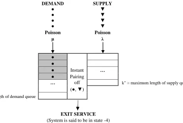
Initially, the authors consider a simple system with only one kind of commodity and many consumers. Both supply and demand are assumed to take place one unit at a time. When there is a demand of one unit, it will be satisfied by commodities in stock, and if there is no item in stock, the demand joins the queue in the demand side and will wait until the commodity becomes available. On the other hand, when the commodity is available and there is no immediate demand for it, it will join the queue on the supply side and will wait until the arrival of the next demand. If a consumer (demand) arrives while k' consumers are already in the queue, it leaves the system. Similarly, when k" units of the commodity (supply) are already in the queue, there will be no more supply to the system. Figure 1 illustrates the model with four demand units waiting for a supply unit to serve.
It will be assumed that units of supply (of commodity, personnel, service, etc.) arrive according to a Poisson process with average rate while units of demand of the same kind arrive according to a Poisson process with average rate . A unit of demand (supply) would be instantly paired off, at time of arrival, with a unit of supply (demand), provided that there is at least one unit of supply (demand) in the system, waiting to be distributed. Otherwise, that unit of demand (supply) would join the queue on the demand (supply) side. The system is said to be in state "-m", m = 0, 1, …, k', if there are m units of excess demand in the queue, and in state "m", m = 1, 2, …, k", if there are m units of excess supply. Both k' and k" are assumed to be finite.
DEMAND SUPPLY
● ▼
● ▼
● ▼
● ▼
Poisson Poisson
μ λ
●
●
● Instant … ● Pairing
… off k" = maximum length of supply queue
(●, ▼)
k' = maximum length of demand queue
3. ANALYTICAL FORMULATION
Strategies to control costs due to imbalance of supply and demand have been considered by Bollapragada and Rao (2006), DeCroix and Arreola-Risa (1998), and Leeman (1964). Mendoza, Sedaghat, and Yoon (2009) considered the effects of managing excess supply. In this paper, the authors focus their attention on situations where demand is higher than supply; that is, when μ > . In these situations, either of two policies may be chosen - reducing the demand, say by increasing the price, or increasing the supply. These two policies and their mathematical formulations are considered next.
3.1 Case I: Balance by Discouraging Demand
Suppose that c' is the cost per time unit of one unit of excess demand in the queue, c" is that of a unit of excess supply in the queue, γ is the demand reduction factor (γ is applied to the given rate μ of demand and the new demand rate becomes γμ, 0 < γ < 1), and cγ is the cost incurred per time unit in reducing the demand rate by one unit. Let Pm be the probability that the system is in state m, where m = -k’,…, 0,…, k". If ρ = /(γμ) denotes the utilization factor, the expected total cost when a demand reduction factor is applied is”
-1 k"
C(γ) = c' Σ (-m) Pm + c" Σ m Pm +cγ μ(1 – γ) (1) m=-k' m=1
where the first summation is the expected undersupply cost, the second is the expected oversupply cost, and the third term is the expected cost of reducing the demand rate from μ to γμ.
The proposed model can be used to find stationary and transient probability distributions. This paper focus on the stationary probabilities of being in a given state after the system is in operation long enough that all influences of the initial states have become negligible. If Pm now denotes the steady-state probability that the system is in state m, where m = -k’,…, 0,…, k", it can be found using balance arguments that the balance equations for steady-state are:
P-k' = γμ P-k'+1
( + γμ) Pm = Pm-1 + γμ Pm+1
Pk"-1 = γμ Pk" (2)
The analytical solution to the above system of linear equations can be obtained based on balance arguments in Markov chains Stewart (1999) and Stewart (1994). If ρ = /(γμ), the solution is given by:
Pm = ρ m + k' (1 - ρ) / (1 - ρ k' + k" +1) if ρ 1 (3)
= 1 / (k' + k" + 1) if ρ = 1. (4)
If the above expressions for Pm are substituted in Equation (1), the expected total cost to the system when a demand reduction factor is applied is given by:
C(γ) = [c' k' (k' + 1) + c" k" (k" + 1)] / [2(k' + k"+ 1)] + cγ μ(1 – γ) if ρ = 1 (5)
= f(ρ) / g(ρ) +cγ μ (1 – γ) if ρ 1 (6)
where:
f(ρ) = - c’ (-k' + ρ + k' ρ – ρ k' + 1) + c”[ ρ k' + 1 - (1 + k") ρ k' + k" + 1 + k" ρ k' + k" + 2 ]
g(ρ) = (1 - ρ) (1 - ρ k' + k" + 1 ) .
3.2 Case II: Balance by Increasing Supply
In this model, the rate of demand μ remains unchanged, but the expansion of supply is replaced by and the last term of Equation (1) is replaced by c (-1). Here, is the supply expansion factor ( > 1) and c denotes the cost incurred per time unit to increase the supply by one. The utilization factor is now ρ = ()/ and the expected cost, when a supply expansion factor is applied, becomes:
-1 k"
C() = c' Σ (-m) Pm + c" Σ m Pm +c ( - 1) (7) m=-k' m=1
The first summation is the expected undersupply cost, the second is the expected oversupply cost, and the third is the expected cost of increasing the supply rate from to .
If Pm now denotes the steady-state probability that the system is in state m, where m = -k’,…, 0,…, k", the balance equations for steady-state are:
P-k' = μ P-k'+1
( + μ) Pm = Pm-1 + μ Pm+1
Pk"-1 = μ Pk" (8)
The solution to Equations (8) with ρ = ()/μ is given by:
Pm = ρ m + k' (1 - ρ) / (1 - ρ k' + k" + 1) if ρ 1 (9)
= 1 / (k' + k" + 1) if ρ = 1. (10)
If the above expressions for Pm are substituted in Equation (7), the expected total cost to the system, when a supply expansion factor is applied, is given by:
C() = [c' k' (k' + 1) + c" k" (k" + 1)] / [2(k' + k"+ 1)] + c ( - 1) if ρ = 1 (11)
= f(ρ) / g(ρ) + c ( - 1) if ρ 1 (12)
where:
f(ρ) = - c’ (-k' + ρ + k' ρ – ρ k' + 1) + c”[ρ k' + 1 - (1 + k") ρ k' + k" + 1 + k" ρ k' + k" + 2]
and
g(ρ) = (1 - ρ) (1 - ρ k' + k" + 1).
4. ANALYTICAL OPTIMAL POLICIES
Table 1: Parameter Values used to Generate 1,440 Scenarios
Parameter Initial Increment Final
k’ 5 10 25
k” 5 10 25
1.00 0.20 1.20
1.20 0.20 2.20
c’ 1.00 0.00 1.00
c” 0.50 0.25 1.25
(*) 0.50 0.25 1.25
(*) c for Case I and cδ for Case II.
The exact values of γ and that minimize such expected total costs were found by iteration using procedure NLP in SAS. Information about procedure NLP can be found visiting the Website http://support.sas.com/rnd/ app/index.html. A discussion and summary of such exact numerical results for Policies I and II are presented below.
4.1 Optimal Solution for Case I
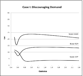
For each scenario, the value of between 0 and 1 that minimizes C() was found. Figure 2 illustrates typical shapes of the relationship between the minimum expected total cost C() and the demand reduction factor . Table 2 specifies the parameter values for the chosen three scenarios of Figure 2. Scenarios 929 and 1440 in Figure 2 correspond to the approximately 93% of instances where C() has two inflection points, its minimum occurs at a value between 0 and 1 and whose value is considerably lower than C(1) where no demand reduction is applied (i.e., = 1). Scenario 337 illustrates the approximately 1% of instances where C() has one inflection point, its minimum occurs at a value of close to 1, and C(1) is barely higher than the minimum.
Table 2: Parameter Values for Figure 2
Scenario # k’ k” c’ c” μ γ Min C(γ)
337 5 25 1 0.50 1.4 1.0 0.8909 3.0290
929 15 25 1 0.50 2.0 1.2 0.6041 7.2790
1440 25 25 1 1.25 2.2 1.2 0.5556 15.3265
4.2 Optimal Solution for Case II
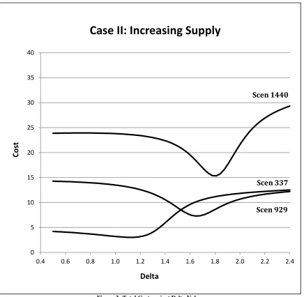
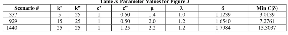
For each scenario, the value of greater than 1 that minimizes C() was found. Figure 3 corresponds to the same scenarios displayed before for Case I (with c instead of c) and illustrates typical shapes of the relationship between the minimum expected total cost C() and the demand expansion factor . Table 3 specifies the parameter values for the chosen three scenarios of Figure 3. Scenarios 929 and 1440 illustrate the approximately 95% of scenarios where C() has two inflection points, the minimum occurs at a value greater than 1. Scenario 337 illustrates instances where C() has a minimum at a value of slightly greater than 1 and where C(1) is barely higher than the minimum.
Figure 3: Total Cost against Delta Values
0 5 10 15 20 25 30 35 40
0.4 0.6 0.8 1.0 1.2 1.4 1.6 1.8 2.0 2.2 2.4
Co
st
Delta
Case II: Increasing Supply
Scen 1440
Scen 337
Table 3: Parameter Values for Figure 3
Scenario # k’ k” c’ c” μ MinC()
337 5 25 1 0.50 1.4 1.0 1.1239 3.0139
929 15 25 1 0.50 2.0 1.2 1.6540 7.2761
1440 25 25 1 1.25 2.2 1.2 1.7984 15.3037
5. APPROXIMATE OPTIMAL POLICIES BY REGRESSION
To determine the model parameters that most affect the optimal γ and , the exact optimal values found for γ and in the previous section were regressed on all model parameters. These fitted regressions may appeal to some practitioners as easy-to-use formulas to get good approximate optimal values for γ and and the corresponding minimum expected total costs. Since the computer simulation leads to computational burden, an analytical approximation solution is sought. To get approximate optimal values for γ and that make the minimum expected total costs, the exact optimal values simulated for γ and in the previous section were regressed on all model parameters.
5.1 Regression Solution for Case I
From the 1,440 original scenarios, 1,401 of them led to feasible solutions that minimized C(γ), including 56 scenarios where γ is greater than 1. Regressions based on these 1,401 scenarios lead to the following best estimate for the optimal γ in terms of the model parameters:
γ-hat = 1.512592 + 0.208415 * (k”/k’) + (-0.0240428) * (k”/k’) 2 + 0.120488 * c” + 0.020565 4* c γ [0.0357] [0.0031] [0.0005] [0.0041] [0.0041]
+ (-1.093527) * (/) + 0.211927 * (/)2 (13)
[0.0424] [0.0125]
It has coefficient of determination R2 = 0.9440 and standard error of estimate se = 0.0421. The figures in square parentheses are the regression coefficients’ standard errors. The regression identifies (k”/k’), (k”/k’)2, c”, c
γ, (/), and (/)2 as the most important regressors in determining the optimal γ. The most significant predictors of the optimal policy are the ratio of the supply queue length over the demand queue length and its square. The next two best predictors are the ratio of the supply rate over the demand rate and its square. The last two best predictors are c”, per time unit of excess supply in the queue, and cγ, the cost incurred per time unit in reducing the demand rate by one. If the parameters of a user lie within the parameter space used to fit the regression (Table 1), the user can use equation (13) to get approximate values of γ and the corresponding expected total cost for the parameter values that he or she has, while the standard errors of the coefficients indicate how sensitive γ-hat is to errors in estimating these regressors. In situations where equation (13) leads to an estimated demand reduction factor greater than 1, use γ-hat = 1.
5.2 Regression Solution for Case II
As in Case I, the exact optimal values found for were regressed on the environmental model parameters. The fitted regression equation allows a user to get approximate values of the optimal and the corresponding expected total cost for the parameter values that he or she has.
-hat = 2.220880 + (-1.985561) * (/)2 + .573832 * (k'/ k") + (-0.273416) * c” + (-.0713564) * c
[0.0249] [0.0198] [0.0162] [0.0100] [0.0100]
+ (-0.061702)* (k'/ k")2 + (-0.100368)* (k”/ k’) + 0.020213 * k” + (-0.013816) * k’ (14) [0.0023] [0.0053] [0.0011] [0.0011]
It has coefficient of determination R2 = 0.9433 and standard error of estimate se = 0.1049. It identifies (/), (k'/ k"), k', k”, and c”, the opportunity cost per time unit of one unit of excess supply in the queue, as the most important factors in determining the optimal . However, c , the cost incurred per time unit to increase the supply by one unit, is not an important factor in predicting the optimal .
If the parameters of a user lie within the parameter space used to fit the regression (Table 1), the user can use (14) to get approximate values of the optimal and the corresponding expected total cost for the parameter values that he or she has. The standard errors of the coefficients indicate how sensitive -hat is to errors in estimating these regressors. In situations where equation (14) leads to an estimated demand expansion factor less than 1, use -hat = 1.
6. AN ILLUSTRATION
A typical case of excess demand is research funding where research proposals compete for scarce funding resources. Research funding is obtained through a competitive process in which potential research proposals are evaluated and only some of the most promising proposals receive funding. An interesting example occurs when researchers request a granting agency to financially support their proposals.
Consider a system where a university/sponsor relationship exists. First, let’s define what sponsorship is. To sponsor something or somebody is to support an event, activity, or organization financially or through the provision of products or services. A sponsor is the individual or group that provides the project funding. When a sponsor is willing to provide sponsorship, it is entered in the supply side of a centralized database. If there are less than k” sponsors in the supply queue, the organization becomes the next candidate for sponsorship. Otherwise, it will remain in the supply side of the university database until there are less than k” sponsors. Assume that the arrival of sponsors into the queue follows a Poisson process with supply rate λ. On the demand side, assume that proposal X needs a sponsor and is entered in the demand side of the database. If there are less than k’ unfilled sponsorship proposals, proposal X joins the demand queue and becomes the next proposal to be potentially sponsored. Otherwise, it will remain in the demand side of the database until there are less than k’ proposals waiting for sponsorship. Eventually, if there is at least one sponsor waiting in the supply queue and no other yet unfunded proposal registered ahead of proposal X, then the first sponsor waiting in the supply queue will sign the sponsorship contract for proposal X. It will be assumed that proposal requests for sponsorship follow a Poisson process with demand rate μ. When there are organizations waiting to offer sponsorship, the supply queue is of positive length. When there are proposals waiting for sponsorship, the demand queue is of positive length.
The models will find the level of demand reduction or supply increase that minimizes the total operational cost of successfully matching one proposal and a donor.
With these parameter values, a non-linear minimization procedure, such as NLP in SAS, can be used to obtain the exact values of γ and that minimize the total cost C(γ) and C(), respectively. Those optimal values are demand reduction factor γ* = 0.6893 with total cost = $9.2698 per day or $3,337 per year and supply expansion factor * = 1.4479 with total cost = $9.2462 per day or $3,329 per year. The total operational costs to successfully match a proposal to a donor are very similar because cγ andcare both equal to 1.25, so the decision on whether to reduce demand or increase supply would be based on other considerations. For instance, what would be preferable - to limit proposals by 31.1% [= (1-0.689310)*100] or to look for additional resources to obtain 44.8% [= (1.447943 – 1)*100] additional donors?
Alternatively, approximate optimal solutions can be found more easily using regression Equations (13) and (14) which lead to the following approximate solutions: Estimated Demand Reduction Factor: γ–hat = 0.709827, estimated total cost = 9.3979 and estimated supply expansion factor –hat = 1.4151, estimated total cost = 9.3256.
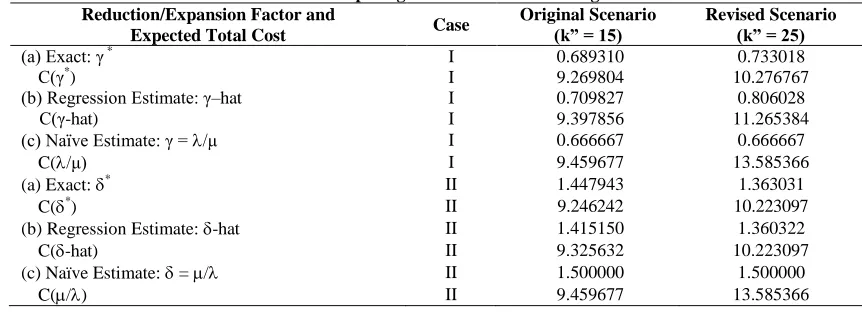
Next, the authors compare the performance of the exact and the regression solutions above with the solutions found ignoring the stochastic nature of the model by setting the utilization factor ρ equal to 1. That is, γ = / for Case I and = μ/ for Case II. Table 4 tabulates results from three strategies - Exact, regression, and non-stochastic. It can be seen that for both policies’ scenarios, regression estimates led to slightly higher minimum costs while the “naïve” solution (found setting ρ equal to one) led to even higher minimum costs.
Since failing to use a willing sponsor is highly undesirable, k” should be chosen large enough to make the chance of such an event, Pk”, rather small. Hence, another potential inquiry that the university is interested in is the effect of increasing the maximum number of sponsors to be pursued from k” = 15 to k” = 25. The last column of Table 4 tabulates the parameter models, the factors and costs for the revised scenario. It can be seen that the minimum cost has to increase to accommodate large donor pool in the revised scenario, but the required reduction and expansion rates are smaller than the original scenario.
Discrepancies of the naïve estimates, with respect to the exact solution, are more noticeable in the revised scenario where k” = 25. The authors recommend using the regression equations only within the parameter space defined in Table 1. Otherwise, γ and should be found by iteration or simulation. In general, results found by setting ρ equal to one are uniformly inferior to regression solutions.
Table 4: Comparing Results for Three Strategies Reduction/Expansion Factor and
Expected Total Cost Case
Original Scenario (k” = 15)
Revised Scenario (k” = 25) (a) Exact: γ *
I 0.689310 0.733018
C(γ*) I 9.269804 10.276767
(b) Regression Estimate: γ–hat I 0.709827 0.806028
C(γ-hat) I 9.397856 11.265384
(c) Naïve Estimate: γ = /μ I 0.666667 0.666667
C(/μ) I 9.459677 13.585366
(a) Exact: * II 1.447943 1.363031
C(*) II 9.246242 10.223097
(b) Regression Estimate: -hat II 1.415150 1.360322
C(-hat) II 9.325632 10.223097
(c) Naïve Estimate: = / II 1.500000 1.500000
C(/) II 9.459677 13.585366
7. CONCLUDING REMARKS
exponentially distributed. Further, supply and demand queues are assumed to have finite maximum lengths k’ and k”, respectively; c’ and c” are variables costs per unit due to a unit of excess of demand and supply, respectively; and cγ and c represent the costs incurred per time unit in reducing the demand rate by one unit or increasing the supply by one unit, respectively. Relying on those assumptions and notations, formulas were derived for the long-run total cost to balance the unbalancing demand and supply as a function of either the demand reduction factor (0 < γ < 1) or the supply expansion factor ( > 1.). These formulas can be used to find, numerically, the policy factors that would minimize the expected total cost to balance the unbalancing queuing system. By comparing the minimum expected total costs, either by increasing supply or by decreasing demand, the best policy is the one leading to the smaller expected total unitary cost.
For the practitioners’ convenience, regression equations were derived to estimate the optimal policy factors based on exact results found in a large number of scenarios. Overall measures of goodness of fit and detailed performance comparisons of representative scenarios indicate that policies based on regression estimates are, in most situations, very close to policies based on exact values and much better than those found setting the utilization factor ρ equal to 1.
It is possible to apply the proposed model to bigger scale situations where fulfillment of demand and supply occur simultaneously; for instance, balancing numbers of sellers and buyers in the stock market, balancing Panama Canal operations between number of waiting ships, and flexible canal capacity. More challenging extensions are the use of more general distributions for the queues or the study of the transient behavior of the system before stationarity is achieved.
ACKNOWLEDGEMENTS
The authors are grateful to Ms. Julija Korsunova for suggesting the Illustration in Section 6.
AUTHOR INFORMATION
Gaston Mendoza holds a Ph. D. in Statistics from Temple University and a MS in Mechanical Engineering from the National Engineering University in Lima, Peru. He recently retired as Associate Professor of Statistics at the Silberman College of Business Administration, Fairleigh Dickinson University. From 1976 to 1982, he headed the Biometrics Unit of the International Center for Tropical Agriculture in Colombia, S. A. His research areas include statistical forecasting and operations research. E-mail: [email protected]
Mohammad Sedaghat is a professor of the Department of Information Systems and Decision Sciences at Fairleigh Dickinson University. He obtained his Ph.D. in Operations Research from Polytechnic University, New York. His research interests include queuing theory and stochastic processes. E-mail: [email protected] (Corresponding author)
K. Paul Yoon is Professor and Chair of Information Systems and Decision Sciences Department at Fairleigh Dickinson University. His M.S. and Ph.D. degrees in Operations Research are from Kansas State University. His research areas include multiple criteria decision-making (MCDM) and its applications to service and production systems. He is the co-author of three books on MCDM. E-mail: [email protected]
Olga Melnyk is a Credit Analyst at Asset Based Lending division of TD Bank. She holds an MBA in Finance and Accounting from Fairleigh Dickinson University. She also holds a MS in Economics and Finance from the Kiev National University of Trade and Economics in Ukraine. E-mail: [email protected]
REFERENCES
1. Bollapragada, R., & Rao, U. S. (2006). Replenishment planning in discrete-time, capacitated, non-stationary, stochastic inventory systems. IIE Transactions, 38(7), 605-615.
3. Brandt, A., & Brandt, M. (2004). On the two-class M/M/1 system under preemptive resume and impatience of the prioritized customers. Queueing Systems, 47, 147-168.
4. Conolly, B. W., Parthasarathyb, P. R., & Selvarajub, N. (2002). N double-ended queues with impatience. Computers & Operations Research, 29, 2053-72.
5. DeCroix, G. A., & Arreola-Risa, A. (1998). On offering economic incentives to backorder. IIE Transactions, 30(8), 715-726.
6. Kashyap, B. R. K. (1996). The double-ended queue with bulk service and limited waiting space. Operations Research, 14, 822-834.
7. Kendall, D. G. (1951). Some problems in the theory of queues. Journal of the Royal Statistical Society, 13(2), 151-85.
8. Kim, W. K., Yoon, K. P., Mendoza, G., & Sedaghat, M. (2010). Simulation model for extended double-ended queuing. Computers and Industrial Engineering, 59(2), 209-219.
9. Leeman, W. (1964). The reduction of queues through the use of price. Operations Research, 12, 783-85. 10. Mendoza, G., Sedaghat M., & Yoon, K. P. (2009). Queuing models to balance systems with excess supply.
International Journal of Business & Economics Research, 8(1),91-103.
11. Parra, I., & Gallego, J. A. (1999). Multiproduct monopoly: A queueing approach. Applied Economics, 31(5), 165-176.
12. Perry, A., & Stadje, W. (1999). Perishable inventory systems with impatient demands. Mathematical Methods in Operations Research, 50, 77-90.
13. Sasieni, M. W. (1961). Double queues and impatient customers with applications to inventory theory. Operations Research, 9,771-81.
14. Stewart, W. J. (1999). The numerical solution of Markov chains. New York: Marcel Dekker.
15. Stewart, W. J. (1994). An introduction to the numerical solution of Markov chains. NJ: Princeton University Press.