Robot Motion Planning Under Topological Constraints

University of Pennsylvania

ScholarlyCommons

Publicly Accessible Penn Dissertations

1-1-2013

Robot Motion Planning Under Topological

Constraints

Soonkyum Kim

University of Pennsylvania, [email protected]

Follow this and additional works at:

http://repository.upenn.edu/edissertations

Part of the

Mechanical Engineering Commons

, and the

Robotics Commons

This paper is posted at ScholarlyCommons.http://repository.upenn.edu/edissertations/883 For more information, please [email protected].

Recommended Citation

Kim, Soonkyum, "Robot Motion Planning Under Topological Constraints" (2013).Publicly Accessible Penn Dissertations. 883.

Robot Motion Planning Under Topological Constraints

Abstract

My thesis addresses the the problem of manipulation using multiple robots with cables. I study how robots

with cables can tow objects in the plane, on the ground and on water, and how they can carry suspended

payloads in the air. Specifically, I focus on planning optimal trajectories for robots.

Path planning or trajectory generation for robotic systems is an active area of research in robotics. Many

algorithms have been developed to generate path or trajectory for different robotic systems. One can classify

planning algorithms into two broad categories. The first one is graph-search based motion planning over

discretized configuration spaces. These algorithms are complete and quite efficient for finding optimal paths in

cluttered 2-D and 3-D environments and are widely used [48]. The other class of algorithms are optimal

control based methods. In most cases, the optimal control problem to generate optimal trajectories can be

framed as a nonlinear and non convex optimization problem which is hard to solve. Recent work has

attempted to overcome these shortcomings [68]. Advances in computational power and more sophisticated

optimization algorithms have allowed us to solve more complex problems faster. However, our main interest is

incorporating topological constraints. Topological constraints naturally arise when cables are used to wrap

around objects. They are also important when robots have to move one way around the obstacles rather than

the other way around. Thus I consider the optimal trajectory generation problem under topological

constraints, and pursue problems that can be solved in finite-time, guaranteeing global optimal solutions.

In my thesis, I first consider the problem of planning optimal trajectories around obstacles using optimal

control methodologies. I then present the mathematical framework and algorithms for multi-robot

topological exploration of unknown environments in which the main goal is to identify the different

topological classes of paths. Finally, I address the manipulation and transportation of multiple objects with

cables. Here I consider teams of two or three ground robots towing objects on the ground, two or three aerial

robots carrying a suspended payload, and two boats towing a boom with applications to oil skimming and

clean up. In all these problems, it is important to consider the topological constraints on the cable

configurations as well as those on the paths of robot. I present solutions to the trajectory generation problem

for all of these problems.

Degree Type

Dissertation

Degree Name

Doctor of Philosophy (PhD)

Graduate Group

Mechanical Engineering & Applied Mechanics

First Advisor

Keywords

Motion Planning, Robot, Topology

Subject Categories

ROBOT MOTION PLANNING UNDER TOPOLOGICAL CONSTRAINTS

Soonkyum Kim

A DISSERTATION

in

Mechanical Engineering and Applied Mechanics

Presented to the Faculties of the University of Pennsylvania

in

Partial Fulfillment of the Requirements for the

Degree of Doctor of Philosophy

2013

Supervisor of Dissertation

Vijay Kumar, Professor

Department of Mechanical Engineering and Applied Mechanics

Graduate Group Chairperson

Prashant K. Purohit, Associate Professor

Department of Mechanical Engineering and Applied Mechanics Dissertation Committee

Mark Yim, Professor, Department of Mechanical Engineering and Applied Mechanics Vijay Kumar, Professor, Department of Mechanical Engineering and Applied Mechanics Robert Ghrist, Professor, Department of Mathematics

ROBOT MOTION PLANNING UNDER TOPOLOGICAL CONSTRAINTS

COPYRIGHT

2013

Soonkyum Kim

This work is licensed under the Creative Commons

Attribution-NonCommercial-ShareAlike 3.0 License.

Acknowledgments

First, I would like to express my sincere gratitude toward my advisor, Prof. Vijay Kumar for his ceaseless, dedicated and invaluable advise and guidance during the course of my graduate studies at GRASP Laboritory in the University of Pennsylvania. I would also like to heartily thank Prof. Mark Yim and Prof. Maxim Likhachev for their valuable time and effort in serving as my dissertation committee members. I also like to thank Prof. Robert Ghrist, not only for being on my dissertation committee, but also for collaborating on the topological exploration problem. I would also like to thank Dr. Subhrajit Bhattacharya for valuable discussions and for collaborating on many of the problems presented in this thesis. I would like to express my gratitude toward Prof. Frank C. Park who introduced me to the field of robotics.

My sincere appreciation goes to Dr. Koushil Sreenath for his collaboration on the problem of optimal trajectory generation under topological constraints. I would also like to thank Dr. Nathan Michael for collab-orating on the aerial manipulation problem, and Dr. Peng Cheng for collabcollab-orating on the cooperative towing problem. My sincere thanks goes to Dr. Jornathan Fink for his collaboration on both the aforesaid problems. I would like to thank Prof. Gaurav Sukhatme and Hordur Heidarsson of USC for their collaboration on the field experiments in the problem related to manipulation of a set of objects.

ABSTRACT

ROBOT MOTION PLANNING UNDER TOPOLOGICAL CONSTRAINTS

Soonkyum Kim

Vijay Kumar

My thesis addresses the the problem of manipulation using multiple robots with cables. I study how robots with cables can tow objects in the plane, on the ground and on water, and how they can carry sus-pended payloads in the air. Specifically, I focus on planning optimal trajectories for robots.

Path planning or trajectory generation for robotic systems is an active area of research in robotics. Many algorithms have been developed to generate path or trajectory for different robotic systems. One can classify planning algorithms into two broad categories. The first one is graph-search based motion planning over discretized configuration spaces. These algorithms are complete and quite efficient for finding optimal paths in cluttered 2-D and 3-D environments and are widely used [48]. The other class of algorithms are optimal control based methods. In most cases, the optimal control problem to generate optimal trajectories can be framed as a nonlinear and non convex optimization problem which is hard to solve. Recent work has attempted to overcome these shortcomings [68]. Advances in computational power and more sophisticated optimization algorithms have allowed us to solve more complex problems faster. However, our main interest is incorporating topological constraints. Topological constraints naturally arise when cables are used to wrap around objects. They are also important when robots have to move one way around the obstacles rather than the other way around. Thus I consider the optimal trajectory generation problem under topological constraints, and pursue problems that can be solved in finite-time, guaranteeing global optimal solutions.

Contents

1 Introduction 1

1.1 Introduction . . . 1

1.2 Literature review . . . 2

1.3 Contribution . . . 4

2 Preliminaries 5 2.1 Curves in(W− O) . . . 5

2.2 Homology and Homotopy Invariants . . . 5

2.2.1 Homology of curves and Homology Invariants . . . 5

2.2.2 Homotopy of curves and Homotopy Invariants . . . 7

2.2.3 The Hurewicz map . . . 9

2.2.4 Augmented Graph . . . 10

3 Trajectory Generation under Topological Constraints 12 3.1 Optimal Trajectory Generation . . . 12

3.2 Optimal Trajectory with Homology Class Constraints . . . 15

3.2.1 Algorithm Description . . . 15

3.2.2 Simulation Results . . . 21

3.3 Optimal Trajectory with Homotopy Class Constraints . . . 24

3.3.1 Algorithm Description . . . 24

3.3.2 Simulation Results . . . 26

3.4 Conclusion . . . 27

4 Topological Exploration 29 4.1 Motivation . . . 29

4.2 The Quotient Space andH-signature . . . 30

4.3 The Algorithm . . . 32

4.3.1 Representation . . . 32

4.3.2 Multi-robot Exploration Algorithm . . . 32

4.3.3 Distributed Implementation . . . 37

4.4 Results . . . 37

4.4.1 Partially Known Environment . . . 37

4.4.3 Experiment with a Single Robot . . . 39

4.5 Conclusion . . . 39

5 Manipulation with Cables 42 5.1 Cooperative Towing With Multiple Ground Robots . . . 42

5.1.1 The Quasi-Static Model for Cooperative Towing . . . 42

5.1.2 Equilibrium Analysis . . . 45

5.2 Kinematics and Statics of Cooperative Multi-Robot Aerial Manipulation with Cables . . . . 48

5.2.1 Kinematics of Planar Manipulation Systems . . . 48

5.2.2 Direct Problem . . . 50

5.2.3 Direct problem:n=2 . . . 50

5.2.4 Direct problem:n=3 . . . 52

5.2.5 Stability . . . 54

5.3 Conclusion . . . 55

6 Manipulation of A Set Of Objects 57 6.1 Introduction . . . 57

6.2 Problem Description . . . 59

6.3 Separating Configurations . . . 61

6.4 Implementation . . . 64

6.4.1 Planning in Joint State-space . . . 64

6.4.2 Decoupled Planning: A Distributed Approach . . . 65

6.4.3 Sequential Planning . . . 67

6.5 Result . . . 69

6.5.1 Simulation Results . . . 69

6.5.2 Dynamic Simulation and Fast Re-planning . . . 71

6.5.3 Experiment Results . . . 78

6.6 Sequential Manipulation of Large Number of Objects . . . 79

6.6.1 Algorithm . . . 80

6.6.2 Simulation Result . . . 82

6.7 Conclusion . . . 83

7 Conclusion 84 7.1 Summary . . . 84

7.2 Main Contributions . . . 84

7.3 Future Work . . . 85

A Heuristic distance function considering the homotopy class constraints 88 A.1 Algorithm . . . 88

List of Figures

2.1 Illustration of homology class and homotopy class or curves. . . 6

2.2 Examples of possibleH-signature functions. . . 7

2.3 Examples of homotopy class invariant function on2-dimensional plane. . . 8

2.4 Examples where curves (τ1andτ2) are homologous, but not homotopic. . . 9

2.5 Example of augmented graph. The goal vertices of two different paths,τ1andτ2, have the same coordinates but considerd to be different vertex in the augmented graph. . . 11

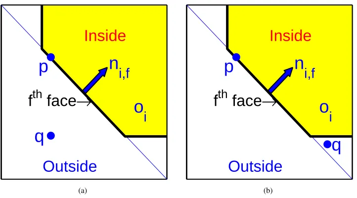
3.1 The normal vector,ni,f, of thefthface of obstacleoi is pointing inward. pis an arbitrary point on thefthface. (a) An example ofq ∈Qwhenbi,f = 0. (b) An example ofq ∈Q whenbi,f = 1. . . 13

3.2 (a) Overlapping subsets divided by values of binary variables representing each face of tri-angular obstacle. (b) Disjointed cells divided by values of binary variables representing each face but considering additional constraint. . . 13

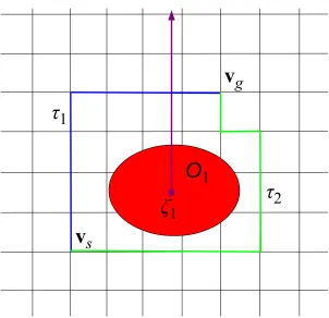
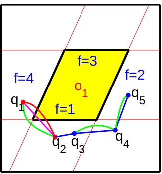
3.3 An example of parallelogram obstacle.fis the index of each face. Red and magenta curves are infeasible trajectories between two feasible configurations,q1andq2. Adjacent interme-diate points(q3,q4andq5) are satisfying additional constraint. . . 16

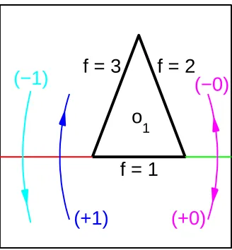
3.4 An example of calculating the h-signature with respect to a triangular obstacle. . . 18

3.5 Starting from a piece-wise linear curve (cyan), we can progressively add points, to make the trajectory smoother by increasing the order of differentiability by one at each step. . . 20

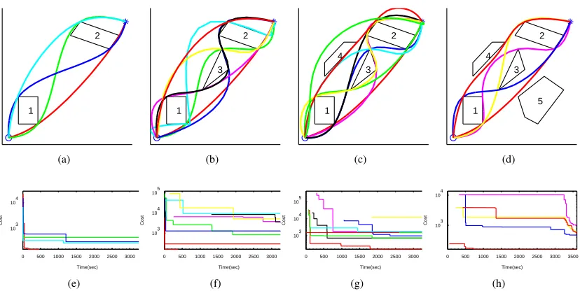
3.6 Simulation result of trajectory generation in four different homology classes with the same initial configuration (left bottom point) and final configurations(right upper point). The first obstacle is parallelogram and the second obstacle is triangle. The actual compu-tation time(sec) and optimal costs are specified on the upper left corners of plots. (a) Hd= [−1,−1]T. (b)Hd= [−1,0]T. (c)Hd= [0,−1]T. (d)Hd = [0,0]T. . . 22

3.7 Simulation result with anytime solutions. The computation time(sec)and optimal costs are specified on the upper left corners of each plot. . . 22

3.8 (a)-(d) Final trajectories in four different homology classes with two, three, four and five obstacles, respectively. (e)-(h) Cost of the trajectories along with computation time with two, three, four and five obstacles, respectively. The plots shows the change in cost with time plotted in log scale. . . 23

3.10 (a) Optimal trajectory without homotopy constraints (b)-(e) Trajectories with four different homotopy class constraints. The thick black curve is the optimal trajectory in each homotopy class and thin gray curves are the suboptimal trajectories for each word. The cost (J) for each case is specified on the upper left corners of plots. . . 26 3.11 (a)-(e) Effect of varying the time distribution in each cell through iterations of the

opti-mization (3.3.2). The number of iterations (itr) and cost are also specified on the upper left corner of each plot. Note that the cost converges to the local optimal cost of the case of Figure 3.10(b) in 6 iterations. . . 27 4.1 Partially explored environments. The group of robots (red dots) need to be split and deployed

for exploration of the unknown regions (pale yellow region marked asL). The figures illus-trate the distinction between frontier-based and topology-based deployments. . . 31 4.2 A simple illustration of a quotient map. The setLis collapsed to a point,q(L). Here we

consider the Euclidean plane,R2, with its subsetLbeing the entire region outside a small

disk on the plane. CollapsingLto a single point gives us the topological2-sphere. All non-trivial1-cycles (or closed loops) that completely lie inLbecome trivial in the quotient space under the quotient map,q. . . 31 4.3 Illustration of algorithmToplogicalExplore. . . 33 4.4 Comparison between the frontier-based exploration algorithm (top row) of [100] and our

T opologicalExplore algorithm (bottom row) in a partially-known environment using 4

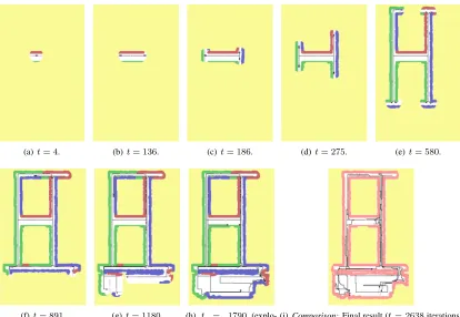
robots. The purple curves show parts of the planned paths, while black represents traversed paths. White is known/explored, while light yellow is the unknown region. . . 38 4.5 The SCARABmobile robot platform [65] . . . 39 4.6 (a)-(h): Simulation result with8 robots exploring an indoor office-like environment. (i):

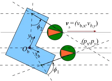
Comparison of performance with frontier-based algorithm of [100] (in the same environ-ment, with same number of robots and same initial configurations). . . 40 4.7 Experiment result with a single robot exploring an indoor office-like environment. . . 40 5.1 Quasi-static manipulation: The object is supported by three support points,Si, with normal

forces (out of the plane),λn,iand tangential frictional forces,λt,i. It is pulled bymcables,

each exerting a forceλc,j. Note the robotRj pulls by moving the object with a prescribed

(given) velocity,VRj. . . 43

5.2 (Left) Arbitrary initial configuration. (Right) Stable equilibrium configuration. (This figure is taken from [24].) . . . 45 5.3 The equilibrium of two-robot towing. (This figure is taken from [24] and reproduced.) . . . 47 5.4 The planar system modeled as a four-bar-linkage. The suspended payload is the coupler with

an assumed center of mass at the middle point of the coupler. . . 49 5.5 A graphical depiction of the conditions presented in Proposition 5.2.2. (This figure is taken

from [40].) . . . 52 5.6 A coupler curve with twelve equilibrium configurations. The stable and unstable

5.7 The six equilibrium configurations of Figure 5.6. Clearly Figures. 5.7(a)-5.7(c) are infeasible when considering tension constraints. . . 56 6.1 The problem of separating the two types of objects. . . 58 6.2 An example of separating configuration and a set of paths to the separating configuration. . . 58 6.3 The solutions of object separating problem is not unique. . . 59 6.4 An example of separating configurations achieve by intuition when considering point objects. 61 6.5 An example of separating configurations which requires smart controller for transporting. . . 61 6.6 Examples of separating configurations which do not satisfy Proposition 6.3.1. . . 63 6.7 Illustration for Proof of Proposition 6.3.2. . . 63 6.8 The environment and its discretization. . . 64 6.9 Decoupled and distributed planning: Optimal paths with differenth-signatures found for the

two robots in parallel threads, and costs of compatible pairs are compared to find the optimal compatible pair. . . 66 6.10 An example of heuristic cost(the sum of the length of green lines) of the path start from

the green circle to the boundary while the desired homotopy class ishd =“r+2r +

3”. In this

example, we ignore the feasibility of the path with respect to objects. . . 68 6.11 A simple30×30environment withr = b = 3. The green & yellow are the paths of the

robots. The rays emanating fromζj are also shown. The dark gray segment indicates the

initial cable configuration. . . 70 6.12 Decoupled, distributed plans. Initial cable is shown in gray/black. Paths are in green and

yellow. . . 70 6.13 Sequential plan. Initial cable is shown in gray/black. Paths are in green and yellow. . . 71 6.14 The dynamic model showing a discrete model of the cable consisting ofnrigid segments

and two rigid circular objects. . . 72 6.15 The three types of contacts considered in the model. . . 74 6.16 When the center of an object lies in the yellow region, we need to check for contact between

theith_{segment of the cable and the object. The boundary of yellow region (i.e. the green}

lines) are perpendicular to(wi −wi−1). In this example, we need to check for contact

betweenith_{segment ando}

1, but noto2. . . 75

6.17 Dynamic simulation for separation of objects. The gray curve is the cable, with black dots marking robots at its ends. Green curves are the planned paths. Magenta curves are the robot footprints. Red & blue disks are the rigid freely-floating objects. See http://youtu.be/GyCn-8yDzO0 for video. . . 78 6.18 Experiments with Autonomous Boats conducted by H. K. Heidarsson, University of

South-ern California [56]. Red and blue circles are Buoys (objects). Thin gray curve is the planned paths of two ASVs. The Black curve is the current cable configuration. See http://youtu.be/vGgca2w2UdA for video. . . 78 6.19 A large problem. Red and blue dots are object. Green curves are cable-robot teams. Light

6.20 An example of coarse grid. the given workspace is split into set of cells whose boundaries are the reference rays, the cyan lines, and the grey lines. the topology class of path does not change when crossing the grey lines. . . 81 6.21 Dynamic simulation for separation of a large number of objects with multiple cable-robot

teams via sequential manipulation. The red and blue dots are the objects. The green curves are the cables. The red and blue t’s are the baskets. Yellow boxes are the workspace of each cable-robot team. Magenta curves are the paths of the robots. See http://youtu.be/ZHrEIo8dGDA for video. . . 83 A.1 The cost ofch

pr(qi, rsk)is sum of the length of green lines. This Figure illustrate the case

Chapter 1

Introduction

1.1

Introduction

Path planning or trajectory generation for robotic systems is an active area of research in robotics. Many algorithms have been developed to generate path or trajectory for different robotic systems. One can classify planning algorithms into two broad categories. The first one is graph-search based motion planning over discretized configuration spaces. These algorithms are complete and quite efficient for finding optimal paths in cluttered 2-D and 3-D environments and are widely used [48]. The other class of algorithms are optimal control based methods. In most cases, the optimal control problem to generate optimal trajectories can be framed as a nonlinear and non convex optimization problem which is hard to solve. Recent work has attempted to overcome these shortcomings [68]. Advances in computational power and more sophisticated optimization algorithms have allowed us to solve more complex problems faster. However, our main interest is incorporating topological constraints. Topological constraints naturally arise when cables are used to wrap around objects. They are also important when robots have to move one way around the obstacles rather than the other way around. Thus I consider the optimal trajectory generation problem under topological constraints, and pursue problems that can be solved in finite-time, guaranteeing global optimal solutions.

Early works on path planning or trajectory generation problem discussed the algorithms for mobile robots on the plane. Time optimal trajectories of differential drive mobile robots, which can rotate in position, can be computed by following sequence of primitive motions of rotating in position and straight moves [5]. If the vehicle has minimum turning radius, then the shortest path will consist of a sequence of arcs and straight lines [79]. Also, in [37] the authors find smooth shortest path with restriction on average curvature. Elastic bands introduced the algorithm to deform the path mobile robots in dynamic environments [78], which has been extended to mobile manipulation problem [22, 103]. Of course, finding smooth optimal trajectory is still one of active research topic. Recently, such problem has been extended to 3D path planning of UAVs [64].

distinguish the class of paths or trajectories. Also, we want to find optimal paths or trajectories indifferent

classes.

Cables are widely used in mechanical systems to transfer actuator powers. However, humans utilize cables or ropes to carry or manipulate various objects and there has been active research on utilizing cables in robot planning and control. We can transport a payload by towing with cables. Usually, this method requires one or multiple robot to carry a single payload. We can manipulate a larger number of small objects by skimming via cable. For efficiently manipulate objects, it is necessary to consider the configuration of the cable in planning and control.

The topology can give us the answer of these problem. The paths or trajectories are different if they are in different topology classes. Also, the objects separation problem can be formulated to path planning problem with topological constraints of the cable configuration and robot paths.

In my thesis, I first consider the problem of planning optimal trajectories around obstacles using optimal control methodologies. I then present the mathematical framework and algorithms for multi-robot topolog-ical exploration of unknown environments in which the main goal is to identify the different topologtopolog-ical classes of paths. Finally, I address the manipulation and transportation of multiple objects with cables. Here I consider teams of two or three ground robots towing objects on the ground, two or three aerial robots car-rying a suspended payload, and two boats towing a boom with applications to oil skimming and clean up. I present solutions to the trajectory generation problem for all of these problems.

1.2

Literature review

Trajectory generation problem for robotic systems is one of the most active areas in robotics research. Some literatures focus on finding optimal trajectories in convex or unbounded spaces [6, 19]. However, the de-velopment of computational capacities allows algorithms for generating trajectories in cluttered, non-convex environments with kinematic and dynamic constraints in the form of constraints on communication, cov-erage, environment, time, etc (see kinodynamic planners [35], RRT trees [61], LQR trees [94], Elastic Roadmaps [103] and references within). Most of the algorithms are developed to find optimal trajectories satisfying feasibility constraints. However, there have also been considerable amount of research interest in algorithms for generating trajectories for multi-agent problems [47, 28, 105]. In such problems it is often required that each robot follows different trajectories to cover or sense the whole work space as in search-and-rescue or surveillance problems. This brings forth the necessity of finding trajectories in topologically different classes. This requires that we impose constraints on the homotopy classes of the trajectories accord-ingly. However, in many practical robotic problems, homology class constraints act a suitable and convenient substitute for homotopy class constraints [14].

Exploration and mapping have been treated quite extensively in the robotics literature. The general problem can be formulated as finding the next best view or pose [77] to acquire information required to build a map of the environment [88]. In most settings, the spatial representation of the map is based on metric information. Indeed approaches like metric-based multi-robot coordinated exploration have been studied widely in the past [11, 17, 87]. In decision-theoretic approaches to exploration, mutual information and entropy are often used [87, 89, 85, 95] to guide robots to perform efficient exploration. Simpler approaches involving the identification of frontiers and segmentation representing the boundaries between unexplored and explored regions have also been widely used for deployment of robots in exploration and mapping of unknown or partially known environments [102, 41, 100].

The advantages of using ropes with robots for manipulation were demonstrated by Donaldet al[34]. An interesting problem that arises in these settings is the modeling of the shape of the cable and the motion planning for the robots to control the position and shape of the cable. Motion planning for manipulation of rope-like flexible objects is discussed in [82]. The problem of entangling and disentangling knots and the motion planning for this problem has been addressed in [60].

From the standpoint of robotics, towing is an important manipulation process [63]. The kinematics and dynamics of cable-actuated, parallel manipulators, which have been studied extensively [75, 20, 92, 99]. However, this body of literature primarily addresses the control of the cable extensions or forces in order to manipulate the payload. In contrast, towing involves cables of fixed length where manipulation is accom-plished by controlling the motions of the ”pivot points” in the parallel manipulators. While manipulation using cables has been studied in the context of distributed manipulation [33, 31, 32], these papers do not address the mechanics or control of the cooperative manipulation task.

The use of robots to tow objects using cables is discussed in [53, 23]. In [23], Chenget alestablish the quasi-static towing problem withncables has a unique solution under certain conditions. In other words, if the robot motions are known, there is instantaneously a unique object motion. An extension of these ideas leads to using a cable with its ends tied to robots to cage and tow objects. Indeed this method is widely used in skimming operations on water surfaces [81, 54]. A description of the dynamics of such systems and an analysis of the problem of cooperative skimming are provided in [12, 4]. However, this work does not explicitly address the manipulation of objects.

In [66], manipulation and transportation with three aerial robots permits full six-dimensional pose con-trol of a cable-actuated payload in three-dimensions despite the fact that the system is underactuated and limited by unilateral tension constraints for specific robots-cables-platform configurations. Aerial towing, the manipulation of a payload suspended by a cable from a moving aerial robot, has been studied in [70]. It is quite clear that the control of all six degrees of freedom requires more than one aerial robot and multiple cables. The underlying mechanics in such systems is closely related to the mechanics of cable-actuated par-allel manipulators in three dimensions. In both cases, the position and orientation of the suspended payload can only be obtained by solving the kinematic equations and the equations of static equilibrium. The equi-librium solutions are configurations in which the gravity wrench is equilibrated by the wrenches exerted by thencables. This means that the lines of action of thencables can only belong to certain subspaces which are linear complexes (forn= 5), linear congruences (forn= 4) or reguli (forn= 3) [51, 76]. Forn <3, it is not possible to achieve an arbitrary position and orientation.

control is accomplished by varying the lengths of multiple cable attachments. These systems offer similar workspace [92, 99], control [73, 74], and analysis [20].

The problem of finding a hypersurface separating two types of objects is studied as part of statistical classification problems [18, 93]. However such methods are susceptible to finding curves that can have disjoint components, do not have guarantees on optimality, and are statistical in nature.

1.3

Contribution

The first contribution of this thesis is generating an optimal trajectory that minimizes an integral cost func-tional (which depends on the trajectory), while also respecting kinematic constraints of the system, avoiding obstacles, and constraining the trajectory to a particular topology class. Although several of these subprob-lems have been solved separately (see [35, 61, 94, 97, 13, 14]), there is no literature, to our knowledge, that addresses the combined problem described above. We suggest the trajectory generation problem under topology class constraints which can be formulated as a MIQP or QP. This method can be used for trajectory generation for differentially-flat systems [72] with a two-dimensional flat output space, such as a kinematic car [71], or a tricycle robot [7], which not only produces a trajectory respecting the homology constraint, but also provides the nominal feedforward forces (due to the differential-flatness property,) for use in feedback control for trajectory tracking.

The second contribution of this thesis is to present the mathematical framework and algorithms for multi-robot topological exploration of unknown environments in which the main goal is to identify the different topological classes of paths. We consider two-dimensional configuration spaces. At any point in time, the robot’s map consists of known, partially-mapped obstacles. The unknown, yet-to-be-explored area is mapped to a single point, thus giving us a quotient space. The topological classes on the quotient space allows us to define topological classes of paths connecting a robot pose to the unknown region in the original configuration space. Robots explore this configuration space choosing different homology classes when confronted by obstacles or walls.

Chapter 2

Preliminaries

In this chapter, we will briefly review topology of paths/trajectories of robots and cables, which can be considered as a curve in the workspace.

2.1

Curves in

(

W

− O

)

LetW ⊂R2be a2-dimensional simply connected and bounded region. Suppose it contains a set of objects, O=O1∪O2∪ · · · ∪On ⊆ W, whereO1, O2,· · · , Onarencounts of objects. Each object,Ojis assumed

to be connected.

Both robot paths/trajectories and cable configurations are1-dimensional curves in(W− O). They can thus be defined as continuous maps from the line segment[0,1]to(W − O). We say a curve,γ: [0,1]→

(W− O), is embedded [69] ifγ(t)6=γ(t0),∀t6=t0(i.e.the curve does not intersect itself).

For a given curve,γ, we define−γ : t 7→ γ(1−t). That is, −γ is the same curve as γ, but with opposite orientation. The line integral of a differential 1-form, ω = f dx+g dy, overγ is defined as

R γω:=

R1

0 (fγ˙x+gγ˙y) dt.

2.2

Homology and Homotopy Invariants

2.2.1

Homology of curves and Homology Invariants

Definition 2.2.1 (Homology classes of curves). Two curves γ1, γ2 : [0,1] → (W − O) connecting the

same start and end points, are homologous (or belong to the samehomology class) iffγ1together withγ2

(the latter with opposite orientation) forms the complete boundary of a2-dimensional manifold embedded in(W − O)(not containing/intersecting any of the objects/obstacles) as shown in Figure 2.1(a) [15, 49].

Ahomology invariantis a function,H, from the space of all curves in(W− O)(with fixed end points) to another much smaller space (in this case, a vector space), such thatH(γ1) =H(γ2)iffγ1is homologous

x

x

O

O

τ

τ

τ

-τ

O

A

-τ

(a) τ1is homologous toτ2 sinceτ1 t −τ2 formsA, the

complete boundary of a2-dimensional manifold embedded in(W− O).τ3belongs to a different homology class since

τ1t −τ3orτ2t −τ3enclosesO2.

x

x

O

O

τ

τ

τ

O

(b) τ1 is homotopic toτ2 since there is a continuous

se-quence of trajectories representing deformation of one into the other. τ3belongs to a different homotopy class since it

cannot be continuously deformed into any of the other two.

Figure 2.1: Illustration of homology class and homotopy class or curves. results from complex analysis. In particular,

H(γ) = 1 2πi Z γ        1

z−ζ1,

1

z−ζ2,

.. .

1

z−ζn

      

dz (2.2.1)

where,z=x+iyis the complex representation of(x, y)∈W − O, andζj =ζj,x+iζj,yare the complex

representations ofrepresentative pointsinside the objects with respect to which we compute theH-signature ans shown in Figure 2.2(a). Thus, the function,H, is computed as the integration of the vector of differential

1-forms,

ωj= 1 2πi

dz z−ζj

, (2.2.2)

over the curveγ.

However, the possible choice of such invariants has been broadened in [16], where the choice of the vector of differential1-forms, which needs to be integrated overγto obtain the invariant, has been proven to be any complete set of generators of thede Rham cohomology group,H_dR1 (W− O). In particular, thebump 1-forms[21],

ωj =υ(y−ζj,y)δ(x−ζj,x)dx, (2.2.3)

(whereδis theDirac delta function, and its integral,υ, is theheaviside step function– that is, informally speaking,ωjare analogous to aDirac deltadistribution over rays emanating fromζjalong positiveY axis)

x

x

O

ζ

γ

ζ

ζ

ζ

ζ

O

O

O

O

(a)H-signature based on simple results from complex anal-ysis.

x

x

O

ζ

γ

ζ

ζ

ζ

ζ

O

O

O

O

X

Y

(b)H-signature based onbump1-forms.

Figure 2.2: Examples of possibleH-signature functions. emanating fromζj (Figure 2.2(b)). In particular, define,#jγ :=

R

γωj =(Number of timesγcrosses the

ray emanating fromζjfrom left to right)−(Number of timesγcrosses the ray emanating fromζjfrom right

to left). Then,

H(γ) =      

#1γ,

#2γ,

.. ., #nγ       . (2.2.4)

For example, curveγin Figure 2.2(b) has theH-signature ofH(γ) = [0,1,0,−1,0]T_{. For closed loops}

the value of H-signature won’t depend on the choice of the differential1-forms, as long as they form a generating set of the firstde Rham cohomology group,H1

dR(W − O)[21], and will compute thewinding numbersaboutζj.

And we can find more generalized form of theH-signature of the given curve,γ: [0,1]→(W − O), with arbitrary reference lines.

#jγ= Z 1

0

υ(dj·(γ(t)−ζj))δ(d˜j·(γ(t)−ζj))dt (2.2.5)

wheredj= [dj,x, dj,y] T

is the direction of the reference line andd˜j= [dj,y,−dj,x] T

is the normal vector to the reference line. So, it is obvious that (2.2.3) is a special case ofdj= [dj,x, dj,y]T = [0,1]T. As a result,

we can choose arbitrary reference lines to calculateH-signature of the given curves and environments.

2.2.2

Homotopy of curves and Homotopy Invariants

Definition 2.2.2(Homotopy classes of curves). Two curvesγ1, γ2: [0,1]→(W− O)connecting the same

x

x

O

ζ

γ

ζ

ζ

ζ

ζ

O

O

O

O

ζ

O

r

r

r

r

r

r

(a) h-signature based on reference rays. h(γ) = “r+₁r+₂r₃+r−₂r−₅”.

x

x

O

ζ

γ

ζ

ζ

ζ

ζ

O

O

O

O

ζ

O

r

r

r

r

r

r

η

(b) h-signature of a closed loop. h(γ t −η) = “r+₂r+₃r₂−r+₆”.

Figure 2.3: Examples of homotopy class invariant function on2-dimensional plane. deformed into the other without intersecting any obstacle as sown in Figure 2.3(a).

Formally, ifγ1 : [0,1] → (W − O)andγ2 : [0,1]→ (W − O)represent the two trajectories (with γ1(0) =γ2(0) =xsandγ1(1) =γ2(1) =xg), thenγ1is homotopic toγ2iff there exists a continuous map η : [0,1]×[0,1]→ (W − O)such thatη(α,0) =γ1(α)∀α∈[0,1], η(β,1) =γ2(β)∀β ∈[0,1], and η(0, γ) =xs, η(1, µ) =xs∀µ∈[0,1][15, 49].

Homotopy invariants, in general, are much more difficult to design and compute. Homotopy groups, unlikehomology groups, do not have the natural structure of a vector space [49]. However, for curves in

2-dimensional plane with punctures (i.e.obstacles/objects), there is a relatively simple representation of the homotopy group and a way of computing the homotopy class of a given curve [46, 50, 98, 49, 9]: We con-siderrepresentative points,ζias before, andparallel non-intersectingrays,r1, r2,· · ·, rn, emanating from

the objects respectively (Figure 2.3(a)). We form awordby tracingγ, and consecutively placing the letters of the rays that it crosses, with a superscript of ‘+1’ (assumed implicitly) if the crossing is from left to right, and ‘−1’ if the crossing is from right to left. Thus, for example, the word forγin Figure 2.3(a) will be “r+₁r+₂r+₃r₂−r+₆r₆−r₅−”. We canreducethis word by canceling the same letters that appear consecutively but with opposite superscript signs. Thus, the word forγ in Figure 2.3(a) can be reduced to “r₁+r+₂r+₃r−₂r−₅”. This reduced word representation is ahomotopy invariantfor open curves (with fixed end points),γ, and we will write this ash(γ)and call it the “h-signature ofγ”. However, it is important to note that we cannot ex-change position for arbitrary pairs of letters in the word (i.e.the juxtaposition of letters isnon-commutative). Unlike thehomology invariant, this is not a vector, but an element of thenon-abeliangroupfreely generated

[86, 49] by{r1, r2,· · · , rn}. Thus, althoughwordscan’t be added in the sense of vectors, they can be

con-catenated under the non-commutativegroup operation, ‘’. Also, the inverse of a word,w, written asw−1, is theh-signature of the same curve but with opposite orientation (i.e. h(−γ) = (h(γ))−1), and is a word where the order of the letters are reversed, and the exponent of each letter is flipped (so thatww−1=“ ”, the identity element). Thus,(w1w2)

−1

=w2−1w1−1. As an example,(“r1+r + 3r

−

2”)−1=“r + 2r − 3r − 1”.

x

x

O

O

τ

τ

O

Figure 2.4: Examples where curves (τ1andτ2) are homologous, but not homotopic.

point from where we should start tracing the curve and write the word. Thus, for such curves we need to consider thecyclic permutationsof the letters in the reduced words to be equivalent. That is, a word, “abcde” will be considered to be the same as “cdeab”. Thus, when reducing a word, we need to consider the cyclic permutations, and thus cancel a letter at the beginning of the word that appears at the end as well, but with opposite superscript signs. For example, in Figure 2.3(b), if we trace the curve,γt −η, starting at the point

e, we get,

h(γt −η) =h(γ)h(−η) =h(γ)h(η)−1 (2.2.6)

=“r+₁r₂+r₃+r₂−r−₅” “r+₁r₆−r₅−”−1=“r+₁r+₂r+₃r−₂r₅−”“r+₅r+₆r−₁”

=“r+₁r₂+r₃+r₂−r−₅r+₅r+₆r−₁”=“r₁+r₂+r+₃r−₂r+₆r−₁”

=“r+₂r₃+r₂−r₆+”(after canceling the letters at the start & the end)

which is the completely reduced word.

Thehomotopy invariantof a curve,γ, is thereduced wordconstructed in the described way, with cyclic permutations of a word being considered equivalent whenγis closed. It is easy to note that for closed curves, the value of thehomology invariantdescribed earlier as integral over the bump1-forms, does not depend on the choice of the direction of the rays emanating fromζi. But thehomotopy invariantword is highly

dependent on the choice of the direction of the rays.

2.2.3

The Hurewicz map

While one may be tempted to think that the concepts ofhomologyandhomotopyare one and the same, that is in fact not true. While trajectories that are homotopic are also homologous, the converse is not necessarily true [15, 49]. For example, the two curvesτ1andτ2are homologous, but not homotopic in Figure 2.2.3. This

the abelianization map (a group quotient map),h∗ : π1(X)→ π1(X)/[π1(X), π1(X)], where[·,·]is the commutator subgroup[45] ofπ1(X).

The Hurewicz map can be used to compute theH-signature (thehomologyinvariant) from a given ah -signature (homotopyinvariant) of a closed curve when the reference rays ofH-signature andh-signature are the same for each object. To do this, we simply allow the letters in the given word to commute, thus reducing the word until each letter appear at most once with an exponent (which will be±1for embedded curves). We then place the exponent of each letter in the corresponding position of theH-signature vector. Equivalently, we start with a zero-vector for the H-signature, and then for each letter we add 1 to the corresponding component of the vector if the letter appears with a ‘+1’ exponent, and subtract1if it appears with a ‘−1’ exponent. We will also writeh∗to denote this map from the space ofh-signatures (words) to the space of H-signatures (a vector space).

Thus, from the earlier example of Figure 2.3(a), we hadh(γ) = “r+₁r+₂r+₃r−₂r₅−”. Since the6 com-ponents of the H-signature vector corresponds to the objects O1, O2, . . . , O6 respectively, starting with

[0,0,0,0,0,0]T_{, for ‘r}+

1’ we add1to the1stcomponent, for ‘r +

2’ we add1to the2ndcomponent, forr + 3

we add1to the3rdcomponent, for ‘r−₂’ we subtract1from the2ndcomponent, and for ‘r₅−’ we subtract1

from the5th_{component. Thus, we end up havingH(γ) =h}

∗(“r1+r + 2r

+ 3r

− 2r

−

5”) = [1,0,1,0,−1,0]T.

2.2.4

Augmented Graph

Through this thesis, we will use an augmented graph in our graph-search planner. We will define an aug-mented graph in which a vertex includes additional information or component about topology of the path until this vertex. For example, if we build a graph of a mobile robot the vertex in the graph should be

v = (x, y)and two vertices,v1 = (x1, y1)andv2= (x2, y2), are the same ifx1=x2andy1=y2.

How-ever, the vertices in the augmented graph include topology class information to reach each vertex. then the vertex in the augmented graph will bev= (x, y, g)wheregcan be theH-signature for homology class orh -signature for homotopy class. In the augmented graph, two vertices,v1= (x1, y1, g1)andv2= (x2, y2, g2),

are the same ifx1=x2,y1=y2andg1=g2. By adapting this augmented graph, we can find optimal paths

to the same point for vertex in the original graph in different topology classes.

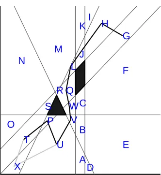
The Figure 2.2.4 shows an example with a single obstacle in a four-way-connected graph. Two paths,τ1

andτ2, have the same initial vertex,vs. In the original graph, the goal vertex,vg of the two paths are the

same because they have the same coordinates. However, in theh-signature augmented graph, the goal vertex ofτ1would bev1g = (xg, yg,“r1+”). While, the goal vertex ofτ2would bevg2= (xg, yg,“ ”). So we have v1

g 6=vg2. In the same manner, the goal vertices ofH-signature (using the bump form in (2.2.3)) graph will

bev1

v

_s

v

_g

τ

₁

τ

₂

O

₁

ζ

₁

Figure 2.5: Example of augmented graph. The goal vertices of two different paths,τ1andτ2, have the same

Chapter 3

Trajectory Generation under

Topological Constraints

In this chapter, we present a method to generate an optimal trajectory restricted to a particular topology class. The optimality of the generated trajectory is achieved by formulating the trajectory generation problem as a Mixed-Integer Quadratic Program (MIQP) [84, 80]. As theH-signature is the homology class invariant function, we can find shortest paths with graph-search based planner [10]. But we cannot addH-signature constraints to optimal control because the gradient ofH-signature is zero almost everywhere. So, we intro-duce binary variables that not only encode information about the satisfaction of geometric constraints, but also incorporate information about the topology class. We will cleverly consider topology class constraints so that the suggested trajectory generation problem under topology class constraints can still be formulated as a MIQP. We illustrate the method with examples of minimum acceleration trajectory generation under differ-ent topology class constraints with potdiffer-ential application to differdiffer-entially-flat systems with a two-dimensional flat output space. The work in this chapter was performed in close collaboration with Dr. Koushil Sreenath and Dr. Subhrajit Bhattacharya. Much of the work in Section 3.2 and Section 3.3 were reported in [58] and [59], respectively.

3.1

Optimal Trajectory Generation

We consider trajectory planning in a compact subsetQ⊂R2of a plane. LetO ={o1, o2,· · · , ono}be a

set of convex, pair-wise disjointobstaclesinQ(The requirement of convexity of obstacles can be relaxed by considering a set of arbitrarily-shaped obstacles such that their convex hulls are pair-wise disjoint). Each obstacle oi ∈ O can be represented by a ni-sided convex polygon, whose faces define hyperplanes that

partitionQinto two half-spaces. A binary variable is used to indicate whether a point is on the feasible side of the hyperplane, as described in [80]. So a pointq∈ Qwill be feasible and will avoid collision with an obstacleoiif there is at least one facef ∈[1, ..., ni]satisfyingni,f·q≤si,f. Whereni,fis a normal vector

to thefth_{face of obstacleo}

ipointing inward, andsi,f=ni,f·p, for an arbitrarily chosen pointpon thefth

p

q

Inside

Outside

n

i,f

o

i

f

th

face

→

(a)

p

q

Inside

Outside

n

i,f

o

i

f

th

face

→

(b)

Figure 3.1: The normal vector,ni,f, of thefthface of obstacleoiis pointing inward.pis an arbitrary point

on thefthface. (a) An example ofq∈Qwhenbi,f = 0. (b) An example ofq∈Qwhenbi,f= 1.

b=[0,1,1]

b=[1,0,1]

b=[0,0,1]

q

k−1

q

k

q

k+1

(a)

b=[0,1,1] b=[0,0,1]

b=[1,0,1]

b=[1,0,0]

(b)

a given point is feasible with respect to obstacleoiif

ni,f·q≤si,f−δr+M bi,f for f = 1, ..., ni (3.1.1) ni

X

f=1

bi,f≤ni−1,

wherebi,f ∈ {0,1}are binary variables (withbi,f = 0indicating that the point lies on the feasible side of

thefthface of theithobstacle as shown in Figure 3.1(a)), andM > 0is a large positive number. δr≥0

is the radius of the disk encircling the finite-sized robot, along with some safety-padding around it. The second inequality in (3.1.1) implies that the pointqwill be feasible with respect to at least one face,i.e.,

for a given i, there exists at least onef such thatbi,f = 0. Although (3.1.1) is a sufficient condition for

feasibility, this formulation breaks upQinto overlapping subsets as shown in Figure 3.2(a). The first three plots in Figure 3.2(a) illustrate that the subset corresponding tob = [0,0,1]is the intersection of the two subsets corresponding tob= [0,1,1]andb= [1,0,1]. Considering the segment of trajectory in the last plot of Figure 3.2(a), the binary variable vectorbk, corresponding to the pointqk, is not unique, but could be any

ofb = [0,1,1],b = [0,0,1]andb = [1,0,1]. As a result, we can have the same trajectory (represented by the points on it) described by different sets of binary variables. Such duplication increases the size of the feasible region in the space of binary variables, resulting in redundant searches, and larger computation times. To eliminate such cases, we introduce some additional inequality constraints to build disjointed cells like in Figure 3.2(b),

−ni,f·q≤ −si,f+δr+M(1−bi,f)forf = 1, ..., ni. (3.1.2)

The first inequality of (3.1.1) only guarantees that the pointqis on the feasible side or outside offth_face

whenbi,f= 0. But the constraint (3.1.2) enforces that the pointqbe on the other side whenbi,f = 1. Thus,

the feasible region,Q, is partitioned into disjoint cells, each of which is bounded by hyperplanes defined by the faces of the obstacles. (see Figure 3.2(b)). Moreover, each cell can be identified by a unique vector of binary variables,b= [bT1, . . . , bTno]

T _whereb

i= [bi,1, . . . , bi,ni]

T _{∈ {0,1}}ni_.

We parametrize the trajectory by splicingNssegments of trajectories, each parametrized by linear

com-bination ofNp+ 1basis functions, q(t) =

Np

X

k=0

cj,kek(t−tj) for tj≤t < tj+1, (3.1.3)

forj ∈ [0, ..., Ns−1],0 = t0 ≤ t1 ≤ ... ≤ tNs = tf. Whereek(t)is any basis function andcj,k are

coefficients. So the whole trajectory is union of Ns subtrajectories The trajectory is restricted to bekr

-times differentiable at the junction of each of the segments of trajectories,q(tj), forj ∈ [1, ..., Ns−1].

Further, obstacle avoidance is achieved by enforcing (3.1.1) at some equally distributed intermediate points on each segment of trajectories. we choose the cost function to be the integration of the square of the norm ofrth-derivative of the trajectory:

J(c) = Z tf

t0

drq(t) dtr

2

wherec = [cT₀, ...cT_N

s−1]

T_{, andH depends only on the choice of the basis functions (note that we could}

choose a cost function that is a weighted sum of different order derivatives, and still keep it quadratic in

c). The optimal trajectory generation problem can then be simplified as the following MIQP (Mixed-Integer Quadratic Program),

min c,eb

cTHc (3.1.5) s.t. Afc+Dfeb≤gf

Abeb≤gb

Aeqc= 0

whereebis the vector formed by stacking all the binary vectors,bk, corresponding to the intermediate points, qk, of the trajectory and hence is a coarse representation of the continuous trajectoryq(t). The first inequality

captures the feasibility constraints of (3.1.1) for the intermediate points, the second inequality captures the constraint on sum of binary variables in (3.1.1), andAeqc = 0imposes rthorder differentiability at the

junction of the segments of trajectories and the boundary conditions of initial configuration,q(0) =q0and

final configurationq(tf) =qf.

Now in the following sections, we will discuss how to add homology or homotopy class constraints on this trajectory generation problem while maintaining the MIQP formulation.

3.2

Optimal Trajectory with Homology Class Constraints

To find an optimal trajectory in a specific homology class, we can then add some topological constraints. If we add a constraint on theH-signature, which we described in the Chapter 2, such that theH-signature of the trajectory,H(q), should be some desiredHd. However, all the form ofH-signature (2.2.1), (2.2.3) and

(2.2.5) are the nonlinear equations of the trajectory. So, the quadratic program (3.1.5) becomes a non-convex problem with this homology class constraints. Furthermore, the gradient of the new constraint,H = Hd,

will be zero almost everywhere, because the value of theH-signature does not change within a particular homology class, (i.e. the range of theH-signature is a set of discrete variables). So, the resulting problem is a non-convex problem, which is numerically hard to solve based on gradients of cost and constraints. So, we need a different way to enforce topological constraints.

3.2.1

Algorithm Description

In this Section, we will describe our algorithm to generate the optimal trajectory with homology constraints while ensuring that the problem remains a MIQP.

Additional feasibility condition

We start by noting that the feasibility (with respect to obstacles) of each intermediate point on the trajectory does not guarantee the feasibility of the whole trajectory. Consider an example with only one parallelogram obstacle as shown in Figure 3.2.1. In Figure 3.2.1, two adjacent intermediate points,q1 andq2, are both

f=1

f=2

f=3

f=4

o

1

q

1

q

2

q

3

q

4

q

5

Figure 3.3: An example of parallelogram obstacle.f is the index of each face. Red and magenta curves are infeasible trajectories between two feasible configurations,q1andq2. Adjacent intermediate points(q3,q4

andq5) are satisfying additional constraint.

connecting two points. Of course, the optimal trajectory could be feasible like the green curve. However, the line segment connecting the two points (the magenta curve) is infeasible. To avoid such undesirable cases, we need additional constraint between adjacent intermediate points. The curves in Figure 3.2.1 illustrates this additional constraint: Considering the corresponding binary variables of each point,q3is only feasible

with respect to facef = 1and the next intermediate point,q4is also feasible with respect to the same face.

So, the line segment, connecting these two points is also feasible with respect to facef = 1. Moreover, both

q5and its previous point,q4, are feasible with respect to facef = 2. So the line segment joining them is also

feasible. In contrast, consider the case ofq1andq2in Figure 3.2.1. These two adjacent intermediate points

do not share feasibility with respect to a common face –q1is feasible with respect to only facef = 4and q2is feasible with respect to only facef = 1. So we cannot guarantee the feasibility of the line segment

connecting these two points.

The above discussion suggests an additional constraint that two consecutive intermediate points should share a common hyperplane with respect to which they are feasible, and this should hold true for each obstacle. In other words, the binary variables corresponding to the adjacent intermediate points should either be the same or differ by only one component, and this condition should be satisfied with respect to all obstacles. This constraint then guarantees the feasibility of a straight line segment connecting the two intermediate points. We writeb(o,k)to describe the vector of binary variables for thekthintermediate point

formed by stacking together the binary variables for the different faces of theothobstacle (thus, it is ani

-sized sub-vector ofeb). Thus the constraint involving thekthandk+ 1thintermediate points with respect to othobstacle can be describe as

b(o,k)−b(o,k+1) 2 2=

X

b(o,k)·b(o,k)+b(o,k+1)·b(o,k+1)−2b(o,k)·b(o,k+1) (3.2.1)

=Xb(o,k)+ X

b(o,k+1)−2b(o,k)·b(o,k+1)

where,P

bdenotes the sum of the elements of a binary vector, and the last equality holds sinceb·b=P b

for a vector of binary variables,b ∈ {0,1}n_{. This additional constraint on the gradual change of the binary}

variables along the trajectory plays an important role in formulation of a new h-signature based on binary variables, as described in the next section. However, this constraint is quadratic in the binary variables, and we will discuss how we can reduce this constraint to a linear one in Section 3.2.1.

DefineH-signature

To find an optimal trajectory contained in a specific homology class, theH-signature defined in Chapter 2 can be used. However, these function are homology class invariant whose gradients are zero almost everywhere. So, the homology class constraints based onH-signature are not proper for gradient-based numerical solvers. However, we chooseH-signature of (2.2.5) for this work. We can choose arbitrary reference ray of each obstacle but for convenience of calculation and notation, we choose the reference ray as the extension of face

f = 1in the direction of the last facef =nfas shown in Figure 3.2.1. Also, for the consistency of sign of

winding number, the faces are numbered in counterclockwise direction like Figure 3.2.1. So, for a givenit

obstacle, theH-signature will be

Hi(q(t)) = Z tf

t0

υ(di·(γ(t)−ζi))δ(ni,1·(γ(t)−ζi))dt (3.2.2)

whereni,1is the normal vector the of the1stface of theithobstacle anddi=R π₂

ni,1is the direction of

reference ray, which is rotating the normal vector by π₂ andζiis an arbitrary point on the1stface. However,

the gradient of this integration will be zero almost everywhere and is not proper constraint. Here, we need to focus on the fact that geometric meaning of this integration is counting the number of times the trajectory crosses the given reference ray. Moreover, this reference ray is one the the boundary or hyper plane that splits the feasible space into cells. So the change of binary variable corresponding to the first facebi,1will

give us alternative way to integrate (3.2.2).

From this fact, it is obvious that we need to accumulate the value ofbi,1,k+1−bi,1,kfor∀k(where bybi,j,k

we mean the binary variable for thekth_{intermediate point corresponding to thej}th_{face of thei}th_obstacle).

However, to avoid counting the number of intersection with the the other ray obtained by extending the face

f = 1in the other direction (the green line in Figure 3.2.1), we need to count the case when the two adjacent intermediate points are infeasible with respect to the second facef = 2,i.e. bi,2,k+1=bi,2,k = 1. So, the H-signature with respect to an obstacle,oi, will be

Hi(eb) = X

k

bi,2,k+1+bi,2,k

2 (bi,1,k+1−bi,1,k). (3.2.3)

=X

k

bi,2,k(bi,1,k+1−bi,1,k)

The second equality of above equation holds becausebi,2,k+1=bi,2,kwhenbi,1,k+1 6=bi,1,kdue to the

constraint we defined in (3.2.1). TheH-signature with respect to all obstacles will beH = [h1, ..., hno]

T_,

wherenois the number of obstacles. However, this newH-signature is also quadratic in binary variables.

f = 1

f = 2

f = 3

o

(+1)

(−1)

(+0)

(−0)

Figure 3.4: An example of calculating the h-signature with respect to a triangular obstacle.

Substitution binary variables

As the new constraint in (3.2.1) and the H-signature in (3.2.3) are quadratic with respect to the binary variables, we introduce somesubstitution binary variablesthat represent the product of two binary variables. For example, consider the product of two binary variables,bi·bj, forbi, bj ∈ {0,1}. Then, we substitute bi·bjwith a new binary variabledij ∈ {0,1}, on which we impose the following three inequalities,

dij≤bi , dij ≤bj , −2 +δ+bi+bj≤dij (3.2.4)

where0< δ <1is a design parameter. The first two inequalities in (3.2.4) enforcedij = 0whenbi= 0or bj = 0, respectively. And the last inequality enforcesdij = 1whenbi=bj = 1, because0< δ≤dij. So

the above three constraints let us perform the substitutiondij =bi·bj. Letdbe the vector of substitution

variables with which we need to replace all the quadratic terms in (3.2.1) and (3.2.3). Then we can rewrite the feasibility conditions of substitution binary variables, (3.2.4), as

Af,deb+Bf,dd≤bf. (3.2.5)

Then we can rewrite the quadratic constraint of (3.2.1) for the whole trajectory as

Ao,keb+Bo,kd≤bo,k (3.2.6)

for alloandk. And the h-signature calculation of (3.2.3) becomes the following linear equation

Hi =Ai,hd. (3.2.7)

Finding Optimal Trajectory in a given Homology Class

Since our goal is to design optimal trajectory with homology constraint, we can impose the new constraints of (3.2.5), (3.2.6), and (3.2.7) to the optimal trajectory generation problem (3.1.5) to formulate a new MIQP as follows

min c,eb, d

cTHc (3.2.8) s.t. Afc+Dfeb≤gf

Abeb≤gb

Adeb+Bdd≤bf

Aoeb+Bod≤bo

Aeqc= 0

Ahd=Hd

whereeb andd are vectors of binary variables as described earlier. The third inequality is the condition

of substitution variables (3.2.5), the forth inequality is for additional feasibility constraint for continuous change of binary variables (3.2.6), and the last equality is for the homology constraint with respect to all obstacles (3.2.7). As the resulting problem is MIQP, we can get an anytime solution to this problem through numerical solvers like CPLEX [52]. However, we need enough number of segments of trajectories (Ns) and

basis function (Np) to be able to obtain a feasible trajectory in the given homology class.

Proposition 3.2.1 (Completeness Guarantee). Suppose there exists an arbitrary trajectory τ (dark blue curve in Figure 3.5(a)), not touching any of the obstacles, in the homology class represented by theH

-signature of Hd, that crosses the cell boundaries (i.e. the hyperplanes)m or less number of times (for avoiding ambiguity we assumeτ is generic and that it does not pass through the intersection of2or more

hyperplanes). With the choice of basis functionsek(t) =tkin(3.1.3), and withNp> r, it is then sufficient to chooseNs= 2r(m−1) + 1in order to guarantee existence of a solution for the problem in(3.2.8)(i.e. all the conditions being satisfied, and with finite cost).

Sketch of Proof.

Consider them−1consecutive cells thatτpasses through. We choosem−1points,q0

1, q02,· · ·, qm0−1,

respectively in the interior of each of these cells. Now, two such consecutive cells together form a convex region (bounded by the hyperplanes the cells are individually bounded by, except for the one hyperplane that separates them). Thus, the piece-wise linear curve formed by joining these consecutive points (call this q0_{) give a trajectory consisting of m segments (cyan curve in Figure 3.5(a)), connecting the initial}

and final points, not intersecting any of the obstacles, and is continuous (i.e. 0th order differentiable). The affine segments are permitted by the choice of the basis functions (the parametrization may be chosen arbitrarily), thus giving values of coefficients,cj,k, in (3.1.3) that describe this trajectory. Those, along with

the binary vectors corresponding to each of these points, satisfy all the conditions in (3.2.8), except for the differentiability conditionAeqc= 0.

Figure 3.5: Starting from a piece-wise linear curve (cyan), we can progressively add points, to make the trajectory smoother by increasing the order of differentiability by one at each step.

possible to achieve with just an unit increase in the degree of the basis functions (which is evident by looking at the individual componentsq0

x(t)andq0y(t), as illustrated in Figure 3.5(c)) – in this case, going from linear

to quadratic (it is always possible to find a parabola that has two given lines with bounded slope as tangents, and then scale it down such that the contact points with the tangents lie within a small ball around the point of intersection of the lines).

Thus, now we have a new trajectory (call thisq1_{), that is smooth everywhere, but not twice differentiable}

(red trajectory in Figure 3.5(b)). However, we can continue the same process of smoothening the derivatives ofq(t)by adding points in a small neighborhood of the originaltj’s, doubling the number of intermediate

points at every step. The choice of this neighborhood can be arbitrarily small to ensure that the added points remain in the interior of the same cell. Continuing this until we have rthorder differentiability requires

2r_{(m−1)intermediate points. In this way, we can construct a trajectory that satisfies all the conditions of}

(3.2.8).

Computational Complexity

The resulting optimal trajectory generation problem is a MIQP, which can be solved by an anytime solver like CPLEX. Thus, if there exists a feasible solution, it will be found by CPLEX. Moreover, with additional time available for computation, a lower cost solution can be found. However, the computation time will increase with the complexity of the given MIQP. So, in this section, we will discuss the computational complexity of the trajectory generation problem (3.2.8). The number of continuous variable in the problem is

nc = 2(Np+ 1)Ns (3.2.9)

where there areNssegments of trajectories ofNp+1basis function for eachxandy. However, some equality

constraints to satisfy initial and final configuration and the continuity between segments of trajectories will reduce the actual number of continuous variables by searching the null space ofAeqof (3.2.8). Again, the

number of binary variables to describe feasibility with respect to each face of obstacle is