of a Class of Artificial Neural Network
a PhD. thesis by
Paul Houselander 12th May 1991
Dept Electronic and Electrical Engineering University College London
All rights reserved
INFORMATION TO ALL USERS
The qu ality of this repro d u ctio n is d e p e n d e n t upon the q u ality of the copy subm itted.
In the unlikely e v e n t that the a u th o r did not send a c o m p le te m anuscript and there are missing pages, these will be note d . Also, if m aterial had to be rem oved,
a n o te will in d ica te the deletion.
uest
ProQuest 10610958
Published by ProQuest LLC(2017). C op yrig ht of the Dissertation is held by the Author.
All rights reserved.
This work is protected against unauthorized copying under Title 17, United States C o d e M icroform Edition © ProQuest LLC.
ProQuest LLC.
789 East Eisenhower Parkway P.O. Box 1346
Artificial neural networks (ANNs) are highly interconnected systems of simple processing cells the inspiration for which stems from the biological brain. In this thesis we will consider the motivation design and implementation of a particular class of these structures based on the Radial basis function (RBF) and in particular, the Gaussian function. Chapter 1 introduces some basic concepts, the motivation behind ANN research and a summary of the various landmarks which have led to the intense international interest that the subject now enjoys. Chapter 1 also introduces the RBF neuron which will be used in the chapters to follow and considers the related field of conventional pattern recognition.
Although the link between the artificial and biological systems is somewhat tenuous, we shall endeavour to form a connection between the different ANN designs covered in this thesis and a simplified subjective model of perception. Hopefully, this will enable the reader to obtain a better perspective on the role that each network would play in an artificial perceptual system.
Please note th at in the following, " lines" refer to the number of text lines (including headings and equations) only.
The following should be inserted at the position specified.
Page 26 line 2 immediately after . . . longer agree on its classification.
In essence, the reason for poor generalisation is the overfitting or underfitting of data. For example, if we consider that data is derived from a polynomial, if we attempt to model this polynomial using a polynomial of incorrect order, an exact fit is unlikely to be achieved. In the case of underfitting the data, this is due to insufficient terms. In the case of overfitting the data, one might expect that terms, which are beyond the terms in the polynomial to be modelled, would be set to zero by the adaptive process. This requires more data points than would otherwise be the case and this point is demonstrated by the following simple example: If the function to be modelled is linear, only two unique data points are required to specify the equation exactly. If we model this linear equation by a quadratic, the two data points would specify a family of curves with one member of that family being the required solution with each solution being equally valid using only the information obtained from the two data points.
Page 31 line 23 after word 9 "to".
Page 58 Line 8 immediately after . . . the distribution of the input.
In particular, the combination of RBFs are attempting to model or "fit" the probability distribution of the training data.
The following should replace the text at the position specified.
Page 8 line 3 word 4 "are". Page 18 line 5 word 2 "differential". Page 22 line 1 word 3 "scalar". Page 26 line 12 word 12 "106". Page 28 line 10 word 4 "Manhattan". Page 30 line 13 word 14 "one". Page 36 line 38 word 12 "and". Page 43 line 2 word 14 "enclose". Page 46 line 16 word 10 "is". Page 47 line 1 word 4 "frequencies". Page 101 line 8 word 8 "which".
Page 138 line 23 The sentence beginning. . . This effectively removes the difficulty. . .
This is sufficient for inputs that are not disjoint from the initial area in the input state space from which training data was first Page 56
afa+1) = Z,- [fy+l)*1.! [% )*] - W fa+m
= nj a /n y).(n,+l)-> + 2, [(n,+l)->.(*,</>,+1)2 + nyW^njp-) - ]
replacing W Jnj) using equation 2.5.8
= 1)'1 + Z,- [(ny+D -U X ^+l)2 +nj .(nfH(nJ+l).Wij{nJ+1) - X ^-fl))*)) - W f a + m
- nj.afnj).{nj¥I)’1 + £,• [(nj+1)-l.(Xi{nfrl)2 +
n/».((/l;+l)2.W.<n74-l)2 - 2 . { n ^ \ ) X ^ \ y W i}{ n ^ \) + X ^ + I P ) - ( n ^ l j .W ^ + l ) 2)]
= nj.aJ(nJ).(nJ+ l ) 1 + X,- [n;-1.(/i/ 4-l)-1.((n/ +-l)Jf/.(n.-t-l>2 - ^ .(n ^ j.W y ty + l)2 - 2 . { n f r \ ) X ^ \ ) . W i}{ n ^ \) + ( n ^ l p . W ^ + l ) 2) ]
(2.5.10)
(2.5.11)
(2.5.12b) (2.5.12a)
(2.5.12c)
n;,a /n ;).(/i,+l)-i + Z. [n / i.(«;+l)-i.((n;+ l ) J f ^ - H ) 2 + (n ^lj.W ^n+ l)2 - 2.(n;+ l)X 1(n;+ l) .^ < « ;+l))] (2.5.12d)
^ n y.a/n;).(n,+l)-i + Zt- [ n - K X ^l)2 + W ^ + l ) 2
-simplifying by using the identity of eqn. 2.5.1 and replacing ny by p.n; as before:
(2.5.12e)
=> afnj¥ 1) = ($.nj.aJ(nJ).($.nj + I ) 1 + nef/ny+1 )).£ :« /1 (2.5.13)
obtained. For training data that is disjoint, the associative memory will require parallel inputs from other sensory sources as well as feedback from higher brain functions such as hypothesis evaluation, to enable the correct association to take place.
The following text should be deleted from the position specified.
Page number
A c k n o w le d g e m e n ts ... 8
N o ta tio n , sy m b o ls a n d a b b re v ia tio n s u s e d ... 9
1 Notation and symbols... 9
2 Operators... 11
C h a p te r 1 A rtific ia l n e u r a l n e tw o rk s , m o tiv a tio n a n d c o n c e p ts... 14
1.1 The need for an alternative to the sequential computer... 15
1.2 The biological neural network... 17
1.2.1 The dynamics of neuron operation... 18
1.2.2 Modelling the biological neuron... 20
1.3 The history of A N N s... 20
1.4 Semantic networks: the application of distributed systems to cognition... 23
1.5 Basic concepts in pattern recognition... 23
1.5.1 Learning by exam ple... 24
1.5.2 When does an "A" become an "H "... 24
1.5.3 Generalisation and the problem of inference... 25
1.5.4 The input state space... 26
1.5.5 Decision boundaries and decision surfaces... 27
1.5.6 Distance m etrics... 27
1.6 Conventional classification techniques... 28
1.6.1 The linear classifier... 29
1.6.2 The <|> machine... 29
1.6.3 The piece-wise linear classifier... 30
1.6.4 The nearest neighbour classifier... 30
1.6.5 The k nearest neighbour classifier... 30
1.6.6 The c-means and fuzzy c-means clustering algorithms .. 31
1.6.7 The compound and Gaussian classifiers... 31
1.7 Outline of thesis, a simple model of perception... 33
1.8 An alternative to the first order model, the radial basis function 35 1.9 Summary... 38
C h a p te r 2 T h e firs t level o f p e rc e p tio n : S e lf-o rg a n is a tio n a n d f e a tu r e e x t r a c t i o n ... 40
2.1 Pre-processing... 41
2.2.2 The application of Kohonens feature map to phoneme
extraction... 45
2.3 Linskers model: Feature discovery by competitive learning... 47
2.3.1 Training the Linsker model... 48
2.4 Adaptive resonance theory model 1 (ART 1)... 49
2.4.1 The operation of ART 1... 50
2.5 Feature Extraction using the Radial basis function (RBF) neuron 51 2.5.1 A simple statistical training algorithm ... 54
2.5.2 Initialising the adjustable parameters... 56
2.5.3 Simulation results... 57
2.7 Summary... 59
C h a p te r 3 T h e seco n d level o f p e rc e p tio n : M a p p in g N e t w o r k s ... 61
3.1 The single layer perceptron... 61
3.1.1 Perceptron convergence procedure (perceptron training algorithm)... 63
3.2 Optimisation and gradient descent... 64
3.2.1 Tabulation methods... 64
3.2.2 Sequential methods... 65
3.2.3 Linear methods... 65
3.2.4 Univariate se arc h ... 65
3.2.5 Hooke and Jeeves method... 65
3.2.6 Gradient m ethods... 66
3.3 The multilayer perceptron... 67
3.3.1 The backpropagation training algorithm... 69
3.4 A two layer network based on the radial basis function... 74
3.4.1 Training the RBF two layer netw ork... 74
3.4.3 Comparing the MLP with the RBFE and RBFS networks... 77
3.5 Counterpropagation... 80
3.6 Statistical training schem es... 81
3.6.1 Simulated annealing... 81
3.6.2 The Boltzmann machine... 82
3.6 Sum m ary... 84
C h a p te r 4 T h e th ir d level o f p e rc e p tio n : A sso ciativ e m e m o ry ... 86
4.1 Binary associative memories... 87
4.2 The Hopfield Network... 88
4.2.3 Calculating the upper and lower bounds on capacity . . . . 96
4.2.4 Calculating the upper and lower bounds on associativity... 100
4.2.5 Using the Delta rule to train the Hopfield n etw o rk ...106
4.2.6 The associativity of the delta trained netw ork...107
4.2.7 High order correlations (HOCs)...108
4.2.8 Using high order non-linearities in the three layer Hopfield netw ork... 109
4.2.9 Using other non-linearities in the three layer Hopfield network... 110
4.3 The Hamming Network... 113
4.3.1 Programming the Hamming network...113
4.3.2 Determining suitable values for a and P...115
4.3.3 Calculating the maximum number of iterations to reach a solution... 116
4.3.4 Improving the structure of the Hamming network...117
4.3.5 Reducing the connections between layer 1 and layer 2 ... 118
4.3.6 Reducing the number of connections in the selection layer... 120
4.3.7 The performance of the improved Hamming network... 120
4.4 An RBF associative memory... 121
4.5 Summary... 123
Chapter 5 The fourth level of perception: Hypothesis
E v a l u a t i o n ... 1265.1 Interactive activation and competition (LAC)... 127
5.2 The bidirectional associative memory (BIAM )... 129
5.2.1 Training the bidirectional associative memory... 130
5.2.2 The performance and stability of the BIAM ...131
5.3 A hypothesis evaluator based on the Hamming network... 132
5.4 Summary... 133
Chapter 6 Realising a simple model of perception using RBF
n e tw o rk s a n d th e u n ific a tio n o f th e ir d e sig n ... 1346.1 Feature extraction... 134
6.2 Classifiers and mapping networks... 135
6.3 Associative memories and hypothesis evaluation... 138
6.4 Unifying the RBF networks designed to implement the four levels of perception...139
7.2 Parallel hybrid analogue/digital designs...149
7.2.1 A BICMOS circu it... 149
7.2.2 A time-multiplexed circuit... 150
7.2.3 Pulse stream arithmetic... 153
7.3 Sequential digital implementations...154
7.3.1 The development of a neural network language (NNL) translator... 155
7.4 Parallel and special purpose implementations...157
7.4.1 General-purpose architectures... 157
7.4.2 Programmable systolic c h ip ... 159
7.4.3 Connection machine...159
7.4.4 HNC A N Z A ... 160
7.4.5 TRW Mark HI & I V ... 160
7.4.6 IBM NEP... 160
7.4.7 WISARD... 161
7.4.8 NETSIM... 162
7.5 A pseudo-asynchronous re-configurable architecture (PA RA) 163 7.5.3 The design of a P A R A ... 165
7.5.4 Implementing the two layer RBF using a PA R A 168 7.6 Summary...172
C h a p te r 8 S u m m a ry , c o n clu sio n s a n d f u tu r e w o r k ... 173
8.1 A review of the previous chapters contained in this thesis...173
8.2 Future directions... 178
R e f e r e n c e s ... 180
A p p e n d ix A N e u ra l n e tw o rk la n g u a g e u s e r g u i d e ...186
A1 The structure of a NNL program ... 189
A2 Functions...192
A3 Keywords...193
Reading for a PhD is not the retirement occupation envisaged by industrial onlookers. Having personally experienced both a working environment and a PhD environment, the two a very different. In industry, the normal practice is to go to work in the morning, work throughout the day and then go home and socialise with friends in the evening. When reading for a PhD, one goes to college in the morning (so far so good and yes, PhD students are aware that the sun rises in the east !) socialise with friends and then go home, feel guilty about the days lack of progress and slave over a hot computer into the small hours. At work, one seldom feels the intense excitement experienced from a new discovery. Conversely, one seldom experiences the extreme depression when an experiment comes up with the wrong answer (in the sense that it disagrees with your theoretical calculations, which are of course, sacrosanct) or you stumble across a twenty year old paper in a dusty library mezzanine which outlines exactly your "new" discovery. It is these highs and lows that are the essence of research and which stand it apart from conventional employment.
Having finished the PhD (or did the PhD finish me ?), I can reflect on a very enjoyable three years. I would like to thank Dr John T. Taylor for the dedication of his supervision and his uncanny ability to instantly spot a split infinitive or tautology in my very broken English. I would like to express my gratitude for the friendship and support of my fellow PhD candidates Vishank Patel and Patrick John Wright. I would also like to thank the secretarial staff for their assistance and their ability to light up the dullest day. I would also like to acknowledge the many interesting discussions with David Selviah (University College London) on the subject of associative memories and thank Graham Tattersall (University of East Anglia) for introducing me to this extremely interesting and diverse subject.
In every science and engineering discipline there is inevitably mathematics to be considered. However, over the many years that the subject of artificial neural networks (ANNs) has been studied, a plethora of symbols and notation has emerged. In particular, the ANNs to be described in this thesis are normally defined using a variety symbols which make comprehension of the mathematics involved unnecessarily complicated. To simplify this, we shall endeavour to use a concise and consistent notation. The notation is based on the assignment to a particular layer of a unique index. For example, parameters referring to the input layer (layer 0) will be denoted by the subscript t, parameters pertaining to layer 1 will be denoted by the subscript j and so on. With this scheme, there is a problem with feedback connections from a neuron to itself. Where this occurs, an extra layer of linear neurons will be added. This keeps the notation consistent whilst keeping network operation unchanged. The notation and symbols used are defined thus:
1 Notation and symbols
Subscripts
c Subscript denoting variables that pertain to the constant input or node whose output is set to unity.
ijjc j Subscripts denoting variables that pertain to layer 0 (input layer), layer 1, layer 2 and layer 3 respectively whose range is 1 to N.
m Subscript denoting a particular memory.
s Subscript denoting a particular iteration (or snapshot in time).
Variables
A The weight which is a reciprocal measure of the radius of a RBF neuron.
a The weight which determines the radius (variance) of a RBF neuron.
C The node exhibiting the greatest excitation in a Kohonen network.
c The consensus in a Boltzmann machine, or the correlation noise in an associative memory.
Cov The covariance.
E The LMS error.
AT The corrected number of memories when calculating bounds on capacity and associativity.
N The number of nodes in a particular layer.
NSC The neighbourhood surrounding node C in a Kohonen network.
n A variable that is incremented with each iteration (also a measure of time, as the time for one iteration is arbitrary and can therefore be set to unity).
nmax Maximum iteration time in a Hamming network.
net The total input to a particular neuron.
O The output of a neuron.
R The required output.
r Represents the number of memories that are aligned with the exemplar in an associative memory calculation.
S A stored memory, the first subscript refers to the memory and the second subscript refers to the bit within that memory.
s The required signal in an associative memory (i.e. the correlation of the probe with the exemplar).
T The temperature or degree of randomness
U,V N dimensional vectors.
W The connection weight between two layers.
X An external input to the network.
AA The incremental update for weight A.
A a The incremental update for weight a.
Av Change in output for a 1 bit change in input.
AW The incremental update for weight W.
a , (3 ... X Constants.
a The standard deviation of a distribution.
o 2 The variance of a distribution.
Functions
BIPT The bipolar threshold transfer function of a neuron defined thus:
BIPT(jt) = + l ; j t £ 0
BIPT(jt) = -1; jc < 0
expO The exponential function.
fQ The transfer function (usually non-linear) of a neuron.
InO The natural logarithm.
maxO Returns the subscript of the vector element which has the maximum positive value.
min() Returns the subscript of the vector element which has the minimum positive value.
QLIN The quasi-linear transfer function of a neuron defined thus:
QLIN(jc) = jc; jc > 0
QLIN(jc) = 0; jc < 0
UNIT The unipolar threshold transfer function of a neuron defined thus:
UNIT(jc) = 1; jc > 0
UNIT(jc) = 0; jc < 0
Operators
—> Is replaced by.
I I Absolute value or determinant of a matrix.
< > Ensemble average.
p(a) Probability of alignment in an associative memory calculation.
I,- [] The summation over all values of the subscript (in this example i).
2 Abbreviations
4QAM Four quadrant analogue multiplier.
Adaline Adaptive linear network.
AI Artificial intelligence.
ANN Artificial neural network.
ASIC Application specific integrated circuit.
BIAM Bidirectional associative memory.
BICMOS Bipolar complementary metal oxide semiconductor.
CC Compound classifier.
CMOS Complementary metal oxide semiconductor.
EEPROM Electronically erasable programmable read only memory.
FSC Final neuron output storage capacitors.
HIDR Hebbian initialised delta rule.
HN1 Hopfield network variant 1.
HN2 Hopfield network variant 2.
HOC High order correlations.
IC Integrated circuit.
IFF If and only if.
LMS Least mean square.
MER Mean error rate.
MIPs Million instructions per second.
MOS Metal oxide semiconductor,
ms Millisecond.
mV MilliVolt.
NEP Network emulation processor.
NNC Nearest neighbour classifier.
NNL Neural network language.
PARA Pseudo-asynchronous re-configurable architecture.
PCP Perceptron convergence procedure.
PE Processing element.
PSC Programmable systolic chip.
RBF Radial basis function.
RBFE Radial basis function mapping network based on hyperellipsoids.
RBFS Radial basis function mapping network based on hyperspheres.
RISC Reduced instruction set computer.
SORBFN Self-organising radial basis function network.
SWSC Synaptic weight storage capacitors.
TSC Temporary neuron output storage cells.
VLIW Very long instruction word.
VLSI Very large scale integration.
vNM von Neumann machine.
WRT With respect to.
ZMIDR Zero matrix initialised delta rule.
Artificial
neural
networks,
lilllisl
Artificial neural networks (ANNs) are inspired by the complex systems of nerve cells or neurons which form the animal brain and the massive number of interconnections which pervade its structure. They offer radical departure from the paradigm of conventional computing replacing sequential operations by highly parallel processes, explicit programming by implicit learning algorithms and knowledge intensive analysis with example oriented training. Essentially, an ANN is a non-biological realisation of a highly interconnected system of simple non linear processing nodes, each node exhibiting properties similar to those found within the biological brain. A formal definition of a neural network is provided by Hecht-Nielsen [Hec90]:
Definition 1.1
arbitrarily with the restriction that it must be completely local: that is, it must depend only on the current value o f the input signals arriving at the processing element via impinging connections and on values stored in the processing element's local memory.
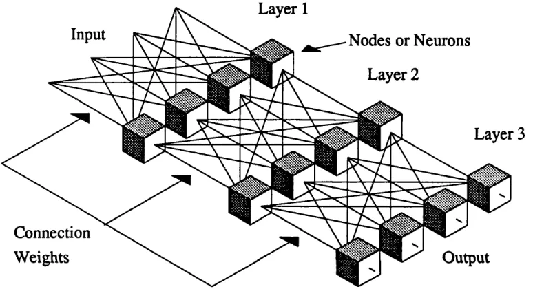
A representation of an ANN can be seen in Fig. 1.1. The network consists of a number of layers (in this case 3), with each layer containing a number of nodes or neurons. The efficacy of the connections which interconnect the layers dictate the
Layer 1
Input Nodes or Neurons
Layer 2
Layer 3
Connection
Weights Output
Fig. 1.1 Diagram showing the structure of a typical ANN.
response of a particular network and allow networks which are structurally identical to operate quite differently. As we shall see later, the method of training these connections determines, to a large degree, the performance and function of the various ANN models.
The subject of ANNs has had a long chequered history with several peaks and troughs in research interest. To understand the recent resurgence of interest, we must first explore the failings of conventional computing techniques.
1.1 The need for an alternative to the sequential computer
circuit (IC) manufacture which has led to a reduction in the minimum feature size of components. A natural consequence of their proliferation is a low manufacturing cost and this means that a powerful desk top system is relatively inexpensive when its specification is considered. With this back drop there would seem little requirement for an alternative technology. However, there are a large number of problems that sequential machines are inherently unsuited to solve. These problems, which come under the general heading of pattern recognition, may be characterised by the following properties [Hec88]:
(1) A mapping or transformation is required from regions with ill defined boundaries within a large input state space to a smaller but well defined output state space.
(2) In general there is no mathematical formulation to map the input domain onto the output domain.
(3) Many examples of the required mapping exist.
(4) The problems are normally generated by human beings.
An example of a task which has the above features is hand written character analysis [Hec88]. Interestingly, it is exactly these problems that the human brain seems most suited to solve and it is this fact which is the motivation behind the current research into the understanding of neural networks.
processor system as the upper bound on speed is limited by physical constraints (e.g. a signal travelling at the speed of light could not traverse further than 3mm in a single clock period of a 100,000 MIP machine). Therefore, a multiprocessor system must be employed. To program a multiprocessor system is non-trivial as it is extremely difficult (and often impossible) to partition an arbitrary task such that each processor achieves 100% utilisation. Many algorithms contain at least one sequential construct which means that the processing time may be limited to the speed of a single processor. The distinct advantage of ANNs is that they are inherently parallel structures and when implemented using appropriately designed multiprocessor systems will achieve 100% utilisation. It is therefore believed, that for pattern recognition at least, an artificial system based on structures similar to those found in the brain will offer a viable alternative to conventional techniques.
The link between the biological brain and the majority of artificial systems covered in this thesis is somewhat tenuous. This is due to the difficulty in modelling the highly complex electro-chemical processes found within the brain. To appreciate these difficulties, a discussion of neuron operation now follows.
1.2 The biological neural network
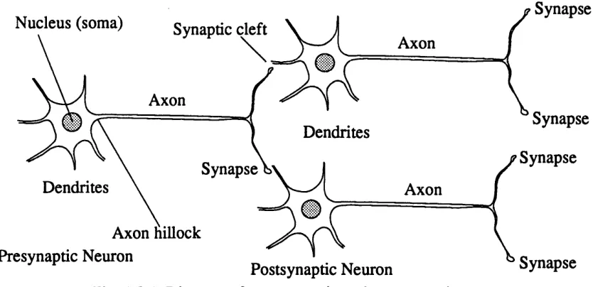
The human brain consists of a vast number of highly interconnected nerve cells or neurons. The total number of neurons is estimated to be 1011 and each neuron can have as many as 104 inputs from other neurons. The neurons themselves to a first order of approximation are simple in operation essentially summing both spatially and temporally the total input to the cell. This total input is then compared to a threshold and an output will be produced if the input exceeds the threshold. It is believed that the type of computation carried out is due to the connection pattern and the efficacy of each connection. The connection pattern remains virtually unchanged after the post natal period and it may be thought of as a “seed” to encourage the formation of specific computational functions within the brain lattice. This is brought about by the modification or training of the connection weights (synaptic weights) in response to the applied input stimuli. A diagram showing the neurons constituent parts can be seen in Fig. 1.2.1 and this figure should be referred to during the following discussion of neuron operation [Sam77,Nob86].
Nucleus (soma) Synaptic cleft
Dendrites
Synapse Dendrites
Axon hillock Presynaptic Neuron
Synapse
Axon
Synapse
Synapse
Axon
Postsynaptic Neuron
Fig. 1.2.1 Diagram of a presynaptic and postsynaptic neuron.
Synapse
1.2.1 The dynamics of neuron operation
change in the differential permeability of the membrane enabling the resting electrostatic potential to cause a large ionic current to flow. This effect is short lived however and the membrane potential soon returns to its resting state. Immediately following an action potential the region concerned is unable to be re excited for a period of approximately 1 ms and this is called the absolute refractory period. After that the reluctance to excitation diminishes with time (relative refractory period )and therefore the level of stimulation required to initiate an action also decreases until the pre-excitation threshold is reached. When an action potential occurs at the axon hillock the region on the axon adjacent to it has its threshold exceeded by the influence of the action potential and will in turn generate its own action potential. This process is repeated and the action potential travels at uniform speed along the axon. It should be noted that as the action potential only initiates the next action potential, no loss in amplitude will occur as the nerve impulse propagates along the axon. The reason for the refractory period now becomes clear. If the region which generates the action potential could be re excited immediately then the action potential would not only propagate away from the cell body but would also propagate towards the cell body. This process would be self sustaining and hence when a cell was initially activated it would burst into chaotic behaviour as action potentials oscillated back and forth along the axon and these could conceivably last indefinitely. The synapse which terminates the axon converts the nerve impulse, which is an electrical signal, into a chemical signal. Small packets called vesicles reside at the bulbous end of the synapse (bouton) and they contain the transmitter substance used to influence the membrane potential in the post synaptic neuron. When an action potential is received at the synapse, packets of neuro-transmitter are released and these drift across the synaptic cleft which separates the two cells. On the post synaptic side the differential permeability of the cell’s membrane is also altered and this causes a local change in the distribution of ions between the inner and outer membrane walls. This in turn affects the membrane potential whose effect is signalled and forms the graded response mentioned earlier. The type of chemicals found in the vesicles will dictate whether the post synaptic membrane will be either depolarised or hyperpolarised and hence whether an excitatory or inhibitory response is conveyed [Sam77, Nob86].
the position of a synapse on a dendrite affects the influence that it will have on cell activation. These and other anomalies make accurate simulation of biological neural networks practically impossible.
1.2.2 Modelling the biological neuron
From the previous section it would not seem feasible to accurately model the biological neural network although it must be stressed that work is being done to achieve this and significant progress has been made [Mea89,Tay89]. However, this does not preclude the use of neuron like characteristics being attributed to simple highly interconnected electronic circuits. It may be found that the subtleties of neuron operation mentioned in section 1.2.1 are unwanted consequences of the physical processes that nature is limited to using and that network operation is constrained to make allowance for them. The other extreme would be to say that the subtleties of operation allow a significant reduction in the processing elements required to perform a particular task. There is of course the possibility that the power of the brain is entirely due to the complexity alluded to and without this complexity the essence of brain operation is completely lost. It is hoped and believed that the actual situation is between these two limits. For example, it may be found that the early stages of sensory processing are relatively insensitive to the more esoteric aspects of neuron operation. However, the higher brain functions such as intuition and emotion may depend on them completely (eg quantum effects etc). Anyway, it is envisaged that by choosing carefully the characteristics of the artificial neuron, the early stages of network operation can be achieved with perhaps a small trade off in the required structural complexity.
1.3 The history of ANNs
As we have stated, neural networks as a subject has had a long and chequered history stretching back to the original work carried out on basic computational machines. It is interesting to note that John von Neumann whose name is synonymous with the architecture of sequential computers spent a large proportion of his time looking into highly parallel systems of brain like structures [von58]. In 1943 McCulloch and Pitts discovered what is in essence the simple characteristics of neuron operation and surmised from this that the brain is able to carry out any general computational task [McC43]. The simple first order model they used can be seen in Fig. 1.3.1 which is labelled using the notation to be used throughout this thesis and this model forms the basis of the majority of the ANNs so far devised.
Connecl
Output Oj
Fig. 1.3.1 Diagram of an Artificial neuron.
following two equations:
n etj= Zi [Xi-Wy + W.j] (1.3.1)
Oj = (1.3.2)
Each output (Oj) may also connect to the inputs of other neurons via appropriate connection weights. It is the connection weights which are modified during training and they determine the response of the network in conjunction with the non-linear transfer function exhibited by the neurons. The development of the first order model was followed in 1949 by the research of Hebb who suggested the first biologically plausible method for connection or synaptic weight modification [Heb49]. He stated that if the connected neurons are simultaneously active then their connection strength increases in such a way as to increase the probability that the first cell being active will cause the second cell to be active. This general rule forms the basis of many of the training algorithms used in ANNs and some of the structures which use the training strategy will be reviewed in subsequent chapters.
In 1957 Rosenblatt proposed the perceptron [Ros58, 62]. This simple single layer trained network was constructed from electro-mechanical components and could discriminate between linearly separable patterns which it classified as A or B. It did this by partitioning the input state space into two parts by means of a N -l dimension hypeiplane, where N is the number of dimensions in the input. The perceptron is based on the model shown in Fig. 1.3.1 and along with other similar networks (eg. adaptive linear network or Adaline [Wid62]) generated a great deal of interest in the subject of learning machines when their pattern recognition properties were explored. This work was extended in the early 1960s and networks using piece- wise approximation techniques were also investigated [Nil65,Bat74].
functions (binary scaler functions of binary vector variables) [Hec90]. This limitation led to the demise of neural networks as a discipline and their effective removal from the research arena. It is perhaps significant that this demise provided a springboard for research into explicit rule based artificial intelligence (AI) and the synthesis of extracted human experience to form “expert systems” with two of the main protagonists of AI being Minsky and Papert themselves. Further, it is suggested that this was no coincidence and the motivation behind "Perceptrons" was malicious [Hec90]. Irrespective of this, the limitations of single layer structures were known prior to the publication of "Perceptrons" (if not quantified) and interest in the field was already waning.
However work did continue throughout the 1970s notably by researchers such as Anderson, Kohonen, Grossberg etc. and new structures were developed along with a greater understanding of the mathematics involved.
International interest was re-kindled in the early 1980s by the research of Hinton, McClelland, Rumelhart and Hopfield amongst others and through the inability of AI and expert systems to realise their expected potential. Formulations were invented for the training of multilayer structures using algorithms such as backpropagation [Rum86]. As these multi-layer structures can develop complex internal representations in their hidden layers they could it was believed produce any arbitrary mapping between the input state space and the output state space. They can therefore separate classes that are either disjoint or meshed which is beyond the capabilities of single layer structures. This effectively surmounted the criticism of the single layer structures [Rum86]. The development of the backpropagation training strategy highlights an important point. Until recently, there were no journals dedicated to neural networks and so papers on the subject were scattered amongst the journals relating to biology, psychology, mathematics computing and electronic engineering (as can be seen from the references in this thesis). This has led to the replication of work and the slow dissemination of important advances. In the case of backpropagation, Rumelhart, Hinton and Williams presented a concise description of the training strategy in 1986 [Rum86]. However, soon after publication it was shown that the algorithm had already been presented by Parker in 1982 [Par82]. Shortly following this, Werbos [Wer74] was found to have described the method still earlier. Although replication is found to some extent in every scientific discipline it is particularly severe in ANN research [Was89].
more research funding than any other subject [Mic89]. A unique feature is the interdisciplinary nature of the subject with research being carried out within university departments as varied as psychology, biology, physics, mathematics, computing and of course electronic engineering. In conjunction with this, three new dedicated journals have been produced in the past three years and the large number of conferences being held ensures a high international profile.
1.4 Semantic networks: the application of distributed systems to
cognition
Part of the impetus for the development of traditional A.I was the view of psychologists that humans develop explicit rules in adapting to their environment. These rules are used to initiate a set of reactions or outputs in response to a particular set of input stimuli. It was these rules that researchers intended to encapsulate and apply to a computer to emulate human intelligence and endow a computer with artificial intelligence. However the difficulties in extrapolating these rules and the lack of any biological mechanism for the storage of such explicit rules has lead to the formulation of biologically plausible methods by which these rules are synthesised from simpler, less specific but very powerful underlying processes. These processes essentially represent the correlation of input stimuli from the senses, memory patterns representing previous events and abstract associations developed from environmental experience. This area of psychological research is known as connectionism and refers to the interconnection of knowledge units within a network [Rum86]. The strength of connection indicates directly the level of association between the connected units and is a measure of how likely units are to be simultaneously active. An example of this type of network is the interactive activation and competition network which is discussed in chapter 5. It should be noted that the basic units in these semantic networks are not intended to represent biological neurons although they do have similar characteristics. Instead, they represent a higher level of abstraction and the output of more fundamental processing which has already been carried out. Much of the confusion surrounding artificial neural networks and connectionism is due to the similarity in structure and terms used in describing the networks. A general term used in describing networks of processing elements is parallel distributed processing (PDP) [Rum86]. This term encapsulates both artificial neural networks which may be thought of as the lower levels of abstraction within perception and connectionist models which represent the higher levels of cognition.
1.5 Basic concepts in pattern recognition
is a multiplicity of techniques and structures devised, each having unique characteristics. In the following section, we shall briefly consider some of the most popular of these. Inevitably, there will be similarities between the techniques employed in pattern recognition and those used in ANNs. Where appropriate, we shall describe both the similarities and more importantly the differences when the network structures that have attracted such a comparison arc covered.
1.5.1 Learning by example
Perhaps the most poignant reason why pattern recognition is so difficult to implement on a rule based machine is that the things we wish to recognise are normally ill-defined [Bat74]. If one was to ask a group of people how they can discriminate between a handwritten "A" and a "B" then inevitably we would obtain a variety of responses. Certainly, their responses would contain crude criteria such as "straight lines", "bends" and "comers" as well as vague generalisation concerning the relationship of strokes. This is not to suggest that the subjects are deficient in some way but more is a reflection on the underlying imprecision that is at the heart of pattern recognition. In essence, the "art" of pattern recognition is the classification of objects whose attributes cannot be described formally but there exist many examples on which to base a decision [Hec88]. This has a direct parallel with the acquisition of language by a child [Bat74]. We cannot tell a child how to speak as the child's consciousness cannot determine the responses required from its immense array of neurons and by definition we cannot communicate with the child by use of the spoken word. Instead, the child learns by example and association i.e. an apple is shown to the child and the word apple spoken to associate the audible and visual patterns together. This gives us an insight into the advantages that a trained network has over a rule based machine. A rule based machine can only operate if there is a set of explicit rules which enable a decision to be made between one category and another. In pattern recognition however, these rules do not seem to exist or at least the synthesis of approximate rules would be both time consuming and knowledge intensive. All that is required for a trained system is the application of examples (which are normally plentiful) and a teacher to tell the network whether it is correct or not. Thus it would seem logical that systems using trained networks should out perform those based on explicit rules which as mentioned previously is the primary motive force for the study of ANNs.
1.5.2 When does an " A” become an "H"
Fig. 1.5.1 How many A's are there ?
classification is incorrect then one should enquire of the competence of the teacher and not the network (i.e. don’t blame the child for doing what its parents taught). Choosing an appropriate teacher is an important part of the training strategy but as it is dependent on the application area then it is a decision that we shall not concern ourselves with here.
1.5.3 Generalisation and the problem of inference
H i H i
Fig. 1.5.2 Input state space showing 3 possible partitions of classes 1,2. However, if a new input is applied (indicated by the " 1" in bold type) then the three networks would no longer agree on its classification. The possible problems associated with incorrect generalisation are an important consideration, if for example, the trained network was used in a safety critical application. This problem is directly associated with the validation of a network's performance and will be considered in the chapters to follow.
1.5.4 The input state space
1.5.5 Decision boundaries and decision surfaces
Consider the graph shown in Fig. 1.5.3. On the graph is plotted samples from two classes denoted by "1" and a ”2". To provide optimum classification we would require that the point at which the classifier switches from a 1 to a 2 would be the point equidistant from the regions containing classes 1 and 2 in the void that separates the regions. The locus of this point is the decision boundary and is shown in Fig. 1.5.3 by a dashed line. This type of decision boundary could be produced by a perception and if we had more than two inputs then the partition would be termed a hyperplane. If the decision boundary was a curve (as will generally be the case) then we would have a decision surface. To picture this, consider a large room that is empty apart from a large hollow transparent globe at its centre. In this globe (which is gas tight) is a red gas and outside the globe is the transparent atmospheric gases. If we define the gas molecules belonging to the red gas as class A and those of the atmosphere as class B then it is apparent that the decision surface for these two classes is the surface of the globe. In practice, the dimensionality of the input is such that the visualisation of the decision surfaces is unfortunately beyond our capabilities.
iiliiiilllllt
Fig. 1.5.3 Input state space showing ideal decision boundary.
1.5.6 Distance metrics
If two patterns are similar, then we usually find that their corresponding vectors are also similar (this is a broad generalisation and not a universal rule [Bat74]). To assess the similarity of two points we must determine their separation. There is an infinite number of ways in which we can determine distance in a high dimensional space. We can extend the definition of Euclidian distance that we use in our three dimensional world to an arbitrary number of dimensions thus:
where U and V are N dimensional vectors. We can also define other distance metrics. Any function D(U,V) can qualify as a distance measure if it satisfies the following three conditions [Bat74]:
D(U,V) = 0; iff U = V (1.5.2)
D(U,V) > 0; iff U * V (1.5.3)
D(U,W) + D(W,V) > D(U,V); if U * W * V (1.5.4)
three metrics that satisfy the above conditions are [Bat78]:
Minkowski r-distance
Dr(U,V)= (E (U ,-V ;)0 1A (1.5.5)
City block or Manhatten distance
D(U,V) = 2 IUi - V;l = D^U.V) (1.5.6)
Square distance
D(U,V) = max(IUi - VJ) = 0^(11,V) (1.5.7)
where the operator I I returns the absolute value and maxO returns the maximum value of the variables contained within the brackets. From these three metrics we can see that the definition of distance is an arbitrary one. In this thesis we will only concern ourselves with the extension of the Euclidian distance (which incidentally is equivalent to the Minkowski r-distance with r = 2). The reason for this is two fold. Firstly, the training equations that we shall use require the distance metric to be continuous and continuously differentiable. Secondly, simulations have shown that the Euclidian distance metric is the least sensitive to training instability and the effects of the finite resolution of weight values [Bat74]. It is also desirable that we keep the complexity of calculation as low as possible. As the square-root function is strictly isotonic we can reduce the computational overhead by leaving the distance squared in the networks to be considered.
1.6 Conventional classification techniques
1.6.1 The linear classifier
The linear classifier is identical to the perception introduced in section 1.3. It is perhaps the simplest example of a pattern classifier and training methods exist that have been proven to converge (with the caveat that the patterns to be classified are separable) [Ros62]. The decision surface produced by the linear classifier is a hyperplane whose orientation and offset is modified during the training procedure. As it is identical to the perceptron, we shall leave the discussion into its operation until the relevant section in chapter 3 (mapping networks and classifiers).
1.6.2 The 0 machine
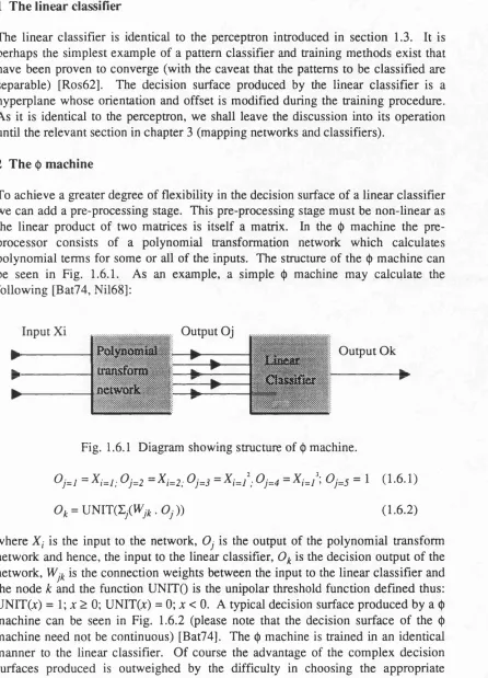
To achieve a greater degree of flexibility in the decision surface of a linear classifier we can add a pre-processing stage. This pre-processing stage must be non-linear as the linear product of two matrices is itself a matrix. In the 0 machine the pre processor consists of a polynomial transformation network which calculates polynomial terms for some or all of the inputs. The structure of the <j) machine can be seen in Fig. 1.6.1. As an example, a simple 0 machine may calculate the following [Bat74, Nil68]:
Output Oj
O utput Ok
i£l§£
Fig. 1.6.1 Diagram showing structure of 0 machine.
Or_, = X M ; Oj=2 = X M . Oh 3 = X M \ 0 M = X M \ Oh 5 = 1 (1.6.1)
Ok = UNIT(Ej(W;jt. Oj)) (1.6.2)
Fig. 1.6.2 Typical decision region created by a 0 machine.
1.6.3 The piece-wise linear classifier
To alleviate the need for a polynomial transformation network, we can realise the complex decision surfaces produced by the 0 machine by combining the outputs of a number of linear classifiers using either combinational circuitry or further stages of linear classifiers. In the case where layers of linear classifiers are used then this is identical to the multi-layer perceptron which we will again consider in detail in chapter 3.
1.6.4 The nearest neighbour classifier
An alternative technique to using the linear classifier is to create the decision surface by categorising an input to that of the nearest locate by using a nearest neighbour classifier (NNC). A locate is simply a point in the input state space that has been assigned a class. The locates can be generated in a number of ways. Perhaps the simplest technique is to use each training vector as a locate. On can reduce the storage overhead by removing those locates which do not contribute greatly to the form of the decision surface and algorithms exist for this [Bat74,78]. The decision surfaces produced by the NNC are piece-wise linear and can realise any surface given a sufficient quantity of appropriately positioned locates. It should be emphasised that the position of the locates does not necessarily infer anything about the patterns, the only function of the locates is to produce the decision surface.
1.6.5 The k nearest neighbour classifier
each of the stored locates. However where the k NNC differs is that the k nearest locates are considered and the class which has the democratic majority amongst the selected locates chosen [Bat74,78] and for this reason, k is normally odd to avoid "ties". As before, the decision surface produced is piece-wise linear (when a Euclidian distance metric is used) [Bat74]. The advantage that the k NNC (k > 1) has over the NNC is that the smoothing operation produced by taking the consensus of the k locates improves the decision surface by removing some of the "kinks" and hence can improve the generalisation [Bat74,78].
1.6.6 The c-means and fuzzy c-means clustering algorithms
A popular unsupervised clustering technique used in conventional pattern recognition is the c-means (alternatively known as the isodata or &-means) clustering algorithm [Har75]. In this technique, the data is individually "tagged" to one of the c clusters. Each application of the algorithm tests the data points in turn to see if moving the data to another cluster reduces the overall squared distance (using an appropriate distance metric). The data points to be reassigned are not normally relabelled until the entire data set has been examined. The algorithm is terminated when no further reduction in the squared distance can be obtained. An improvement on this technique utilises fuzzy set theory. The fuzzy c-means algorithm [Kan82] assigns a membership (a numerical value between 0 and 1) between each input and each cluster such that the total membership for any particular input to all clusters is equal to 1. The algorithm minimises the overall product of the membership (raised to a power, eg. 2) and the squared distance. In both the c-means and fuzzy c-means, we can assess which cluster a new input should belong by employing a ^-nearest neighbour strategy [Dud73,Bat74]. The disadvantage of using these techniques is that the data must be tagged and reapplied as "training" takes place and therefore they are only suitable for analysing a small (due to the large storage requirements) fixed data set [Lip87a] (eg the nutrition content of a range of foods [Har75]). Part of the impetus of neural network research is the ability to use training data that is non-repetitive and therefore cannot be tagged (eg. live speech) using only the storage required for the adjustable parameters. As with the Kohonen network, there is a superficial similarity between the c-means and fuzzy c-means algorithms and the training equations to be described in subsequent chapters and this similarity will be highlighted when they are introduced in chapter 2 [Koh88, Lip87a, Hou91a].
1.6.7 The compound and Gaussian classifiers
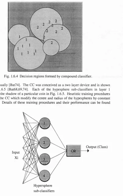
Fig. 1.6.4 Decision regions formed by compound classifier.
done manually [Bat74]. The CC was conceived as a two layer device and is shown in Fig. 1.6.5 [Bat68,69,74]. Each of the hypesphere sub-classifiers in layer 1 produces the shadow of a particular coin in Fig. 1.6.5. Heuristic training procedures exist for the CC which modify the centre and radius of the hypespheres by constant amounts. Details of these training procedures and their performance can be found
Input Xi
f :
ssssssssssss
Hypersphere sub-classifiers
Output (Class) ►
in [Bat74,78].
The maximum likelihood Gaussian classifier is also a two layer device except that the only function carried out by the second layer is to select the maximum output from the first layer [Dud73, Lip87a]. Essentially, the first layer of the consists of a series of multinormal Gaussian functions, one for each class. The mean and covariance of each distribution is calculated using maximum likelihood estimates. This strategy is successful if the underlying distribution of the input is also Gaussian. However, if the input distribution is not Gaussian, then the performance of the classifier will degrade [Lip87a] and this is particularly noticeable if the class to be recognised contains disjoint regions [Hua87]. Again there is a superficial similarity between the Gaussian classifier and the radial basis function (RBF) mapping network to be described in chapter 3. In this case however, the differences between the two schemes will manifest itself by the exemplary performance of the new RBF network when confronted with disjoint regions [Hou89b].
1.7 Outline of thesis, a simple model of perception
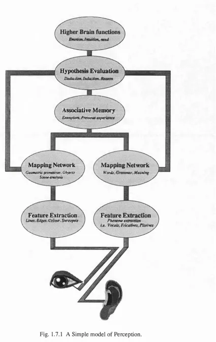
The categorisation of ANNs can be done in several ways. Lippmann based his excellent review on those networks that use either supervised or unsupervised training procedures and whether the network handles continuous or discrete (binary) signals [Lip87a]. In this thesis we shall adopt a different approach. We shall use a subjective, simple model of artificial perception, to relate the different ANN structures to their function. It must be stressed that this model is not intended to represent the functioning of the brain but instead encapsulates the building blocks necessary to design an artificial perceptual system. To aid in the understanding and application of the networks to be described, the simple model will refer to the processing that maybe carried out on visual and speech signals throughout each stage of perception. The flow diagram for this simple model can be seen in Fig. 1.7.1 and this figure should be referred to throughout this thesis.
Obviously, the first part of any model of perception is the input to the system. In the case of visual perception, this is the incoming light which is focused by the lens on to the back of the retina. In speech the sound input is in the form of pressure waves through the air. An artificial system can conceivably take any form of input, the only requirement being that a suitable transducer exists to convert the input into appropriate electrical signals (assuming an electronic implementation). Converting the electrical input in to a suitable signal for a network to utilise, is the first stage in the process of artificial perception and may be considered as pre-processing which we will consider in the next chapter. The remaining four stages in our simple perception are;
Emotion, imM&i.f&ed
Hypothesis Evaluation
Deduction, induction, Reason | |
Associative Memory
Bxmptm, Emkm ixpirkm*
Mapping Network
Geometric primatives. Objects V $4*M#wip4$
M apping Network Words, Gramtmrt Meaning
Feature Extraction::
Cttimtt, Steteopsis Feature ExtractionPhfiMiKexmcmn Mf, Vocals, Fricatives, ftostves
(2) Mapping
(3) Associative memory
(4) Hypothesis evaluation
The interelation of these four stages can be seen in Fig. 1.7.1. Chapters 2-5 cover these categories giving details of the major works and the contributions made by the author. Chapter 6 explores the possibility of unifying the architectures presented in chapters 2-5 and chapter 7 covers the electronic implementation of these systems using both analogue and digital techniques. Finally, chapter 8 summarises the conclusions from each of the previous chapters and looks to the future to assess what subjects within the umbrella of ANN research will come to the fore and suggests new avenues of research. In assessing the relative merits of the networks to be discussed, we shall base any conclusions on engineering efficiency (eg. the number of training cycles required to achieve a particular accuracy) and not how closely the network replicates the biological system for example. This stance results from the environment in which this work took place and not from any prejudice.
Before we embark on the first level of our perceptual system, we shall introduce the radial basis function (RBF) neuron. This device is the fundamental building block of the various structures to be described and appears in every chapter to follow. It is for this reason that we introduce it now.
1.8 An alternative to the first order model, the radial basis function
notation to be used throughout this thesis.
Ok = 'LjWjk .f(\\X r Wij\\) (1.8.1)
where Ok is the output of layer 2, W-, Wjk are the connection weights between layers 0, 1 and 1, 2 respectively, fQ is the activation function of layer 1 (eg Gaussian) and the symbols II II represent an appropriate distance metric (normally Euclidian). In Broomhead’s et al's implementation [Bro88], the RBF centres correspond to the data points. This leaves the weights Wjk to be assigned. As the output (0*) is linear with respect to these connections, their values can be determined directly by solving the set of linear equations formed, using matrix inversion [Bro88]. Using as many RBFs as data points, a global solution is guaranteed. However, in all but the simplest of problems, the parity between data points and RBFs would be impractical as the computational overhead would be excessive and hence the implementation would be problematic. Also, the results may be misleading as the interpolation surface will fit to inprecise or noisy data [Bro88]. These difficulties can be reduced by relaxing the link between the number of RBFs and data points and also relaxing the condition that the centres of the RBFs correspond to the location of the data points. In doing this however, the curve fitting problem becomes overspecified such that no unique inverse exists to calculate Wjk directly. Using the Moore- Penrose pseudo inverse in a minimum norm least squares method, we can carry out linear optimisation to determine Wjk [Bro88]. This technique will yield the optimum solution for the RBF centre points chosen but the solution will not be globally optimum (but will be locally optimum) as the quality of solution is heavily dependent on the location of the RBF centres which are chosen arbitrarily [Bou91]. Work has been done using an orthogonal least squares technique to decide which subset of data points should be chosen for the RBF centres and some success achieved [Che91]. However, the extra computations required may offset any benefits obtained. It is interesting to note that it is also possible to train the single layer perceptron using the afore mentioned linear optimisation procedure instead of the perceptron convergence procedure (PCP). In fact this technique was known before the PCP but the difficulty in inverting the large matrices produced made the development of simple training procedures attractive [Dud73]. However, although there are practical difficulties with Broomhead et al particular implementation, it has been applied with some success to speech pattern classification.
Inputs Xi
Output Oj Connection weights Wij
Fig. 1.8.1 Symbol used for RBF neuron.
trained using backpropagation [Hou89b]. Further, the network also measures the noise in the input data and can signal if an input occurs outside the error bounds found from the training data. The network can then give a "don't know" response in addition to it's "best guess" which is of considerable interest with applications that are safety critical. The symbol that we shall use for an RBF neuron (or node) can be seen in Fig. 1.8.1. The RBF that we shall use in this thesis can be expressed as follows:
netj= I.i WCr Wijp \ (1.8.2)
Oj = cxp(-Aj.netj) (1.8.3)
= exp (-netj/dj) (1.8.4)
where X { is the input to the network, is the connection weight which represents the centre of the Gaussian function of node y, netj is the total input to node y, Aj is a reciprocal measure of the radii (in each dimension) of influence and dj is a measure of the radii and is also the variance of the Gaussian function (i.e. aj~l = Aj). This defines an N dimension hypersphere. A hyperellipsoid, whose axes are aligned with each dimension, can be produced by replacing the Aj in eqn. 1.7.4 by as shown below:
netj= ^ [ A ^ - W ^ ] (1.8.5)
Oj = exp {-netj) (1.8.6)
1.9 Summary
In this chapter we have introduced the concept and motivation for ANNs. The intricacies of the biological neuron were considered and the difficulty in accurately modelling its characteristics discussed. A brief history of ANN research was then given and the simplified model of the neuron used in the majority of artificial systems shown. As the primary motive force for ANNs is pattern recognition, basic concepts were considered along with some of the most popular techniques which have emerged from the discipline. To categorise the networks to be described, a hypothetical model of perception was introduced. This model forms the skeleton of this thesis and is the framework to which we will refer the various networks to be covered in the chapters to follow. The five stages required for perception are:
(1) Self-organisation and Feature extraction.
(2) Mapping networks and classifiers.
(3) Associative memories.
(4) Hypothesis evaluation.
(5) Higher brain functions.
Self-organisation and feature extraction
Feature Extraction 1
• : Phoneme extr4Ctk>n p p
f a Vocoty Fricatives^ Plostm s
The first level in our simple model of perception is self-organising feature extraction and is one of the fundamental building blocks of our perceptual system. In infancy the brain is required to analyse and extract the important information from the complex signals arriving from the various senses without reference to an exemplar. In speech recognition for example, the post-natal infant will have no a priori knowledge of the language it is to learn, it must extract the phonemes of speech with no other reference than listening to the conversation of its elders. In visual recognition, feature extraction reduces the immense array of luminence values emerging from the receptor cells at the back of the eye to sets of primitives such as edges, surfaces, steriopsis etc. Essentially, a self-organising network must adapt itself in such a way so as to quantise the statistical distribution of the inputs within the input state space to reduce the immense amount of information entering the brain. By removing data which is in some sense redundant, the data processing carried out by the brain becomes tractable [Koh88a,b, Joh88, Barl90, Barr87, Lip87a, Trei84].
cortex (area 17) compare responses from neighbouring cells. If the fibre to which it is attached does not fire at the same time (on average) as those around it then it would seem likely that the fibre is misaligned. The cell will then cause the fibre to shrivel and die [Faw86]. This competitive self organising evolutionary behaviour (survival of the fittest) inherent in biological systems is reflected in the training strategies used in ANNs although the consequences are of course less severe. The two examples just given maybe thought of as the first stage in feature extraction. In speech recognition further stages will extract phonemes which are the basic building blocks of speech while in visual recognition lines, colour and perspective will be extracted from the perceived image. This reduction in data whilst retaining information and enhancing those properties required for perception characterise the role of a feature extractor. However, for a feature extractor to work successfully, we must present the data in the most suitable way. For example in speech recognition fine hairs in the cochlear act as a bank of tuned filters which approximate a one dimensional Fourier transform to supply the perceptual system with a measure of the incoming energy at different frequencies [Barr87]. We shall term this basic manipulation of the raw data as pre-processing which we will now consider briefly.
2.1 Pre-processing
Pre-processing in artificial systems is often carried out using circuits and techniques which are not based on a neural network approach. For this reason will shall not go into detail in this thesis on what techniques exist although it must be stressed that pre-processing is a vital part of any artificial pattern recognition or perceptual system and should be given due deference. However, for completeness, we shall briefly revue pre-processing in both the speech and visual systems in the brain as well as some artificial approaches.
2.1.1 Pre-processing in the speech and visual systems
Pre-processing in the speech and visual systems is carried out by the primary auditory and visual encoding components respectively. The primary auditory components are the ear, cochlea and auditory pathway. The outer ear acts as a pressure amplifier to the incoming sound waves. These sound waves vibrate the ear drum etc. (middle ear) which behaves as a mechanical transformer to convert fluctuations in air pressure to mechanical movement of the oval window in the cochlea. Rows of fine hairs within the inner ear (cochlea) convert pressure waves in the incompressible cochlea fluid caused by movement of the oval window membrane to frequency sensitive electrical signals. The signals are then carried away along the auditory pathway to enroute processing stations such as the superior olivery complex etc. and finally to the speech centres of the brain [Barr87, Joh88].