On the First Fall Degree of Summation Polynomials

(1)

POLYNOMIALS

STAVROS KOUSIDIS AND ANDREAS WIEMERS

Abstract. We improve on the first fall degree bound of polynomial

systems that arise from a Weil descent along Semaev’s summation poly-nomials relevant to the solution of the Elliptic Curve Discrete Logarithm Problem via Gr¨obner basis algorithms.

KEYWORDS. Polynomial systems, Gr¨obner bases, Discrete logarithm problem, Elliptic curve cryptosystem.

2010 MATHEMATICSSUBJECTCLASSIFICATION.13P15 Solving polyno-mial systems, 13P10 Gr¨obner bases, 14H52 Elliptic curves.

1. Introduction

Finding solutions to algebraic equations is a fundamental task. A common approach is a Gr¨obner basis computation via an algorithm such as Faug`ere’s

F4 andF5 (see [4, 5]). In recent applications Gr¨obner basis techniques have become relevant to the solution of the Elliptic Curve Discrete Logarithm Problem (ECDLP). Here one seeks solutions to polynomial equations arising from a Weil descent along Semaev’s summation polynomials [13] which represents a crucial step in an index calculus method for the ECDLP, see e.g. [12, 14]. The efficiency of Gr¨obner basis algorithms is governed by a so-called degree of regularity, that is the highest degree occurring along the subsequent computation of algebraic relations. It is widely believed that this often intractable complexity parameter is closely approximated by the degree of the first non-trivial algebraic relation, the first fall degree. In particular, the algorithms for the ECDLP of Petit and Quisquater [12] are sub-exponential under the assumption that this approximation is in o(1).

In the present paper, we will improve Petit’s and Quisquater’s [12] first fall degree boundm2+ 1 for the system arising from the Weil descent along Semaev’s (m+ 1)-th summation polynomial. That is, we prove that a degree

Federal Office for Information Security, Godesberger Allee 185–189, 53175 Bonn, Germany

E-mail address: [email protected].

Date: June 13, 2019.

2010 Mathematics Subject Classification. 13P15 Solving polynomial systems, 13P10 Gr¨obner bases, 14H52 Elliptic curves.

Key words and phrases. Polynomial systems, Gr¨obner bases, Discrete logarithm problem, Elliptic curve cryptosystem.

(2)

fall occurs at degreem2−m+1 by exhibiting the highest degree homogeneous part of that polynomial system. In fact, this degree is m2−m, so that we expect the bound to be sharp except for the somewhat pathological case

m= 2 that has been discussed by Kosters and Yeo [10]. This allows us to sharpen the asymptotic run time of the index calculus algorithm for the ECDLP as exhibited in the complexity analysis of Petit and Quisquater [12].

2. The first fall degree

The notion of the first fall has been described by Faug`ere and Joux [6, Section 5.1], Granboulan, Joux and Stern [7, Section 3], Dubois and Gama [3, Section 2.2], and Ding and Hodges [2, Section 3]. Although the concept of the first fall degree has been calledminimal degree [6] anddegree of regularity

[2, 3, 7], we actually adopt the terminology and definition of Hodges, Petit and Schlather [8]. For readability reasons we include a brief and tailored account of the first fall degree and refer the reader to [8, Section 2] for details and greater generality.

Our considerations take place over a degreen extensionF2n of the binary

fieldF2. Consider the decomposition of the graded ring

S=F2n[X0, . . . , XN−1]/(X02, . . . , X 2 N−1)

into its homogeneous components

S=S₀⊕S₁⊕ · · · ⊕S_N.

EachS_j is the F2n-vector space generated by the monomials of degreej. Let

I be an ideal in S generated by homogeneous polynomials h₁, . . . , h_r ∈S_d

all of the same degree d. Then we have a surjective map

φ: Sr −→ I

(g₁, . . . , g_r) 7→ g₁h₁+· · ·+g_rh_r.

Without loss of generality we furthermore assume 0< r= dim_F

2n

Pr

j=1F2nhj.

Lete_i denote the canonicali-th basis element of the freeS-module Sr. The

S-moduleU generated by the elements

hjei+hiej and hkek, wherei, j, k= 1, . . . , r,

is a subset of ker(φ). If we restrictφ to theF2n-subvector spaceS r

j−d⊂Sr

we obtain a surjective map

φj−d: Sj−dr −→ I ∩Sj

whose kernel contains the F2n-subvector spaceUj−d=U∩Sj−dr and hence

factors through

¯

φj−d:Sj−dr /Uj−d→I∩Sj.

Definition 2.1 (Cf. [8, Definition 2.1]). The first fall degree of a homoge-neous system h₁, . . . , h_r∈S_d and its linear span Pr

j=1F2nhj, respectively,

(3)

that is the smallestj such that dim_F

2n(I∩Sj)<dimF2n(S

r

j−d/Uj−d). It is

denoted by Df f( Pr

j=1F2nhj).

Following [8] we now consider the ring of functions

A_F

2n =F2

n[X₀, . . . , X_N−1]/(X₀2−X₀, . . . , X_N−12 −X_N−1) as a finite-dimensional filtered algebra whose filtration components [A_F

2n]d, d∈_N, are given by the polynomials up to degree d. The associated graded ring ofA_F

2n is

Gr(A_F

2n) =F2

n[X₀, . . . , X_N−1]/(X₀2, . . . , X_N2₋₁) whose graded components

[Gr(A_F

2n)]d= [AF2n]d/[AF2n]d−1, ford∈N,

are given by the homogeneous polynomials of degreed. Any linear subspace

V ⊂ [A_F

2n]d induces a homogeneous linear subspace ¯V ⊂ [Gr(AF2n)]d via

the canonical projection π_d: [A_F

2n]d→[Gr(AF2n)]d.

Definition 2.2 (Cf. [8, Definition 2.2]). Consider a polynomial system

p₁, . . . , p_r ∈[A_F

2n]d and its linear span V =

Pr

j=1F2npj ⊂[AF2n]d,

respec-tively. We assume without loss of generality that dim_F

2nV =r > 0. The

first fall degree ofV is

Df f(V) = (

d , dim_F

2n

¯

V <dim_F

2nV, Df f( ¯V) , else,

where D_{f f}( ¯V =Pr

j=1F2nπd(pj)) is given in Definition 2.1.

3. Weil descent along summation polynomials

We prove that the first fall degree of the polynomial system that arises from a Weil descent along Semaev’s summation polynomialS_m+1 is bounded from above bym2−m+ 1. This is an improvement overm2+ 1 that results from [8, Theorem 5.2] and [12, Section 4]. Let us briefly introduce the summation polynomials and describe the Weil descent.

Semaev [13] introduced them-th summation polynomialS_m(x₁, . . . , x_m)∈ K[x1, . . . , xm] on an elliptic curveE :y2=x3+a4x+a6 over a finite field

K with char(K) 6= 2,3 by the following defining property: for elements x₁, . . . , x_m in the algebraic closure ¯Kone hasSm(x1, . . . , xm) = 0 if and only

if there exist y1, . . . , ym ∈ K¯ such that (x1, y1), . . . ,(xm, ym) ∈ E( ¯K) and

(4)

E : y2 + xy = x3 +a₂x2 +a₆, and the projection to the x-coordinate

x(Pi) =x(xi, yi) =xi of Pi ∈E . Then, still

S₂(x₁, x₂) =x₁−x₂

and from Diem’s general description [1, Lemma 3.4, Lemma 3.5] one can deduce

S₃(x₁, x₂, x₃) = (x2₁+x2₂)x2₃+x₁x₂x₃+x2₁x2₂+a₆

Sm+1(x1. . . , xm, xm+1) = ResX(Sm(x1, . . . , xm−1, X), S3(xm, xm+1, X))

and the degree ofS_m+1in each variablex_i is 2m−1. Note that these formulas have also been outlined by Petit and Quisquater [12, Section 5] who also refer to Diem [1].

To describe the Weil descent along those summation polynomials (see e.g. [12, Section 4]) we fix a basis 1, z, . . . , zn−1 of F2n overF2 and letW be

a subvector space inF2n of dimension n 0

and basis ν1, . . . , ν_n0 over _F₂. We introduce mn0 variablesyij that model the linear constraints

xi= n0 X

l=1

yilνl,

set x_m+1 to an arbitrary elementc∈_F₂n, and obtain the equation system

S_m+1(x₁, . . . , x_m, c) =S_m+1



 n0 X

l=1

y_1lν_l, . . . ,

n0 X

l=1

y_mlν_l, c





=f₀(y_ij) +zf₁(y_ij) +· · ·+zn−1fn−1(yij)

The first fall degree of interest is that of the reduced polynomial system

s_k ≡f_kmod (y₁₁2 −y₁₁, . . . , y2_mn0−y

mn0), where k= 0, . . . , n−1.

(3.1)

Note thats₀, . . . , sn−1 ∈F2[y11, . . . , ymn0]/(y 2

11−y11, . . . , y 2

mn0−ymn0).

By the definition of the first fall degree we are interested in the highest degree homogeneous part of s0, . . . , sn−1 whose degree can be determined as

follows.

Lemma 3.1. Let m ≥ 3. The highest degree homogeneous part of the polynomial systems₀, . . . , sn−1∈F2[y11, . . . , ymn0]/(y

2

11−y11, . . . , y 2

mn0−ymn0)

from Equation 3.1 is induced by the monomial

(x₁· · ·x_m)2 m−1

−1_·

x_m+1

in the summation polynomial Sm+1(x1, . . . , xm, xm+1), and hence its degree

is less than or equal to m2−m.

Proof. First, we show the existence of the monomial (x₁· · ·x_m)2 m−1

−1_·

x_m+1

inSm+1(x1, . . . , xm, xm+1). We have

(5)

Sm+1(x1. . . , xm, xm+1) = ResX(Sm(x1, . . . , xm−1, X), S3(xm, xm+1, X))

and the degree of Sm+1 in each variable xi is 2 m−1

. The resultant of

f, g∈_F₂n[X] of degreek and lis the determinant of the Sylvester matrix Res_X(f, g) = det Syl(f, g)

= det



           

fk · · · f0

f_k · · · f₀

. .. . ..

f_k · · · f₀ g_l · · · g₀

g_l · · · g₀

. .. . ..

gl · · · g0 

           

That is, with

S₃(x_m, x_m+1, X) = (x2_m+x2_m+1)X2+x_mx_m+1X+x2_mx2_m+1+a₆ S_m(x₁, . . . , xm−1, X) =c₂m−2

,mX 2m−2

+· · ·+c_0,m

where each c_i,m∈_F₂n[x

1, . . . , xm−1], we have

S_m+1(x₁. . . , x_m, x_m+1) = det Syl(S_m, S₃)

.

To be concrete, Syl(S_m, S₃) is the matrix



      

c₂m−2

,m c2m−2−1,m · · · c0,m 0

0 c₂m−2

,m · · · c1,m c0,m

x2_m+x2_m+1 x_mx_m+1 x2_mx2_m+1+t

. .. . ..

x2_m+x2_m+1 x_mx_m+1 x2_mx2_m+1+t



      

with a total of 2m−2+ 2 rows and columns. In order to prove our claim we have to identify specific summands in the Leibniz formula of the determinant. That is, we consider

det Syl(Sm, S3)

=X

π

sgn(π)

2m−2+2 Y

i=1

Syl(Sm, S3)i,πi (3.2)

and argue that for the relevant summands no cancellation over F2n occurs.

Note that the sign of a permutation is 1∈_F₂n.

Step 1: Prove by induction (start with x2₁x2₂ in S₃) that S_m+1 contains the monomial (x1· · ·xm)2

m−1

in its term c0,m+1. For that we consider the

permutation

σ =

σ1, . . . , σ₂m−2

+2

(6)

=

2m−2+ 1,2m−2+ 2,1,2, . . . ,2m−2

and obtain

S_m+1(x₁. . . , x_m, x_m+1) = sgn(σ)

2m−2+2 Y

i=1

Syl(S_m, S₃)_i,σ_i +· · ·

=c_0,mc_0,m

2m−2 Y

i=1

(x2_m+x2_m+1) +. . .

=

(x1· · ·xm−1)2

m−22

·x2

m−1

m +. . .

= (x₁· · ·xm−1xm) 2m−1

+. . .

Note that specifyingσ₁= 2m−2+ 1 andσ₂= 2m−2+ 2 determinesσ since the remaining entries in Syl(Sm, S3) form an upper triangular matrix with

x2_m+x2_m+1 on the diagonal.

Step 2: Prove by induction (start withx₁x₂x₃ inS₃) thatS_m+1 contains the monomial (x₁· · ·x_m)2

m−1₋₁

·x_m+1, i.e. (x₁· · ·x_m)2 m−1₋₁

in its term c_1,m+1. For that we consider the permutation

τ =τ₁, . . . , τ₂m−2

+2

(3.4)

=2m−2,2m−2+ 2,1, . . . ,2m−2−1,2m−2+ 1 and obtain

S_m+1(x₁. . . , x_m, x_m+1)

= sgn(τ)

2m−2+2 Y

i=1

Syl(S_m, S₃)_i,τ i+· · ·

=c_1,mc_0,m·x_mx_m+1

2m−2−1 Y

i=1

(x2_m+x2_m+1) +. . .

= (x₁· · ·xm−1)2

m−2

−1_·

(x₁· · ·xm−1)2

m−2

·x_mx_m+1(x2_m)2 m−2

−1

+. . .

= (x₁· · ·xm−1xm)

2m−1−1_·

x_m+1+. . .

Note that specifying τ1 = 2 m−2

and τ2 = 2 m−2

+ 2 determines τ since the remaining entries in Syl(S_m, S₃) form an upper triangular matrix with

x2_m+x2_m+1, . . . , x_m2 +x2_m+1, x_mx_m+1 on the diagonal.

Second, in order to exclude potential cancellations we have to show that the permutations σ in (3.3) and τ in (3.4) are the only possible choices to produce the monomials (x₁· · ·x_m)2

m−1

and (x₁· · ·x_m)2 m−1₋₁

·x_m+1 in

(7)

that the only multiples of (x₁· · ·x_m)2 m−1₋₁

in the coefficients ofS_m+1 are (x₁· · ·x_m)2

m−1

in c_0,m+1 and (x₁· · ·x_m)2 m−1

−1

in c_1,m+1. Indeed, the factor (x₁· · ·xm−1)2

m−1₋₁

in the variables x₁, . . . , xm−1 can only be produced by

productsc_i,m·c_j,m of entries taken from the first two rows of the Sylvester matrix Syl(S_m, S₃). Since the degree of S_m in each variable x₁, . . . , xm−1

is 2m−2, each of the entries c_0,m, . . . , c₂m−2

,m is a sum of monomials in the

variablesx₁, . . . , xm−1 where each monomial is either

(i) no multiple of (x₁· · ·xm−1)2

m−2

−1

or

(ii) a multiple (x1· · ·xm−1)2

m−2

−1

·xδ1

1 · · ·x δm−1

m−1, withδi∈ {0,1}.

Therefore, the monomials in the products ci,m·cj,m that contribute to the

determinant (3.2) occur in the following forms

((x1· · ·xm−1)2

m−2

−1

)2·xδ1+δ

0

1

1 · · ·x δm−1+δ

0 m−1

m−1

(3.5)

(x₁· · ·xm−1)2

m−2₋₁ ·xδ1

1 · · ·x δm−1

m−1 ·µ

(3.6)

µ·µ0

(3.7)

where µandµ0 denote elements that are no multiples of (x₁· · ·xm−1)2

m−2

−1

. Consequently, a monomial in the productci,m·cj,m that is now a multiple of

(x₁· · ·xm−1)2

m−1

−1

can only arise in case (3.5) if for each k= 1, . . . , m−1 the following condition holds

2·2m−2−1

+δk+δ 0 k≥2

m−1

−1 ⇐⇒ δk+δ 0 k ≥1.

Due to the degree restriction ofS_m a productc_i,m·c_j,mwhere the monomials inc_i,m and c_j,m are all of the form (3.6) or (3.7) cannot produce a multiple of (x1· · ·xm−1)2

m−1

−1

. Therefore, we are left with products of the terms

c_0,m andc_1,m by the induction hypothesis. Sincec_1,m·c_1,m only produces (x1· · ·xm−1)2

m−1

−2

, the permutationsπ = (π1, π2, . . . , π₂m−2

+2) in the

Leib-niz formula (3.2) that produce multiples of the monomial (x₁· · ·xm−1)2

m−1

−1

must have either (π1, π2) = (σ1, σ2) or (π1, π2) = (τ1, τ2) as given in (3.3) and

(3.4), respectively. This determines our permutationsσ and τ completely. To finish the proof, our degree claim in Lemma 3.1 is argued as follows. The variables y_ij of the s_k are over F2 where taking squares is a linear

operation. Therefore the degrees of the homogeneous parts of the system

s₀, . . . , sn−1depend only on the Hamming weight wt(xα11· · ·x αm

m ) = P

wt(α_i) of a monomial inS_m+1. Since the degree ofS_m+1 in each variable x_i is 2m−1 the monomial (x₁· · ·x_m)2

m−1

−1

·x_m+1, when x_m+1 is set to an elementc∈ F2n, produces the highest Hamming weight

Pm i=1wt(2

m−1

(8)

To be precise, we consider

x2

j

i = ( n0 X

l=1

y_ilν_l)2 j

=

n0 X

l=1

y_ilν2

j

l

and obtain

(3.8) (x₁· · ·x_m)2 m−1

−1_·

c=c

m Y i=1 m−2 Y j=0 n0 X l=1

y_ilν2

j

l

which is of degree less than or equal to m(m−1) in the variablesy_ij. We are ready to prove the main result.

Theorem 3.2. Let n0 ≥ m ≥3 and c∈ _F₂n \ {0}, and consider the

poly-nomial system s₀, . . . , sn−1 ∈ F2[y11, . . . , ymn0]/(y 2

11−y11, . . . , y 2

mn0 −ymn0)

from Equation 3.1, that results from the Weil descent along the summation polynomial S_m+1(x₁, . . . , x_m, c). The first fall degree of s₀, . . . , sn−1 is less

than or equal tom2−m+ 1.

Proof. Consider the finite-dimensional filtered algebra

A_F

2 =F2[y11, . . . , ymn0]/(y

2

11−y11, . . . , y 2

mn0−ymn0).

The linear span

n−1 X

j=0

F2sj

is inside the degree d=m2−m subspace of the filtered algebra A_F₂ due to Lemma 3.1. By [8, Corollary 2.4] an extension of the base field, i.e.

A_F

2n =F2

n[y₁₁, . . . , y

mn0]/(y 2

11−y11, . . . , y_mn2 0 −y

mn0),

does not affect the first fall degree. That is,

Df f 

 n−1 X

j=0

F2sj 

=D_{f f} 

 n−1 X

j=0

F2nsj 

.

By [8, Definition 2.2], the first fall degree of the subspace Pn−1

j=0F2nsj of

A_F 2n is

D_{f f}



 n−1 X

j=0

F2nsj 

= (

d=m2−m , dim_F

2n

¯

V <dim_F

2nV, D_{f f}( ¯V) , else,

where ¯V denotes the induced homogeneous subspace ofPn−1

j=0F2nsj in the

associated graded ring

Gr(A_F

2n) =F2

n[y

11, . . . , ymn0]/(y 2

(9)

If dim_F

2n

¯

V < dim_F

2nV, our claim follows. Otherwise we consider the

polynomial

P₀ =c

m Y i=1 m−2 Y j=0 n0 X l=1

y_ilν2

j

l

which is an element of the homogeneous subspace ¯V by Lemma 3.1, and in particular Equation 3.8. Now, for any

xk= n0 X

l=1

yklνl

we have a non-trivial relation

x_kP₀ =c

n0 X

l=1

y2_klν_l2·

m−2 Y j=1 n0 X l=1

y_klν2

j l · m Y i=1,i6=k m−2 Y j=0 n0 X l=1

y_ilν2

j

l = 0∈Gr(AF₂n)

of degree d+ 1 = m2 −m+ 1 unless P₀ = 0 ∈ Gr(A_F

2n). Therefore it

remains to show that P₀ 6= 0. For that purpose, we recall thatc∈_F₂n\ {0},

v₁, . . . , v_n0 are linearly independent, and n0≥m. Consider the linear change of variables

Yij =x2

j

i = ( n0 X

l=1

yilνl)2

j =

n0 X

l=1

yilν2

j

l .

This is induced by the m×n0 matrix

       

ν₁ · · · ν_n0

ν₁2 · · · ν_n20 ..

. . .. ...

ν2

m−2

1 · · · ν2

m−2

n0        

that can be completed to an invertible linear transform by [11, Lemma 3.51], since we have assumed v₁, . . . , v_n0 to be linearly independent and n0 ≥m. By using such an invertible linear transform on any block of variables

y_i1, . . . , y_in0 we get new variables

Y10, . . . , Y_m,n0

−1.

Under this change of variablesP₀ is mapped to the non-zero element

c m Y i=1 m−2 Y j=0

Yij ∈F2n[Y10, . . . , Y_m,n0

−1]/(Y 2

10, . . . , Y_m,n2 0

(10)

Remark 3.3. Our Theorem 3.2 remains true also in the case m= 2 with first fall degree less than or equal to 2·1 + 1 = 3. This bound is not sharp though, in fact the first fall degree in the case m= 2 equals 2 [10, Corollary 4.11 and Remark 4.12].

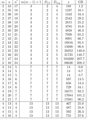
Table 1. Empirical data for the Weil descent along the summation polynomial Sm+1 over F2n with n

0

-dimensional factor basis. Displayed are the observed first fall degreeD_{f f}, degree of regularity Dreg, the time in seconds s and space

requirement in gigabyte GB. All values are averaged over 10 repetitions. For the casem= 2 see also Remark 3.3.

m n n0 m(m−1) + 1 D_{f f} D_reg s GB

2 34 17 3 2 4 188 1.2

2 35 18 3 2 4 1237 16.1

2 36 18 3 2 4 1342 16.4

2 37 19 3 2 5 2542 29.2

2 38 19 3 2 5 2815 25.2

2 39 20 3 2 5 4785 45.6

2 40 20 3 2 5 4858 46.3

2 41 21 3 2 5 7930 65.3

2 42 21 3 2 5 8901 66.7

2 43 22 3 2 5 16816 95.5

2 44 22 3 2 5 15690 96.8

2 45 23 3 2 5 38352 140.0

2 46 23 3 2 5 31735 140.7

2 47 24 3 2 5 103200 207.7

2 48 24 3 2 5 86636 208.2

3 13 5 7 7 7 14 0.6

3 14 5 7 7 7 14 0.7

3 15 5 7 7 7 14 0.7

3 16 6 7 7 7 597 13.5

3 17 6 7 7 7 656 13.3

3 18 6 7 7 7 729 34.1

3 19 7 7 7 7 16571 92.2

3 20 7 7 7 7 17684 101.2

3 21 7 7 7 7 17681 90.2

4 13 4 13 13 13 467 25.0

4 14 4 13 13 13 487 25.8

4 15 4 13 13 13 592 26.3

(11)

4. Experiments and Conclusion

In the light of the first fall degree bound given in Theorem 3.2 we computed a Gr¨obner basis for the ideal resulting from the Weil descent along the summation polynomialSm+1(x1, . . . , xm, xm+1) form= 2,3,4 on an AMD

Opteron CPU with Magma’sGroebnerBasis() function. Again, we set the verbose level to 1 and extracted the empirical first fall degree Df f as the

step degree of the first step where new lower degree (i.e. less than step degree) polynomials are added. The empirical degree of regularityDreg is

the highest step degree that appears during the Gr¨obner basis computation. In each experiment we chose a random non-singular elliptic curve overF2n, a

random subvector space of dimensionn0 =dn/meas the factor basis, and set

xm+1 to thex-coordinate of a random point on the curve. The experimental

results that extend the ones present in the literature by Petit and Quisquater [12] and Kosters and Yeo [10] are displayed in Table 1.

Like Kosters and Yeo [10, Section 5] we observed a raise in the regularity degree form= 2 in our experiments and were able to verify their observation that with the low degree polynomialsW = span{1, z, . . . , zn

0

} chosen as the factor basis (Cf. [14, Section 4.5]) the raise in the regularity degree was produced for slightly greatern= 45. It would be very interesting to observe a raise in the degree of regularity for higher Semaev polynomials, but time and memory amounts become a serious issue for m ≥ 3. However, such observations might neither falsify [12, Assumption 2] thatDreg =Df f+ o(1)

nor lead to further evidence that the gap between the degree of regularity and the first fall degree depends onn as discussed in [9, Section 5.2].

However, we believe our first fall degree bound m2−m+ 1 for Semaev polynomials to be sharp form≥3, and rephrase [12, Assumption 2] as the following question:

D_reg =m2−m+ 1 + o(1) ? (4.1)

Note that our upper bound on the first fall degree of summation polynomials is a first step towards answering this question. The first fall degree generically bounds the degree of regularity from below. Hence, any further lower bound on the degree of regularity associated to the specific case of a Weil descent along summation polynomials can potentially answer (4.1).

(12)

logarithm can asymptotically be solved in sub-exponential time

O

2clog(n)

n2/3+1

,

(4.2)

where c= 2ω/3,ω is the linear algebra constant (ω= log(7)/log(2) is used in the following estimates), andn2/3+ 1 is an upper bound for the first fall degree of them-th summation polynomial whenm=n1/3 [12, Proposition 1]. They state that, by following this analysis the index calculus approach beats generic algorithms with run timeO(2n/2) for anyn≥N whereN is an integer approximately equal to 2000. Now, based on Theorem 3.2 we assume D_reg ≈m2−m+ 1 =n2/3−n1/3+ 1 and sharpen (4.2) to

O

2clog(n)

n2/3−n1/3+1

.

(4.3)

Hence, the turning point to solve the ECDLP faster than a generic algorithm is an integer approximately equal to 1250. Note that this is still far from cryptographically relevant sizes ofnup to 521.

References

1. Claus Diem,On the discrete logarithm problem in elliptic curves, Compositio Mathe-matica147(2011), no. 1, 75–104.

2. Jintai Ding and Timothy J. Hodges,Inverting HFE systems is quasi-polynomial for all fields, CRYPTO, 2011, pp. 724–742.

3. Vivien Dubois and Nicolas Gama, The degree of regularity of HFE systems, ASI-ACRYPT, 2010, pp. 557–576.

4. Jean-Charles Faug`ere,A new efficient algorithm for computing Gr¨obner bases (F4), Journal of Pure and Applied Algebra139(1999), no. 1–3, 61–88.

5. Jean-Charles Faug`ere,A new efficient algorithm for computing Gr¨obner bases without reduction to zero (F5), Proceedings of the 2002 International Symposium on Symbolic and Algebraic Computation, ISSAC ’02, 2002, pp. 75–83.

6. Jean-Charles Faug`ere and Antoine Joux,Algebraic cryptanalysis of hidden field equation (HFE) cryptosystems using Gr¨obner bases, CRYPTO, 2003, pp. 44–60.

7. Louis Granboulan, Antoine Joux, and Jacques Stern,Inverting HFE is quasipolynomial, CRYPTO, 2006, pp. 345–356.

8. Timothy J. Hodges, Christophe Petit, and Jacob Schlather,First fall degree and Weil descent, Finite Fields and Their Applications30(2014), 155–177.

9. Ming-Deh Huang, Michiel Kosters, and Sze Ling Yeo,Last fall degree, HFE, and Weil descent attacks on ECDLP, CRYPTO, 2015, pp. 581–600.

10. Michiel Kosters and Sze Ling Yeo,Notes on summation polynomials, Preprinthttp: //arxiv.org/abs/1505.02532(2015).

11. Rudolf Lidl and Harald Niederreiter,Introduction to finite fields and their applications, Cambridge University Press, New York, NY, USA, 1986.

12. Christophe Petit and Jean-Jacques Quisquater,On polynomial systems arising from a Weil descent, ASIACRYPT, 2012, pp. 451–466.

13. Igor Semaev,Summation polynomials and the discrete logarithm problem on elliptic curves, IACR Cryptology ePrint Archive2004(2004), 31.

14. ,New algorithm for the discrete logarithm problem on elliptic curves, Preprint