Self-Consistency In Sequential Decision-Making

(1)

University of Pennsylvania

ScholarlyCommons

Publicly Accessible Penn Dissertations

2018

Self-Consistency In Sequential Decision-Making

Long Luu

University of Pennsylvania, [email protected]

Follow this and additional works at:

https://repository.upenn.edu/edissertations

Part of the

Neuroscience and Neurobiology Commons, and the

Psychology Commons

This paper is posted at ScholarlyCommons.https://repository.upenn.edu/edissertations/3152

Recommended Citation

Luu, Long, "Self-Consistency In Sequential Decision-Making" (2018).Publicly Accessible Penn Dissertations. 3152.

(2)

Self-Consistency In Sequential Decision-Making

Abstract

Human decisions are rarely made in isolation. We typically have to make a sequence of decisions to reach a goal. Studies in economics and cognitive psychology have shown that making a decision may result in several biases in subsequent judgments. Similar biases have also recently been found in human percepts of low-level stimuli such as motion direction. What lacking is a principled framework that can account for several sequential dependencies between judgments. Towards that goal, in my thesis, I propose and experimentally test a self-consistent Bayesian observer model that assumes humans maintain self-consistency along the inference process. In Chapter 2, I first demonstrate that after having made a categorical decision on stimulus orientation, subjects’ estimate of the stimulus is systematically biased away from the decision boundary. Two additional experiments suggest that the bias occurs because subjects treat their first decision as a fact and use that to constrain the subsequent estimation. Model fit to the data in my experiments and data in previous studies show that the self-consistent Bayesian model can quantitatively account for human behaviors in a wide range of experimental settings. In Chapter 3, using the same decision-estimation tasks, I probed the post-decision sensory representation by providing feedback on the categorical post-decision. I found that subjects’ sensory representation is kept intact and the self-consistency is implemented by conditioning the prior distribution on the categorical decision. The results also suggest another interesting form of self-consistency when subjects’ decision was incorrect: they reconstructed the sensory measurement to make it consistent with the given feedback. In Chapter 4, I found that the choice-induced bias also occurs in human judgment of number. The bias is similar for both non-symbolic (cloud of dots) and symbolic (sequence of Arabic

numerals) forms of number. Finally, I propose in the general discussion how the self-consistent Bayesian framework may account for other biases in sequential decision-making such as the halo effect and sunk-cost fallacy.

Degree Type

Dissertation

Degree Name

Doctor of Philosophy (PhD)

Graduate Group

Psychology

First Advisor

Alan A. Stocker

Keywords

Bayesian decision theory, Decision-making, Perception, Psychophysics, Self-consistency, Sequential judgment

Subject Categories

(3)

SELF-CONSISTENCY IN SEQUENTIAL DECISION-MAKING

Long Luu

A DISSERTATION

in

Psychology

Presented to the Faculties of the University of Pennsylvania

in

Partial Fulfillment of the Requirements for the

Degree of Doctor of Philosophy

2018

Supervisor of Dissertation

Alan A. Stocker, Associate Professor of Psychology

Graduate Group Chairperson

Sara Jaffee, Professor of Psychology

Dissertation Committee

David H. Brainard, Professor of Psychology Joshua I. Gold, Professor of Neuroscience

(4)

Dedicated to my parents and my wife

(5)

Acknowledgment

I would like to express my gratitude to many people who have helped to bring this thesis

to fruition.

First I want to thank my advisor, Alan Stocker, for his dedicated mentoring. I have

learned from him how to become a proper scientist which ranges from doing solid science and

efficiently communicating my works to the scientific community to developing a scientific

career. In every aspect of the scientific enterprise, Alan has shown me the high standards I

should always aspire to.

I am also deeply grateful to my thesis committee, David Brainard, Josh Gold and Joe

Kable for their relentless support and helpful guidance during my PhD years. I want to

especially thank David for introducing me to the beauty and fascination of vision science

and psychophysics. I want to thank Josh for always giving constructive feedback and helping

me see the problem from a different perspective. I am grateful to Joe for his willingness to

help when I need it.

I am grateful to many people in Psychology Department. First I would like to thank the

administrative staffs, especially Yuni Thornton, Laurel Sweeney and Jessica Marcus who

have helped me a lot with the administrative works. I also want to thank many faculty

members in psychology who have introduced me to the exciting field of psychology through

proseminar courses.

During the years at Penn, I have received generous mentoring and enjoyed friendship

with many fellow students and postdocs, especially those in perception group. Manuel

Spitschan provided me with detailed and valuable guidance in performing psychophysical

experiment. Xuexin Wei always gave me interesting insights in our frequent conversation

both inside and outside the lab. I want to thank Ana Radonjic, Nicolas Cottaris, Toni

Sareela, Matjaz Jogan, Pedro Ortega, Alan He, Mohammad Rostami, Daniel Pak,

Ben-jamin Chin, Cheng Qiu, Jiang Mao, Lingqi Zhang, Noam Roth, David White, Michael

Barnett, Yunshu Fan and Takahiro Doi for many interesting discussions and conversations

(6)

Last but not least, I want to thank my parents, my uncle Vuong and my wife for their

relentless and unconditional support for my professional career no matter what path I have

(7)

ABSTRACT

SELF-CONSISTENCY IN SEQUENTIAL DECISION-MAKING

Long Luu

Alan A. Stocker

Human decisions are rarely made in isolation. We typically have to make a sequence of

decisions to reach a goal. Studies in economics and cognitive psychology have shown that

making a decision may result in several biases in subsequent judgments. Similar biases have

also recently been found in human percepts of low-level stimuli such as motion direction.

What lacking is a principled framework that can account for several sequential

dependen-cies between judgments. Towards that goal, in my thesis, I propose and experimentally test

a self-consistent Bayesian observer model that assumes humans maintain self-consistency

along the inference process. In Chapter 2, I first demonstrate that after having made a

categorical decision on stimulus orientation, subjects’ estimate of the stimulus is

systemat-ically biased away from the decision boundary. Two additional experiments suggest that

the bias occurs because subjects treat their first decision as a fact and use that to constrain

the subsequent estimation. Model fit to the data in my experiments and data in previous

studies show that the self-consistent Bayesian model can quantitatively account for human

behaviors in a wide range of experimental settings. In Chapter 3, using the same

decision-estimation tasks, I probed the post-decision sensory representation by providing feedback

on the categorical decision. I found that subjects’ sensory representation is kept intact and

the self-consistency is implemented by conditioning the prior distribution on the categorical

decision. The results also suggest another interesting form of self-consistency when subjects’

decision was incorrect: they reconstructed the sensory measurement to make it consistent

with the given feedback. In Chapter 4, I found that the choice-induced bias also occurs

in human judgment of number. The bias is similar for both non-symbolic (cloud of dots)

and symbolic (sequence of Arabic numerals) forms of number. Finally, I propose in the

general discussion how the self-consistent Bayesian framework may account for other biases

(8)

List of figures

Figure 1.1: Example to illustrate Bayesian decision theory . . . 14

Figure 2.1: Post-decision biases in a perceptual task sequence . . . 17

Figure 2.2: Bayesian observer models for the perceptual task sequence . . . 19

Figure 2.3: The self-consistent Bayesian observer model . . . 21

Figure 2.4: Experiment 1: Data and model fits for individual subjects . . . 22

Figure 2.5: Effect of the stimulus prior . . . 24

Figure 2.6: Self-made vs. given category assignment . . . 25

Figure 2.7: Experiments 2 and 3: Joint fit to data for individual subjects . . . . 27

Figure 2.8: Inconsistent trials are due to lapses and motor noise . . . 29

Figure 2.9: Model fits for experimental data by Zamboni et al. (2016) . . . 31

Figure 2.10: Maintaining self-consistency in the face of working memory noise . . 34

Figure 2.11: Full distributions of individual subjects’ estimates in Experiment 1 . 47 Figure 2.12: Measured motor noise of individual subjects . . . 48

Figure 2.13: Histogram plots of the orientation estimates together with the model fit for Experiment 1 (combined subject) . . . 49

Figure 2.14: Goodness-of-fits for Experiment 1 . . . 50

Figure 2.15: Full distributions of individual subjects’ estimates in Experiment 2 . 51 Figure 2.16: Full distributions of individual subjects’ estimates in Experiment 3 . 52 Figure 2.17: Goodness-of-fits for Experiments 2 and 3 . . . 53

Figure 2.18: Zamboni et al. (2016) data (Experiment 1, combined subject) and fit with the self-consistent observer model . . . 54

Figure 2.19: Zamboni et al. (2016) data (Experiment 2, combined subject) and fit with the self-consistent observer model . . . 55

(12)

Figure 3.1: Alternative hypotheses of post-decision sensory representation. . . . 59

Figure 3.2: Prediction of alternative hypotheses for incorrect trials. . . 60

Figure 3.3: Self-consistent model fit to correct trials. . . 62

Figure 3.4: Data and model prediction for incorrect trials. . . 63

Figure 3.5: Performance of alternative models in Experiment 1. . . 65

Figure 3.6: Dissociating the models by imposing an asymmetric prior. . . 66

Figure 3.7: Model prediction and data in Experiment 2. . . 67

Figure 3.8: Performance of alternative models in Experiment 2. . . 69

Figure 4.1: Experiment 1 procedure . . . 80

Figure 4.2: Data and model fit in Experiment 1 . . . 82

Figure 4.3: Experiment 2 procedure and result . . . 85

Figure 4.4: Comparing alternative models . . . 86

Figure 4.5: Instruction for Experiment 3 . . . 88

Figure 4.6: Experiment 3 result . . . 90

Figure 4.7: Histogram of subjects’ estimates and model fits in Experiment 1 . . 98

Figure 4.8: Correlation of sample position and decision . . . 99

Figure 5.1: Rational Bayesian observer of multi-attribute judgment . . . 104

Figure 5.2: Self-consistent observer of multi-attribute judgment . . . 105

Figure 5.3: Experimental test of halo effect at low-level perception . . . 106

Figure 5.4: Modeling sunk cost fallacy . . . 110

Figure 5.5: Advantage of self-consistent Bayesian observer . . . 111

(13)

Chapter 1 Introduction

As the field of machine intelligence advances at a blistering pace, we are now used to

hearing breaking news about machine beating human experts on many areas once thought

to be exclusively for the human. That ranges from AlphaGo beating Go champions (Silver

et al., 2016, 2017), machine learning algorithms making medical decisions (Obermeyer and

Emanuel, 2016; Kononenko, 2001) to autonomous robots fighting in wars (Singer, 2010;

Ayoub and Payne, 2016). It leaves many of us to wonder what will be left for human

intelligence. A common response is that we are still far from building a machine that makes

a medical diagnosis in the morning, then drives to a friend’s home to play a chess game in

the afternoon and is ready to get in war at any time if necessary. In other words, the best

machines excel humans at a specific area yet fall far behind an average person in all other

areas (Lake et al., 2017; Kasparov, 2017).

Among areas that machines are still behind human in many regards is perception which

involves judgments about basic properties of the world. Deep Blue computer that defeated

Gary Kasparov cannot tell whether the sky is blue or how deep the ocean is. The ease

with which we make such perceptual decisions conceals the complexity of the underlying

processes. For instance, driving appears to be a fairly basic skill for most people, yet it

requires a tremendous amount of complicated decisions many of which involve inference

about perceptual features of the world (e.g. what are the surrounding objects and how far

away or how fast are they?). The challenges are more obvious with the development of

state-of-the-art technologies such as self-driving cars or humanoid robots. In fact, research on

perception dates back to as early as the 19thcentury when the pioneers like Gustav Fechner

and Hermann von Helmholtz conceived the lawful relations between the mental process and

(14)

works has followed those early attempts and greatly advanced our understanding of how

humans perceive the world (Cornsweet, 2012; Blakemore, 1993; Wandell, 1995; Green and

Swets, 1966; Wolfe et al., 2006). In these studies, human subjects typically make a single

judgment on a simple stimulus in each trial (see Supplemental-psychophysics methods for a

brief overview of experimental methods). Crucially, the dominant theoretical frameworks in

perception such as linear system theory (Wandell, 1995), signal detection theory (Macmillan

and Creelman, 2004) and Bayesian decision theory (Kersten and Schrater, 2002; Maloney,

2002) mostly assume that perceptual judgments are made independent of each other. As a

result, a perceptual decision should not affect subsequent judgments.

However, several lines of research in cognition and perception suggest that there exist

many forms of sequential dependency between decisions. In cognitive psychology and

eco-nomics, a rich body of works found evidence that a decision may cause systematic biases

in subsequent judgments (Abelson, 1968; Kahneman, 2011). For instance, when humans

made a sequence of judgments on the same stimulus features, the later judgment tend to

be distorted to be consistent with the preceding decision (Brehm, 1956). Several other

decisional biases induced by preceding judgments have also been well documented such as

confirmation bias (Nickerson, 1998), halo effect (Nisbett and Wilson, 1977) and sunk-cost

fallacy (Arkes and Blumer, 1985).

Several perception studies have found that perceptual decisions across trials exhibit

specific patterns such as repetition or alternation despite the fact that the experimental

stimuli were randomized (Fernberger, 1920; Gold et al., 2008; Fr¨und et al., 2014). An

important difference between these studies and the cognitive literature mentioned above is

that subjects only made one decision in each trial, which makes it difficult to have a direct

comparison. More recently, a small body of works in perception had multiple judgments in

each trial and show biases that are similar to the cognitive biases (Jazayeri and Movshon,

2007; Zamboni et al., 2016; Bronfman et al., 2015). As an example, a study by Jazayeri

and Movshon (2007) shows that after having made a decision on motion direction of a dot

(15)

from the decision boundary.

Although there exist many ad hoc theories that can explain each of these bias effects,

what we lack is a unifying model framework that may account for many of the findings

and provide fruitful predictions for future research. Towards that goal, my thesis extends a

self-conditioned Bayesian observer model (Stocker and Simoncelli, 2007) and demonstrates

through several experiments how the model can quantitatively account for sequential

de-pendency in human perceptual decisions across various experimental settings.

In the rest of the chapter, I provide the necessary background for the readers that are

not familiar with the relevant literature. Specifically, I will review key studies that show

several forms of sequential dependency between decisions in cognition and perception. Then

I will review the standard framework of Bayesian decision theory as applied in perception.

1.1. Sequential dependency in cognitive judgments

In 1956, the psychologist Leon Festinger published a book to describe the behavior of

mem-bers in a religious cult that believes the world would be destroyed by a flood on December

21, 1954 and the believers would be saved by a flying saucer (Festinger et al., 1956).

In-terestingly, after they found out that the end of the world did not happen, they readily

accepted the leader’ argument that the world is saved by their extreme piety and even

doubled down on their belief and fervently proselytized for it. To explain the phenomenon,

Festinger developed a theory of cognitive dissonance which posits that people dislike

holding contradictory beliefs in mind and tend to modify them to maintain a sense of

con-sistency (Festinger, 1957). In the religious cult example, the members’ belief that the world

would be destroyed is highly dissonant with the belief that the event did not happen.

Im-portantly, they cannot change either of them because they had given up everything (jobs,

spouses, possessions) to follow the cult. Therefore, they easily fell prey to demagoguery

claims and actively advanced those arguments that may help in reconciling these dissonant

beliefs.

Following on Festinger’s pioneering works, a large body of experimental studies has

(16)

and Carlsmith, 1959; Bem, 1972; Knox and Inkster, 1968; Younger et al., 1977; Frenkel and

Doob, 1976; Cohen and Goldberg, 1970). In a study by Brehm (1956) subjects were asked

to rate the desirability of eight items (e.g. coffee-maker, toaster, stopwatch). Then they had

to choose between two equally desirable options (e.g. coffee-maker vs. toaster) and rate the

items again. In accordance with cognitive dissonance theory, subjects’ ratings of the items

after a difficult decision change according to their choice, that is, the value of chosen item

increases whereas the value of rejected item decreases. This line of works has been revived

recently (Lee and Schwarz, 2010) and researchers recast it as choice-induced preference

(Egan et al., 2010; Sharot et al., 2010, 2012) or preservation of coherence/consistency (Simon

et al., 2004; Riefer et al., 2017). By using choice-blindness paradigm (Johansson et al., 2005),

the studies on choice-induced preference confirm that cognitive dissonance effect is not due

to statistical artifacts as pointed out by Chen and Risen (2010).

As reviewed above, cognitive dissonance studies demonstrate sequential dependency

between judgments that subjects make on the same feature using the same evidence.

How-ever, the practical situation that a decision maker encounters often involves judgments on

different attributes (e.g. intelligence, experience, and integrity of a job candidate). If the

judgments are made sequentially, the order in which the attributes are considered may

sig-nificantly affect the judgment results as demonstrated in studies on halo effect (Nisbett

and Wilson, 1977; Thorndike, 1920; Sigall and Ostrove, 1975; Leuthesser et al., 1995).

An-other typical real-life scenario is when we cannot acquire all relevant information at once.

Hence, we first make a preliminary decision and subsequently incorporate any additional

in-formation presented to us. For example, a company decides to invest in a promising project

with an initial estimated budget of $100 million dollars. Halfway through the project, all

money is spent and it is estimated that another $100 million dollars are needed to finish

it. Moreover, the project is not as promising as it was and the same amount of money can

be spent on another more profitable project. What should the company do? Anecdotal

observation and empirical evidence have shown that the company is more likely to continue

(17)

likely invest in the new project. This phenomenon is namedsunk-cost fallacy (Arkes and

Blumer, 1985; Staw, 1976). A related ”irrational” behavior, confirmation bias, was also well

documented in several studies which suggest that subjects tend to search for information

supporting their previous decision (Nickerson, 1998; Mynatt et al., 1977; Jonas et al., 2001).

Those scenarios will be discussed more extensively in section 5.2.

1.2. Sequential dependency in perceptual judgments

1.2.1. Single-judgment task

Even in the standard psychophysics experiments that include a single decision in a trial,

researchers have long noticed some dependency in subjects’ decisions across trials. As early

as 1920, Fernberger (1920) found that when subjects made a simple discrimination on a pair

of weights (”lighter”, ”heavier” or ”equal”), their decision in the current trial was repulsed

away from the decision in the previous trial (e.g. they tended to respond ”lighter” when

the response had been ”heavier” in the preceding trial). Several subsequent studies using

a wide range of stimuli and task designs found mixed results. In some studies, subjects

tended to avoid the previous response (Arons and Irwin, 1932; Preston, 1936; Collier, 1951)

whereas other studies show that subjects tended to repeat the previous response (Senders

and Sowards, 1952; Senders, 1953; Verplanck et al., 1952; Day, 1956; McGill, 1957). Several

studies have tried to determine the factors that influence this dependency such as training

(Verplanck et al., 1953), intertrial interval, experimental duration (Collier, 1954; Day, 1957)

and previous stimulus identity (Verplanck and Blough, 1958; Collier and Verplanck, 1958).

More recent studies replicated the sequential dependency and demonstrated that the effect

cannot be explained by motor bias, sensory adaptation or attentional effect (Akaishi et al.,

2014; Fr¨und et al., 2014; Braun et al., 2018). When feedback was given in every trial,

subjects’ decision is dependent on the feedback in the previous trial: repetition if correct

and alternation if incorrect (win-stay, lose-switch) (Busse et al., 2011; Abrahamyan et al.,

2016; Urai et al., 2017).

How can we explain this type of sequential dependency? Some proposed that the

(18)

a pattern even when the stimulus is totally ambiguous (Tune, 1964; Goodfellow, 1938).

Other researchers approached the problem from the perspective of signal detection theory

and suggested that the dependency occurs because the observer’s decision criterion

sys-tematically fluctuates throughout the experiment (Treisman and Williams, 1984; Dorfman

and Biderman, 1971; Kac, 1962). More specifically, after a response, the observer shifts

the criterion by a certain amount and the shift direction will determine the avoidance or

repetition dependency. In the framework of drift-diffusion model, sequential dependency is

suggested to happen because the starting point of evidence accumulation process is biased

by the statistics of previous responses and/or feedback (Gold et al., 2008; Kim et al., 2017;

de Lange et al., 2013). Along the same line, Akaishi et al. (2014) proposes that the history

of previous decisions affects subsequent ones through a reinforcement learning process that

updates based on subject’s decision instead of feedback (note that there was no feedback in

their experiments). In the context of Bayesian observer model, Angela and Cohen (2009)

suggest that the observer assumes the environment is inherently volatile so that the

prob-ability of stimulus being repeated or alternated changes over time (see Glaze et al. (2015)

for a similar account using drift diffusion model).

Essentially, the above explanations for sequential dependency posit that decisions across

trials are dependent because they share a common source (response bias, decision criterion,

history of previous trials/feedback or prior belief about environmental stability). That

is different from what is typically thought about sequential dependency in the cognitive

literature discussed above: a preceding decision directly biases subsequent decisions. The

closest explanation in perceptual studies comes from Gold et al. (2008) and Akaishi et al.

(2014) which suggest previous decisions directly affect subsequent ones. However, they also

found that the effect of immediately preceding decision is either negligible or insufficient to

account for the data. This discrepancy may be partly because in the perceptual studies,

subjects only made a single judgment in each trial and the trials were often designed to be

random and independent of each other. That differs from the cognitive literature in which

(19)

but growing body of works in perception that bears a close resemblance to such situation.

1.2.2. Multiple-judgment task

In a perceptual task that is analogous to cognitive dissonance experiments, subjects had to

make two sequential judgments on a cloud of moving dots: they first indicated whether the

dots’ motion direction was clockwise or counterclockwise of a decision boundary; then they

had to report the perceived motion direction of the dots (Jazayeri and Movshon, 2007). The

authors found that subjects’ estimates in the second task were systematically biased away

from the decision boundary. Importantly, the estimate bias is in the same direction as the

decision. For instance, if their decision was clockwise in the first judgment, the estimate

was biased away from the decision boundary in the clockwise direction. Furthermore, the

bias magnitude was larger when the task was more difficult, that is, when the dots’ motion

direction was closer to the decision boundary or when the noise in the dots’ motion direction

was high. The findings were replicated in another study by Zamboni et al. (2016).

Along the same line, several studies on decision confidence found that decision may

bias subsequent judgment of confidence. In a study by Zylberberg et al. (2012), subjects

first made a categorical decision about the motion of a dots cloud (e.g. left or right),

then they had to report their confidence on a continuous scale. The authors found that

subjects’ confidence judgments depend more on stimulus evidence supporting the decision

than evidence opposing the decision. Similar results using face/house stimuli were found in

Peters et al. (2017) at both behavioral and neural levels. The results imply that subjects

are overconfident after the decision (see Yu et al. (2015a) for the under-confidence scenario).

Bronfman et al. (2015) show sequential dependency in a perceptual task similar to

the sunk-cost fallacy scenario. Subjects were first presented with a sequence of 8 symbolic

numbers and indicated whether the sequence average was less or greater than 50. Then

another sequence of 8 numbers were displayed and subjects had to estimate the average

of all 16 numbers. By regressing subjects’ final estimates on the presented numbers, the

authors found that subjects significantly down-weighed the evidence in the second sequence

(20)

a preliminary decision on the first sequence, subjects reduced sensitivity to the second

sequence.

1.3. Bayesian decision theory

The key assumption of this theoretical approach is that humans maintain an internal model

of how the world works (generative/forward model) and this internal model is

charac-terized by probabilistic relations between variables. In this framework, perception can be

formulated as an inverse process that infers hidden variables from the observed variables.

For example, a baseball player wants to know the velocity of a ball flying in the air. In

most cases, he doesn’t have direct access to the true velocity of the ball (hidden variable)

but instead he has some indirect information (observed variable) that is related to that

variable. The most simple generative model assumes there is a true velocity v of the ball

which the player doesn’t know and would like to estimate (Fig. 1.1a). The player’s visual

system collects sensory evidencemv about the true velocity which is a noisy copy ofv. The

player’s task is to infer the ball’s true velocity, v from the sensory evidence,mv. Note that

the internal models may vary in structure and level of details and that depends on several

factors such as the task specification or subjects’ past experience. In the baseball example,

the player may have a more complicated internal model. For instance, his visual system

may gather sensory evidence of the distancedtraveled by the ball between two time points

and the traveling time t(Fig. 1.1b). In this case, the player has to infer the ball’s velocity

from the sensory evidence of distancemd and timemt.

Among many ways to solve the problem, Bayesian decision theory provides a principled

approach that can be interpreted intuitively. There are 3 main components of Bayesian

decision theory: the prior distribution, the likelihood function and the loss function, each

of which will be explained in detail below.

Theprior distribution represents the observer’s prior belief about the variable to be

estimated before the sensory evidence is gathered. Technically, it is a probability

distribu-tion over the feasible space of the estimated variable. In the baseball example, the prior

(21)

player observes the current flying ball. An example of prior distribution shown in Fig. 1.1c

illustrates the observer’s prior belief that the ball’s velocity tends to be slow rather than

fast. Several studies provide supportive evidence for this tendency of people’s prior belief

about speed in general (Weiss et al., 2002; Stocker and Simoncelli, 2006; H¨urlimann et al.,

2002).

Another important factor in Bayesian decision theory is the observer’s belief about the

process that generates the sensory information. In the baseball example, this process may

include how light is reflected off the ball and arrives at the player’s retina and how the

retina and early visual system convert that incoming light pattern into neural signals. The

whole process is often simplified by a noise model p(mv|v) that indicates the probability

of obtaining a sensory evidence mv given the true velocity v. In the estimation task,

the sensory evidence is observed and fixed. When we write p(mv|v) as a function of v,

it becomes the likelihood function. Therefore, the likelihood function represents the

observer’s uncertainty about the sensory evidence and is totally determined by the whole

process that takes place from the stimulus to the sensory evidence. For example, if the

observer assumes the sensory evidencevm is the result of adding Gaussian noise to the true

velocityv, the conditional distributionp(mv|v) is a Gaussian distribution centered onvand

the standard deviation is constant for all v. That gives rise to a likelihood function that

has the Gaussian shape as illustrated in Fig. 1.1c.

Perception not only serves as a subjective experience but also has real consequences

when it guides the observer’s action in most practical situations (e.g. whether a player

successfully catches a ball or not). The observer’s belief about the consequence of its decision

is quantified by the loss function which indicates how the decision error is penalized.

Specifically, the loss functionL(ˆv, v) represents the cost of making decision ˆvwhen the true

stimulus value is v. For computational convenience, the loss function is often defined as

a parametric function of the difference between the decision and the true stimulus ˆv−v

(i.e. the decision error). Fig. 1.1c illustrates the squared loss function L(ˆv, v) = (ˆv−v)2

(22)

is an absolute function of the error,L(ˆv, v) =|vˆ−v|which also penalizes large error more

but to a lesser extent than the squared loss. The loss function typically depends on the

task and the reward structure. For instance, the squared or absolute loss functions may be

appropriate for the baseball example because a small error is likely to be less costly than a

large error (the player can still catch the ball if his hand is just a little bit away from the

true position of the ball). In contrast, when the observer has to make a categorical decision

(e.g. answering a multiple-choice question in an exam), the 0/1 loss function is often more

suitable because getting credit requires an exactly correct answer:

L(ˆv−v) =



  

  

0 if ˆv=v

1 if ˆv6=v

(1.1)

Given that all three main components (prior distribution, likelihood function and loss

function) are well-defined in a task, Bayesian decision theory provides a Bayes optimal

rule to make a decision. By using Bayes rule, the prior distribution is combined with the

likelihood function to form the posterior distribution:

p(v|mv) =

p(mv|v)·p(v) p(mv)

(1.2)

In the baseball example, the posterior distribution p(v|mv) represents the player’s belief

about the ball’s velocityv after integrating the sensory evidence with his prior belief.

Be-cause p(mv) is independent of v in Eqs. (1.2), it is just a normalizing constant for the

purpose of estimating v. Then depending on the loss function, the observer makes a point

estimate ˆv based on the posterior distribution p(v|mv). For instance, if we use the squared

loss function, the estimate is the mean of the posterior distribution:

ˆ

v(mv) = Z

v·p(v|mv)dv (1.3)

(23)

mode of the posterior distribution, respectively. Note that the estimate ˆv is a function of

the sensory evidencemv. So Bayes optimal decision rule is a deterministic mapping between

the sensory evidence and the estimate.

So far Bayesian decision theory has been described in terms of the observer’s beliefs

about the world (i.e. the generative model, prior, likelihood and loss function) and how the

observer makes Bayes optimal decision with these beliefs. An obvious question is whether

those beliefs reflect the facts about the physical world. It is an interesting question because

if the observer’s beliefs match the physical world, Bayesian decision theory is not just a

descriptive framework which only aims to describe what is going on but it is also a

prescriptive framework which defines the optimal strategy to make a decision. In fact,

this issue has been investigated long before the Bayesian approach to perception becomes

popular. Brunswik and Kamiya (1953) studied whether Gestalt rules of how humans group

items accord with the statistical regularities of the environment. They found that some

rules indeed reflect the statistical regularities of the world (e.g. the proximity principle in

which items closer to each other tend to belong to the same object). Several studies have

followed up on that using Bayesian approach and also found a fairly good match between

human beliefs and the statistical structure of the environment (Geisler et al., 2001; Geisler

and Perry, 2009; Burge et al., 2010; Girshick et al., 2011; Kim and Burge, 2018). Those

studies mostly touch on the prior distribution. Other components of Bayesian decision

theory (generative model, likelihood and loss function) seem to be harder to investigate.

For example, it is not always straightforward to determine the loss function. Gambles in the

casino (roulette, blackjack, etc.) may have a clear reward structure. In contrast, choosing

between orange and apple primarily depends on individual preferences. As a result, there is

still a lot of open questions regarding Bayesian decision theory as a prescriptive framework.

Application of Bayesian decision theory to the study of perception has been both

suc-cessful and fruitful because it can account for a wide range of experimental data and has the

potential to generate interesting testable predictions. Several studies have shown that

(24)

across a wide variety of stimuli and tasks such as the perception of depth (Ernst and Banks,

2002; Knill, 2007; Jacobs, 1999), velocity (Ascher and Grzywacz, 2000; H¨urlimann et al.,

2002), color (Brainard and Freeman, 1997; Brainard et al., 2006), sound (Gifford et al.,

2014), time (Jazayeri and Shadlen, 2010; Acerbi et al., 2012; Shi et al., 2013), multi-sensory

stimulus (K¨ording et al., 2007) as well as sensorimotor tasks (K¨ording and Wolpert, 2004;

K¨ording and Wolpert, 2006).

1.4. Supplemental-psychophysics methods

Scaling procedure: In a common form of scaling, subjects are typically asked to assign a

numerical value to their perceived intensity of the stimulus (Stevens, 1946, 1957; Marks,

1974). For example, the experimenter presents a standard sound as an anchor and assign

a number 10 to the loudness of that sound. Then another comparison sound is played and

subjects have to indicate how loud the comparison is relative to the standard sound (e.g.

20 if the comparison is twice as loud as the standard) (Stevens, 1956). Not all scaling

methods involve numerical assignment. In the Farnsworth-Munsell 100-Hue test, subjects

are shown a row of colored papers that are randomly ordered and vary in hue. The first

and last papers are fixed and subjects have to order the other papers to make a ”smooth

color series” (Farnsworth, 1943).

Forced choice task: Because many scaling methods involve subjects’ comprehension or

pro-duction of numbers, any abnormality in number perception may contaminate the result. The

forced choice method may overcome this by asking subjects to make a simple categorical

re-sponse to the stimulus (Fechner, 1860; Green and Swets, 1966). In a typical two-alternative

forced choice experiment, two stimuli (e.g. two circular gratings with different orientations)

are presented and subjects have to make a binary decision (e.g. which grating is more

clockwise). By analyzing the data of forced choice method using signal detection theory

(Macmillan and Creelman, 2004), we can make useful inference about subjects’ sensitivity

to the stimulus (e.g. subjects’ discrimination threshold) and subjects’ decision biases (e.g.

subjects’ tendency to respond clockwise regardless of the stimulus).

(25)

than a hundred years ago by James Clerk Maxwell (Maxwell, 1857). To study human color

perception, he constructed a countertop which consists of two disks put on top of each other.

The smaller disk on top is painted with a reference color. The bigger disk on the bottom is

divided into three wedges whose colors are vermilion, emerald green and ultramarine blue

(the three primary colors). During the experiment, the disks are spun very fast so that the

three colors of the big disk on the bottom are seen as being blended together, resulting in

the percept of a single color. Subjects were tasked to adjust the proportion of three primary

colors until the color of the top and the bottom disks are the same. An illustration of the

design can be found here (http://www.handprint.com/HP/WCL/colortop.html).

There are many variations of the above methods and interested readers can find more

details in Kingdom and Prins (2010), Macmillan and Creelman (2004) and Lu and Dosher

(26)

b

a

Sensory evidence

Ball velocity Travel

distance Traveltime

c

Velocity Velocity Estimate - True velocity

Velocity

Probability Probability

Loss

Probability

Prior distribution

m_v

Likelihood function Loss function

Posterior distribution

Vv

v

m

_v

d

m

_d

t

m

_t

Velocity

estimate

Figure 1.1: Example to illustrate Bayesian decision theory. (a) A simple generative model

can be used to represent the problem of estimating the velocity of a ball: v indicates the

true velocity andmv indicates the sensory evidence about the ball’s velocity. The task is to

infer vfrom mv. (b) A more complicated generative model can be used. Here the observer

infers the ball velocity from sensory information about the distance traveled by the ball and

the travel time. (c) Three main components of Bayesian decision theory are shown: prior

(27)

Chapter 2 Self-consistent inference

2.1. Introduction

In this chapter, I set the theoretical foundation for the thesis by refining and experimentally

validating a hypothesis that may explain for several sequential dependencies between

deci-sions discussed in Chapter 1 (see section 1.2 and 1.3.2). Specifically, I tested the hypothesis

that an observer’s inclination to maintain a self-consistent, hierarchical interpretation of the

world leads to the observed post-decision biases in perceptual judgments. We expressed this

hypothesis with aself-consistent Bayesian observer model, which assumes that a subject’s

estimate is not only conditioned on the sensory evidence but also on the subject’s preceding

categorical judgment. The model extends a previous formulation (Stocker and Simoncelli,

2007) as it takes into account that sensory information in working memory degrades over

time, which has important implications with regard to the behavioral benefits of the

pro-posed hypothesis. I validated the model with three different psychophysical experiments

that were based on a perceptual task sequence in which subjects were asked to perform

a categorical orientation judgment followed by an orientation estimate of a visual

stimu-lus. Results from the first experiment, using a similar design as the original experiment

by Jazayeri and Movshon (2007), suggest that post-decision biases are general to different

low-level visual stimuli. The other two experiments were targeted to specifically test key

assumptions of the model such as the probabilistic dependence of the biases on sensory

priors. I show that the self-consistent observer model accurately accounts not only for the

data from our experiments but also from a previous study (Zamboni et al., 2016). The

similarity to well-documented bias effects in social psychology and economics suggests that

(28)

decision-making1.

2.2. Replicating choice-induced bias

The first goal was to obtain a quantitative characterization of how the perceptual inference

process is affected by a preceding, categorical decision task (Fig. 2.1a). In Experiment 1

subjects first indicated whether the overall orientation of an array of lines was clockwise

(cw) or counter-clockwise (ccw) relative to a discrimination boundary (discrimination task),

and then had to reproduce their perceived overall stimulus orientation by adjusting a

ref-erence line (estimation task). The experimental design was similar to that of a previous

experiment (Jazayeri and Movshon, 2007) (see also Zamboni et al. (2016)) with the notable

exceptions that we used an orientation rather than a motion stimulus, and that subjects

had to perform the estimation task in every trial rather than only in one third of the trials

(Fig. 2.1b). We found that subjects’ perceptual behavior was very similar to the findings of

these previous studies (Jazayeri and Movshon, 2007; Zamboni et al., 2016). Discrimination

performance monotonically depended on stimulus noise. Furthermore, reported stimulus

orientations showed clear repulsive biases away from the discrimination boundary with

larger biases for larger stimulus noise and orientations closer to the boundary (Fig. 2.1c).

This behavior is fully revealed in the overall distributions of subjects’ estimates for every

noise level (Fig. 2.1d; see Figure supplement 2.11 for individual subjects): The distributions

exhibit a characteristic bimodal shape for stimulus orientations close to the decision

bound-ary, with subjects’ estimates biased away from the decision boundary toward the side that

corresponds to their preceding discrimination judgment. Together with previous findings

(Jazayeri and Movshon, 2007; Zamboni et al., 2016), the results of Experiment 1 suggest

that the observed post-decision biases are independent of the specific type of stimulus used.

Also, they indicate that subjects’ anticipation of the frequency of the estimation task (every

trial vs. only in 1/3 of the trials) does not play a role in causing the biases.

1_{This is in line with the general idea by Lecky (1945) that an individual must remain a self-consistent}

(29)

a

c

0

Experiment 1

b

Bias (deg)

−5 0 5 10 15 0 0 5 10 -10 15 20 Noise: high low

d

Time (s)

Fraction “cw”

Estimated orientation (deg)

0.2 0.4 0.6 0.8 1

0 10 20

20 10 -10 -20

-20 -20 -10 0 10 20 -20 -10 0 10 20

mean +/- 1 SEM

Stimulus orientation (deg) Stimulus orientation (deg)

repulsive

attractive

Stimulus orientation (deg) Fixation Boundary 0 50 Stimulus Stimulus noise: high low 1.3 Estimation task Discrimination task (cw/ccw?) 1.8 Discrimination Estimation Probability density 0.030 0.010 0 Stimulus Estimation

Task 1 Task 2

Discrimination ? -30 -20 -10 0 10 20 30

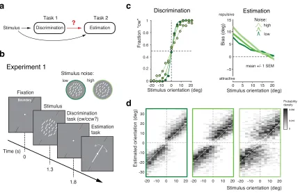
Figure 2.1: Post-decision biases in a perceptual task sequence. (a) Perceptual

decision-making in an estimation-discrimination task sequence: Does a discrimination judgment

causally affect a subject’s subsequent perceptual estimate? (b) Experiment 1: After being

presented with an orientation stimulus (array of lines), subjects first decided whether the overall array orientation was clockwise (cw) or counter-clockwise (ccw) of a discrimination boundary, and then had to estimate the actual orientation by adjusting a reference line with a joystick. Different stimulus noise levels were established by changing the orientation

variance in the array stimulus. (c) Psychometric functions and estimation biases (combined

subject). Estimation biases are only shown for correct trials and are combined across cw and ccw directions. Subjects show larger repulsive biases the noisier the stimulus and the

closer the stimulus orientation was to the boundary. (d) Distributions of estimates for the

(30)

2.3. Self-consistent Bayesian observer model

How are these post-decision biases explained? A Bayesian observer that regards the task

sequence as a two independent inference processes does not predict the biases. The observer

uses Bayesian statistics to determine the correct categorical judgment (e.g. ’cw’) based on

the stimulus response of a population of sensory neurons, and does the same to infer the

best possible estimate of the stimulus orientation (Fig. 2.2a). Consequently, this observer’s

discrimination judgment does not affect the estimation process; orientation estimates are

unimodally distributed around the true stimulus orientation and do not exhibit the

charac-teristic bimodal pattern that we have observed in Experiment 1 (Fig. 2.1d). In the context

of this paper, we refer to this model as the “independent” observer.

In contrast, we propose an observer model that regards the two tasks as causally

de-pendent (Fig. 2.2b); that is, by making the discrimination judgment the observer constrains

its subsequent estimation process to consider only those stimulus orientations that are

con-sistent with the judgment. It is as if the observer regards its own, subjective discrimination

judgment as an objective fact. Such behavior seems irrational (obviously, the judgment

could be incorrect) and furthermore leads to characteristic estimation biases away from the

discrimination boundary. It has the advantage, however, that the observer’s perceptual

in-ference process remains self-consistent throughout the entire task sequence at any moment

in time. We refer to this model as the “self-consistent” observer. It can be formulated

as a conditioned Bayesian model (Stocker and Simoncelli, 2007) that jointly accounts for

subjects’ behavior in both the discrimination and the estimation task. However, a closer

comparison between the predicted (Fig. 2.2b) and the measured distribution of the estimates

(Fig. 2.1d) reveals that this basic formulation does not capture all details accurately.

We formulated the self-consistent observer model as a two-step inference process over

the extended hierarchical generative model shown in Fig. 2.3a: Based on a noisy sensory

signalm, the observer first infers the category C (’cw’ or ’ccw’) by performing the

discrim-ination task and then infers the stimulus orientationθ in the estimation task. Because the

(31)

Model predictions Model predictions

Independent Bayesian observer a

Noise level

0 10 20 -10 -20 1 0 Fraction “cw” Discrimination judgement “cw”

Self-consistent Bayesian observer b

Noise level

0 10 20 -10

-20

Likelihoods low noise high noise ccw cw ccw cw Stimulus Sensory neurons 0 Orientation Bayesian Inference Conditional prior

Stimulus orientation (deg) Stimulus orientation (deg)

1 Fraction “cw” Bayesian Inference 0 20 -20 0 20

-20 -20 0 20

0 20

-20

Stimulus orientation (deg)

0 20

-20 -20 0 20

Stimulus orientation (deg) Orientation estimate

“cw” Bayesian

Inference BayesianInference Stimulus

Sensory neurons

0 Orientation

Discrimination

judgment Orientationestimate

Likelihoods low noise high noise Probability density 0.030 0.010 0

Discrimination Estimation Discrimination Estimation

cw Posteriors 0 Estimates Orientation Posteriors 0 Estimates Post-decision biases Orientation

Figure 2.2: Bayesian observer models for the perceptual task sequence. (a) The

discrim-ination judgment does not affect the estimated stimulus orientation for an observer who

considers both tasks independently. (b) In contrast, the self-consistent observer imposes a

causal dependency such that the judgment in the discrimination task (e.g. ’cw’) conditions

(32)

assume that estimation ofθmust rely on a noisy memory recallmm of the sensory signalm.

Inference onθis then conditioned on the preceding discrimination judgment (e.g. C = ’cw’),

which ultimately results in the characteristic repulsive estimation biases. Finally, we also

took into account that subjects’ report of their perceived stimulus orientation is corrupted

by motor noise. We measured motor noise for every subject in a control experiment (see

Figure supplement 2.12) and subsequently used these measured values for all model fits

and comparisons. The self-consistent observer model provides a full account of both the

observer’s discrimination judgment and orientation estimate in each trial and is thus jointly

predicting a subject’s psychometric function as well as the distribution of their orientation

estimates.

Figure 2.3b shows the model fit to the data from Experiment 1 for the combined

sub-ject. The stimulus noise level determines both the slope of the psychometric curves in the

discrimination task and the magnitude of the bias in the estimation task, which is well

predicted by the model. A comparison between the distributions of subjects’ estimates and

model estimates fully reveals the extent to which the model accurately accounts for the

observed human behavior (Fig. 2.3c; See Figure supplement 2.13 for a histogram

represen-tation). Note that all model predictions in this paper are the result of a joint fit to both the

measured psychometric functions of the discrimination task and the estimation distribution.

The self-consistent observer model can also account for the substantial individual

dif-ferences in behavior across subjects. While individual bias patterns are all repulsive, they

vary across subjects both in shape and magnitude (Fig. 2.4a). These variations are well

captured by the model and reflected in individual differences in the fit parameter values

such as the prior width and the level of sensory noise (Fig. 2.4b; see Figure supplement 2.14

for a goodness-of-fit analysis). Interestingly, all subjects seemed to substantially

overes-timate the width of the stimulus prior compared to the true stimulus distribution. This

did not come entirely as a surprise because subjects were never explicitly informed about

the stimulus range and thus had to learn it over the course of the experiment. Consistent

(33)

Fraction “cw” Noise: Model fit Data Bias (deg) −10 −5 0 5 10 15

0 5 10 15 20

b

c

a

0 0.2 0.4 0.6 0.8 1

0 10 20 -10

-20 -10 0

20 10

-20 -20 -10 0 10 20-20 -10 0 10 20

0 -10 10 20

-20 -20 -10 0 10 20-20 -10 0 10 20

0.030 0.010 0 -30 -20 -10 0 10 20 30 -30 -20 -10 0 10 20 30 Sensory measurement Stimulus orientation Category Working memory recall conditioned on judgment Model Data Experiment 1 Probability density

+ Motor noise

Discrimination Estimation

Figure 2.3: The self-consistent Bayesian observer model. (a) Directed graph representing

the generative hierarchical model: Sensory measurement m is a noisy sample of stimulus

orientationθ. Everyθbelongs to one of two categoriesC ={’cw’,’ccw’}. Given an observed

m, the self-consistent model first performs inference overC (discrimination task), and then

infers the value of θ conditioned on the preceding discrimination judgment (e.g. Cˆ =’cw’)

(estimation task). Inference for the estimation task is assumed to be based on a noisy

memory recall mm of the sensory measurementm. Conditioning on the categorical choice

sets the posterior p(θ|mm,Cˆ) to zero for all values ofθ that do not agree with the choice.

This shifts the posterior probability mass away from the discrimination boundary and results in the repulsive post-decision biases for any loss function that more strongly penalizes large errors than small ones. Because subjects were instructed to provide estimates as accurate

as possible we assumed a loss function that minimizes mean squared error (L2 loss). (b) We

jointly fit the observer model to all discrimination-estimation data pairs of the combined

data across all subjects in Experiment 1 (combined subject). (c) The model not only

predicts the mean estimation bias (as shown in (b)) but also the entire distributions of

estimates, including those trials where discrimination judgments were incorrect. Data and

model show the characteristic bimodal pattern for orientation estimates. Each column

(34)

-5 0 5 10 15 10

0 5 15 20 0 5 10 15 20 0 5 10 15 20 0 5 10 15 20 0 5 10 15 20

Bias (deg) -5 0 5 10 15 Bias (deg) 10

0 5 15 20 0 5 10 15 20 0 5 10 15 20 0 5 10 15 20 0 5 10 15 20

Noise

mean +/- 1 SEM

Noise (fit)

a b

S1 S2 S3 S4 S5

Experiment 1 Data

Model

Noise level SD (deg)

Prior width (deg)

0 10 20 30 40

S1 S2 S3 S4 S5 Sc

Subjects Memory Sensory 0 4 8 12 16

Figure 2.4: Experiment 1: Data and model fits for individual subjects.(a) Individual subjects

(S1 non-na¨ıve) showed substantial variations in their bias patterns (green curves). These variations are well explained by individual differences in the fit parameter values of the self-consistent model (blue curves). For example, the width of the prior directly determines the

location where the bias curves intersect with the x-axis. (b) Fit prior widths wp and noise

levels for the five individual subjects plus the combined subject (Sc). Subjects’ prior widths

suggest that they consistently overestimated the actual stimulus range in the experiment (±

21 degrees; arrow). For all subjects, fit sensory noiseσs was comparable and monotonically

dependent on the actual stimulus noise. Memory noiseσmwas mostly small as expected, yet

(35)

prior distribution was the only non-na¨ıve subject S1 who had plenty of extra exposure to

the stimulus range through the participation in various pilot experiments. Extracted noise

levels differ across subjects with the worst subject being approximately twice as noisy as the

best (non-na¨ıve subject S1), yet consistently increase for increasing stimulus noise levels.

2.4. Validating self-consistent Bayesian observer model

2.4.1. Key features of the model

We ran two additional experiments that were designed to specifically probe two key features

of the self-consistent model: Experiment 2 was aimed at testing how subject’s orientation

estimates were dependent on their precise knowledge of the stimulus prior and thus were

consistent with the results of Bayesian inference; Experiment 3 examined whether subjects

indeed treated their discrimination judgments as if they were correct. We recruited a new

set of subjects (S6-S9, plus S1) that performed both experiments. By jointly fitting the

data from both experiment, we also tested how well the model can generalize across tasks2.

Experiment 2 was identical to Experiment 1 except that at the beginning of each trial,

subjects were explicitly reminded of the total range within which the stimulus orientation

would occur in the trial (Fig. 2.5a). Our assumption was that an explicit display of the

stimulus range provided subjects with a better and presumably narrower representation

of the stimulus distribution (given that subjects seemed to substantially overestimate the

prior in Experiment 1). If so, then the self-consistent observer model would predict a

shift of the bias curves’ crossover point towards the discrimination boundary. As shown

in Figs. 2.5b, the measured bias curves indeed show the predicted shift compared to the

bias curves measured in Experiment 1 (Fig. 2.3b). This shift is also clearly visible in the

distributions of the orientation estimates (see Figure supplement 2.15 for distributions of

individual subjects), which is again accurately accounted for by the model (Fig. 2.5c).

In Experiment 3, we separated the discrimination judgment from the discrimination

task. Subjects were no longer asked to perform the orientation discrimination task but

2

(36)

b

c

a

_{Experiment 2}

0 5 10 15 20

Stimulus orientation (deg) Stimulus orientation (deg) Estimation task Discrimination task (cw/ccw?) Prior cue Model Model Time (s) 0 0.8 1.3 1.8 420 Data Data

0 5 10 15 20 mean +/- 1 SEM

−10 −5 0 5 10

15 Noise Noise (fit)

−10 −5 0 5 10 15 Bias (deg) 0 -10

20 10

-20 -20 -10 0 10 20 -20 -10 0 10 20

0 -10 10 20

-20 -20 -10 0 10 20 -20 -10 0 10 20 0.030 0.010 0 -30 -20 -10 0 10 20 30

-30 -20 -10 0 10 20 30 Probability density

Figure 2.5: Effect of the stimulus prior. (a) Experiment 2 was identical to Experiment 1

except that at the beginning of each trial, subjects were shown the total range within which

the stimulus orientation would occur in the trial (gray arc, subtending ± 21 degrees). (b)

We hypothesize that reminding subjects of the exact stimulus range at the beginning of each trial helps them to form a more accurate (and more narrow) representation of their stimulus prior. If subjects’ orientation estimates were indeed the result of the conditioned Bayesian inference as assumed by the self-consistent observer model, then the bias curves should shift towards the discrimination boundary. The data support this prediction: Subjects’ bias curves (combined subject, see Fig. 2.7 for individual subjects) are shifted towards the

discrimination boundary compared to Exp. 1. (c) As with Exp.1, the fit self-consistent

(37)

Given correct answer (”cw”)

a

b

c

−10 −5 0 5 10 15

0 5 10 15 20 0 5 10 15 20

Experiment 3

Color discrimination task (red/green?) Time (s) 0 0.5 0.8 1.3 1.8 Noise Estimation task Model Data Noise (fit) −10 −5 0 5 10 15 Bias (deg) 0

-10 10 20

-20 -20 -10 0 10 20-20 -10 0 10 20

0

-10 10 20

-20 -20 -10 0 10 20-20 -10 0 10 20

Model

Data

0.030 0.010 0 -30 -20 -10 0 10 20 30

-30 -20 -10 0 10 20 30 Probability density

Figure 2.6: Self-made vs. given category assignment.(a) Experiment 3: Instead of

perform-ing the discrimination judgment themselves, subjects were provided with a cue indicatperform-ing the correct category assignment right before the stimulus was presented. Then, after stimu-lus presentation, subjects first performed an unrelated color discrimination task in place of the orientation discrimination task (they needed to remember the randomly assigned color (red/green) of the cue indicating the correct category) before indicating their perceived

stimulus orientation. (b) According to our model we should see similar estimation biases

in Exp. 2 and 3, which is indeed what we found: because the data are from the same

subjects we can directly compare the bias curves with the results from Exp. 2. (c) Again,

the fit model well accounts for the overall distribution of orientation estimates (combined subject; see Figure supplement 2.16 for distributions for individual subjects)). Because the discrimination judgment was given and always correct independent of the noise in the

sensory measurementm, estimates only occurred in the “correct” quadrants. For the same

(38)

instead were signaled right at the beginning of each trial whether the stimulus orientation

would be cw or ccw (Fig. 2.6a). Subjects were instructed that this categorical information

was always correct, which it was. They then performed an unrelated color discrimination

task before finally performing the estimation task. The self-consistent model predicts

es-timation biases that are basically identical to those of Experiment 2 because it assumes

that subjects treat their own judgment as correct when performing the estimation task.

Indeed, as shown in Fig. 2.6b, subjects’ estimation biases are very similar to the biases in

Experiment 2 (Fig. 2.5b). Because both Experiment 2 and 3 were conducted on the same

set of subjects, the results are directly comparable. We can rule out that subjects may

have ignored the given category assignment in Experiment 3 and implicitly performed the

orientation discrimination task instead. If this were the case, then subjects would have

ex-hibited a large fraction of inconsistent trials (i.e. trials in which the estimated orientation

was not in agreement with the given correct answer) in particular for orientations close to

the discrimination boundary. This was not the case as we observed only small fractions

of inconsistent trials (4% on average) that were of similar magnitude as the error rates for

the (irrelevant) color discrimination task (2%). We discuss these inconsistent trials in more

detail in the next section below.

We again extended our analysis to individual subjects’ behavior. Figure 2.7a shows

subjects’ estimation biases in both experiments as well as the corresponding model

predic-tions based on a joint fit to data from both Experiment 2 and 3. Bias patterns, while quite

variable across subjects, are consistent across the two experiments for each subject. This

confirms that the impact of the categorical discrimination judgment on the perceived

orien-tation does not depend on whether the judgment was performed by the subjects themselves

or not. The model captures both the inter-subject as well as the within-subject variability

across the two experiments. Biases are slightly smaller in Experiment 3 compared to

Exper-iment 2 for stimulus orientations close to the boundary. As shown in Fig. 2.7b, the model

correctly predicts this difference because the self-made discrimination judgments in

(39)

S1 S6 S7 S8 S9

a _b

c mean +/- 1 SEM

Experiment 2 Experiment 3 -5 0 5 10 15 10

0 5 15 20 0 5 10 15 20 0 5 10 15 20 0 5 10 15 20 0 5 10 15 20

10

0 5 15 20 0 5 10 15 20 0 5 10 15 20 0 5 10 15 20 0 5 10 15 20

10

0 5 15 20 0 5 10 15 20 0 5 10 15 20 0 5 10 15 20 0 5 10 15 20

10

0 5 15 20 0 5 10 15 20 0 5 10 15 20 0 5 10 15 20 0 5 10 15 20

Bias (deg) -5 0 5 10 15 Bias (deg) -5 0 5 10 15 Bias (deg) -5 0 5 10 15 Bias (deg)

Prior width (deg)

0 10 20 30

S1 S6 S7 S8 S9 Sc

Subjects

Data

Model

Noise level SD (deg)

Mean Bias Exp 3 (deg)

Mean Bias Exp 2 (deg)

Memory Sensory

S1 S6 S7 S8 S9 Sc

Noise Noise (fit) 2 4 6 8 10 12 2 4 6 8 10 12

2 4 6 8 10 12

0 4 8 12 16

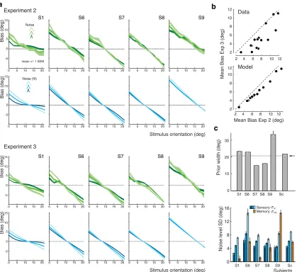
Figure 2.7: Experiments 2 and 3: Joint fit to data for individual subjects.(a) Five subjects

(S1, S6-9) participated both in Exp. 2 and 3. We performed a joint model fit to the data from both experiments for every subject. Each column shows data (green curves) and model fit (blue curves) for a particular subject. As in Exp. 1, the bias pattern across subjects

shows substantial variability yet is strikingly similar between the two experiments. (b)

Comparing the mean biases observed in Exps. 2 and 3 reveals that biases in Exp. 3 are slightly smaller for stimulus orientations close to the boundary. This effect is predicted by

the model. (c) Prior widthswp and noise levels from the joint fit for individual subjects and

Self-Consistency In Sequential Decision-Making

University of Pennsylvania

ScholarlyCommons

Publicly Accessible Penn Dissertations

2018

Self-Consistency In Sequential Decision-Making

Long Luu

Follow this and additional works at:

https://repository.upenn.edu/edissertations

Part of the

Neuroscience and Neurobiology Commons, and the

Psychology Commons

Recommended Citation

Self-Consistency In Sequential Decision-Making

Acknowledgment

ABSTRACT

TABLE OF CONTENTS

List of figures

Chapter 1

Introduction

1.1. Sequential dependency in cognitive judgments

1.2. Sequential dependency in perceptual judgments

1.3. Bayesian decision theory

1.4. Supplemental-psychophysics methods

b

a

c

v

v

m

d

m

t

m

Chapter 2

Self-consistent inference

2.1. Introduction

2.2. Replicating choice-induced bias

a

c

b

d

2.3. Self-consistent Bayesian observer model

b

c

a

2.4. Validating self-consistent Bayesian observer model

b

c

a

a

b

c