Limitations of Correlation-Based Inference in Complex
Virus-Microbe Communities
Ashley R. Coenen,
bJoshua S. Weitz
a,baSchool of Biological Sciences, Georgia Institute of Technology, Atlanta, Georgia, USA
bSchool of Physics, Georgia Institute of Technology, Atlanta, Georgia, USA
ABSTRACT
Microbes are present in high abundances in the environment and in
human-associated microbiomes, often exceeding 1 million per ml. Viruses of
mi-crobes are present in even higher abundances and are important in shaping
micro-bial populations, communities, and ecosystems. Given the relative specificity of viral
infection, it is essential to identify the functional linkages between viruses and their
microbial hosts, particularly given dynamic changes in virus and host abundances.
Multiple approaches have been proposed to infer infection networks from time
series of
in situ
communities, among which correlation-based approaches have
emerged as the
de facto
standard. In this work, we evaluate the accuracy of
correlation-based inference methods using an
in silico
approach. In doing so, we
compare predicted networks to actual networks to assess the self-consistency of
correlation-based inference. At odds with assumptions underlying its widespread
use, we find that correlation is a poor predictor of interactions in the context of viral
infection and lysis of microbial hosts. The failure to predict interactions holds for
methods that leverage product-moment, time-lagged, and relative-abundance-based
correlations. In closing, we discuss alternative inference methods, particularly
model-based methods, as a means to infer interactions in complex microbial communities
with viruses.
IMPORTANCE
Inferring interactions from population time series is an active and
on-going area of research. It is relevant across many biological systems—particularly in
virus-microbe communities, but also in gene regulatory networks, neural networks,
and ecological communities broadly. Correlation-based inference— using correlations
to predict interactions—is widespread. However, it is well-known that “correlation
does not imply causation.” Despite this, many studies apply correlation-based
infer-ence methods to experimental time series without first assessing the potential scope
for accurate inference. Here, we find that several correlation-based inference
meth-ods fail to recover interactions within
in silico
virus-microbe communities, raising
questions on their relevance when applied
in situ
.
KEYWORDS
correlation, inference, interaction network, microbial ecology, viral
ecology
V
iruses of microbes are ubiquitous and highly diverse in marine, soil, and
human-associated environments. Viruses interact with their microbial hosts in many ways.
For example, they can transfer genes between microbial hosts (1, 2), alter host
physi-ology and metabolism (3, 4), and redirect the flow of organic matter in food webs
through cell lysis (5, 6). Viruses are important parts of microbial communities, and
characterizing the interactions between viruses and their microbial hosts is critical for
understanding microbial community structure and ecosystem function (5, 7–9).
A key step in characterizing virus-microbe interactions is determining which viruses
can infect which microbes. Viruses are known to be relatively specific but not exclusive
Received8 June 2018Accepted24 July 2018 Published28 August 2018 CitationCoenen AR, Weitz JS. 2018. Limitations of correlation-based inference in complex virus-microbe communities. mSystems 3:e00084-18.https://doi.org/10 .1128/mSystems.00084-18.
EditorSeth Bordenstein, Vanderbilt University Copyright© 2018 Coenen and Weitz. This is an open-access article distributed under the terms of theCreative Commons Attribution 4.0 International license.
Address correspondence to Joshua S. Weitz, [email protected].
Ecological and Evolutionary Science
crossm
on September 8, 2020 by guest
http://msystems.asm.org/
in their microbial host range. Individual viruses may infect multiple strains of an isolated
microbe, or they may infect across genera as part of complex virus-microbe interaction
networks (10, 11). For example, cyanophage can infect both
Prochlorococcus
and
Synechococcus
, which are two distinct genera of marine cyanobacteria (12). However,
knowledge of viral host range remains limited, because existing experimental methods
for directly testing for viral infection are generally not applicable to an entire
in situ
community. Culture-based methods such as plaque assays are useful for checking for
viral infection at the strain level and permit high confidence in their results, but they are
not broadly applicable, as many viruses and microbes are difficult or currently
impos-sible to isolate and culture (1). Partially culture-independent methods, such as viral
tagging (13, 14) and digital PCR (15), overcome some of these hurdles but only for
particular targetable viruses and microbes. Similarly, single-cell genome analysis is able
to link individual viruses to microbial hosts (16–18) but for a relatively small number of
cells.
Viral metagenomics offers an alternate route for probing virus-microbe interactions
for entire
in situ
communities, bypassing culturing altogether (19–21). The viral
se-quences obtained from metagenomes can be analyzed directly using
bioinformatics-based methods to predict microbial hosts (22, 23), although such methods may be
appropriate only for a subset of viruses (phages and archaeal viruses but not eukaryotic
viruses) and putative hosts (prokaryotes but not eukaryotes). Alternatively,
meta-genomic sampling of a community over time can provide estimates of the changing
abundances of viral and microbial populations at high resolution in time and across
taxonomic groups. Once these high-resolution time series are obtained, they can be
used to predict virus-microbe interactions using a variety of statistical and
mathemat-ical inference methods (for reviews, see references 24 to 28).
Correlation and correlation-based methods are among the most widely used
net-work inference methods for microbial communities (25). For example, extended local
similarity analysis (eLSA) is a correlation-based method that allows for both local and
time-lagged correlations (29–31), and it has been used to infer interaction networks in
communities of marine bacteria (32, 33), bacteria and phytoplankton (34, 35), bacteria
and viruses (36), and bacteria, viruses, and protists (37, 38). In addition, several
correlation-based methods have been developed to address challenges associated with
the compositional nature of “-omics” data sets (25, 39), including sparse correlations for
compositional data (SparCC) (40).
Regardless of the particular details of these methods, all correlation-based inference
operates on the same core assumptions that interacting populations trend together
(are correlated) and that noninteracting populations do not trend together (are not
correlated). Particular correlation-based methods may relax or augment this
assump-tion. For example, with eLSA, the trends may be time lagged (29–31); with simple rank
correlations, the trends may be nonparametric; and with compositional methods like
SparCC, the trends may occur between ratios of relative abundances (40). In
commu-nities with only a few populations and simple interactions, population trends may
indeed be indicative of ecological mechanism. In these contexts, some
correlation-based methods have been shown to recapitulate microbe-microbe interactions with
limited success (25). Typically, however, the challenge of inferring interaction networks
applies to diverse communities and complex ecological interactions. Microbial
com-munities often have dozens, hundreds, or more distinct populations, each of which may
interact with many other populations through nonlinear mechanisms such as viral lysis,
as well as be influenced by fluctuating abiotic drivers. In these contexts, the relationship
between correlation and ecological mechanism is poorly understood. Often,
correla-tions do not have a simple mechanistic interpretation, a well-known adage (“correlation
does not imply causation”) that is often disregarded.
Despite the challenge of interpretation, correlation-based inference methods are
widely used with
in situ
data sets (25, 29–40). Benchmarking inferred networks—
connecting correlations to specific ecological mechanisms—is difficult. In the context of
lytic infections of environmental microbes by viruses, there is (usually) no existing “gold
Coenen and Weitz
on September 8, 2020 by guest
http://msystems.asm.org/
standard” interaction network with which to validate inferred interactions. Therefore, in
this work, we take an
in silico
approach to assess the accuracy of correlation-based
inference. To do this, we simulate virus-microbe community dynamics with an
inter-action network which is prescribed
a priori
and use it to benchmark inferred networks.
Several existing studies have applied similar
in silico
approaches in the case of both
microbe-microbe and microbe-virus interactions and found that simple Pearson
corre-lation (39, 41) and several correcorre-lation-based methods (25) either fail or are inconsistent
in recapitulating interaction networks. Here, we provide an in-depth assessment of the
potential for correlation-based inference in diverse communities of microbes and
viruses. As we show, correlation-based inference fails to recapitulate virus-microbe
interactions and performs worse in more diverse communities. The failure of
correlation-based inference in this context raises concerns over its use in inferring
microbe-parasite interactions as well as microbe-predator and microbe-microbe
inter-actions more broadly.
RESULTS
Standard Pearson correlation.
We calculated the standard Pearson correlation
networks for an ensemble of
in silico
communities that varied in network size and
network structure. For each network size
N
⫽
10, 25, 50, we generated 20 unique
interaction networks. Ten of the networks were generated so that they were distributed
along a range of nestedness values, and the other ten were generated so that they were
distributed along a range of modularity values (see “Generating interaction networks
and characterizing network structure” in Materials and Methods). For each interaction
network, a single set of life history traits were generated to ensure coexistence using
biologically feasible ranges (see “Choosing life history traits for coexistence” in Materials
and Methods). The mechanistic model for the community dynamics is described below
in “Dynamic model of a virus-microbe community.” Time series were simulated
accord-ing to “Simulataccord-ing and samplaccord-ing time series” with
␦
⫽
0.3, that is, the initial conditions
were the fixed-point values perturbed by 30% (for additional values of
␦
, see Fig. S4 in
the supplemental material). For
␦
⫽
0.3, the mean coefficient of variation was 12% for
host time series and 4% for virus time series (Fig. S1). The time series were sampled
during the transient dynamics to represent
in situ
communities which are likely
perturbed from equilibrium due to changing environmental conditions and intrinsic
feedback. We sampled the time series every 2 h for 200 h, that is, we took 100 samples
(for additional sample frequencies, see Fig. S7).
For each
in silico
community, we calculated the standard Pearson correlation
network as described in “Standard and time-delayed Pearson correlation networks” in
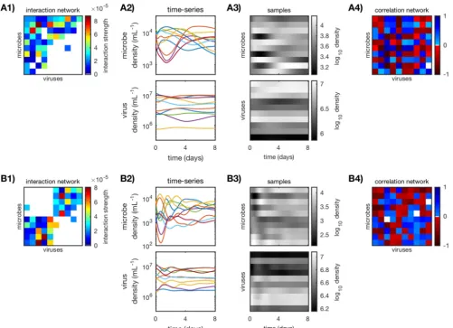
Materials and Methods. Two examples of
in silico
communities of size
N
⫽
10 are shown
in Fig. 1 with their simulated time series, log-transformed samples, and resulting
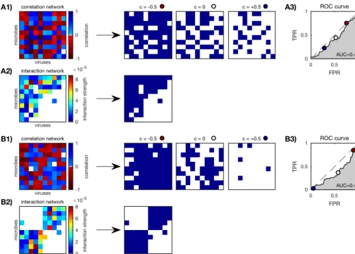
correlation networks. The correlation networks were scored against the original
inter-action networks by computing area under the curve (AUC) as described in “Scoring
correlation network accuracy”. The procedure for computing AUC is shown in Fig. 2 for
the two examples of
in silico
communities.
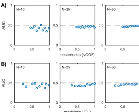
AUC values for all
in silico
communities are shown in Fig. 3. Across different network
sizes and network structures, the AUC is approximately 1/2, implying that standard
Pearson correlation networks lack predictive power. Similar results were found when
changing the initial condition perturbation
␦
(Fig. S4) and the sampling frequency
(Fig. S7). There are some instances where the AUC does deviate from 1/2 for the smaller
networks (
N
⫽
10), although these deviations are small (
⬇⫾
10%). Interestingly, these
deviations tend to be negative, indicating a misclassification of the interaction
condi-tion, that is, negative correlations are slightly better predictors of interaction than
positive correlations. Overall, however, the deviations disappear for larger networks
(
N
⫽
50), implying that they are exceptions rather than the norm. We completed
identical analyses for additional correlation metrics, in particular Spearman correlation
and Kendall correlation (see Fig. S2). We found similar results, reinforcing our
on September 8, 2020 by guest
http://msystems.asm.org/
sion that simple correlations between time series are poor predictors of the underlying
interaction network.
Time-delayed Pearson correlation.
Given the results of the previous section
(“Standard Pearson correlation”)—that standard correlations do not recapitulate
inter-actions—we computed time-delayed correlation networks for the same ensemble of
in
silico
communities. The addition of time delays to standard correlation approaches is
motivated by a large body of theoretical work on predator-prey dynamics, where both
predator and prey populations oscillate but with a phase delay between them (42).
Similar results hold for the phase delay in simple phage-bacteria dynamics (43).
Time-delayed correlations are the basis of several existing correlation-based inference
methods, including eLSA (29–31).
For this analysis, we used the same ensemble of
in silico
communities (networks with
network sizes
N
⫽
10, 25, 50 and different levels of nestedness and modularity),
simulated time series (
␦
⫽
0.3; see Fig. S5 in the supplemental material), and sample
frequency (2 h; Fig. S8) as before (see “Standard Pearson correlation” above for time
series). We calculated the time-delayed Pearson correlation networks as described in
“Standard and time-delayed Pearson correlation networks” below, where for each
virus-host pair, virus
j
is sampled later in time relative to host
i
by the time delay value
ij(for Spearman correlation and Kendall correlation, see Fig. S3). Each delay is chosen
FIG 1 Calculating standard Pearson correlation networks for anin siliconested (A) and a modular (B) community (N⫽10). (A1 and B1) Original weighted interaction networks, generated as described in “Generating interaction networks and characterizing network structure” and “Choosing life history traits for coexistence” in Materials and Methods. (A2 and B2) Simulated time series of the virus-microbe dynamic system as described in “Simulating and sampling time series” (␦⫽0.3). (A3 and B3) Log-transformed samples, sampled every 2 h for 200 h from the simulated time series. (A4 and B4) Pearson correlation networks, calculated from log-transformed samples as described in “Standard and time-delayed Pearson correlation networks.”
Coenen and Weitz
on September 8, 2020 by guest
http://msystems.asm.org/
such that the absolute value of the correlation for the virus-host pair is maximized.
Since the optimal time delay is not known in advance, delays between 0 h and half the
sample length
ts
(
ts
/2
⫽
100 h) were considered. The number of samples used to
compute each correlation coefficient was kept fixed at
S
⫽
100 (sample duration,
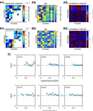
200 h). Time-delayed Pearson correlation networks for the two example
in silico
communities of size
N
⫽
10 are shown in Fig. 4A and B. AUC was computed as
described in “Scoring correlation network accuracy” below.
AUC values for all
in silico
communities are shown in Fig. 4C. For the small networks
(
N
⫽
10), there are a few particular networks that have AUC scores greater than 1/2. For
the remaining small networks and the large networks (
N
⫽
25, 50), AUC is
⬇
1/2,
implying that time-delayed Pearson correlation lacks predictive power for these
net-works. Similar results were found for alternate correlation metrics (Spearman and
Kendall correlations; Fig. S3), initial condition perturbations
␦
(Fig. S5), and sampling
frequencies (Fig. S8). Because AUC deviates from 1/2 for only a few small networks and
this deviation disappears for large networks, it should be considered an exception
rather than the norm for time-delayed Pearson correlation.
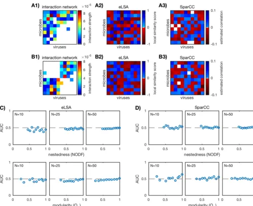
Correlation-based methods eLSA and SparCC.
We performed a similar
in silico
analysis using eLSA (29–31) and SparCC (40), two established correlation-based
infer-ence methods that are widely used with
in situ
time series data. We used the same
FIG 2 Scoring correlation network accuracy of anin siliconested (A) and a modular (B) community (N⫽10; see Fig. 1) as described in “Scoring correlation network accuracy” in Materials and Methods. (A1 and B1) Correlation networks are binarized according to thresholdscbetween⫺1 and⫹1, three of which are shown here (c⫽ ⫺0.5, 0, and 0.5). (A2 and B2) Original interaction networks are also binarized. (A3 and B3) True-positive rate (TPR) versus false-positive rate (FPR) of the binarized correlation networks for each thresholdc. Three example thresholds (c⫽ ⫺0.5, 0, and 0.5) are marked (red, white, and dark blue circles). The “nondiscrimination” line (gray dashed line) is where TPR⫽FPR. The AUC or area under the ROC is a measure of relative TPR to FPR over all thresholds; AUC⫽1 is a perfect result.
on September 8, 2020 by guest
http://msystems.asm.org/
ensemble of
in silico
communities as before (network sizes
N
⫽
10, 25, 50 and networks
with different levels of nestedness and modularity), along with the simulated time
series (
␦
⫽
0.3; see Fig. S6), sample frequency (2 h; see Fig. S9) and sample duration
(200 h). We implemented eLSA and SparCC as described in “eLSA networks” and
“SparCC networks,” respectively, in Materials and Methods. eLSA and SparCC predicted
networks for the two examples of
in silico
communities of size
N
⫽
10 are shown in
Fig. 5A and B. AUC was computed as before and as described in “Scoring correlation
network accuracy” below.
AUC values for all
in silico
communities are shown in Fig. 5C. We see the same trends
as with standard correlation and time-delayed correlation (see Fig. 3 and 4). Similar
results hold for different values of the initial condition perturbation
␦
(Fig. S6) and
sampling frequency (Fig. S9). For small networks (
N
⫽
10), there are a few AUC scores
that deviate weakly from 1/2 (
⬇⫾
10%). Interestingly, AUC scores for eLSA tend to be
negative, implying a misclassification of interaction. AUC converges to 1/2 as network
size increases (
N
⫽
25, 50), indicating that the AUC scores for small networks may
themselves be spurious.
DISCUSSION
Using
in silico
virus-microbe community dynamics, we calculated correlation
net-works among viral and microbial population time series samples. We tested the
accuracy of several different types of correlation and time-delayed correlation (Pearson,
Spearman, and Kendall correlation) and existing correlation-based inference methods
(eLSA and SparCC). The correlation networks for all of these implementations failed to
effectively predict the original interaction networks, as quantified by the AUC score.
Failure persisted across variation in network structure, network size, degree of initial
condition perturbation (i.e., scaling the variability of dynamics), and sampling
fre-quency. We therefore conclude that these correlation-based inference methods do not
meaningfully predict interactions given this mechanistic model of virus-microbe
com-munity dynamics.
Earlier, we stated the core assumption of correlation-based inference—that
inter-acting populations are correlated and that noninterinter-acting populations are not
corre-lated. While this core assumption may sometimes hold in small microbe-only
commu-nities with simple interaction mechanisms (25), we find that it does not necessarily hold
FIG 3 AUC values for standard Pearson correlation for the ensemble of nested (A) and modular (B) communities over three network sizesN⫽10, 25, 50 (20 communities for each network size). AUC is computed as described in “Scoring correlation network accuracy” in Materials and Methods. Each plotted point corresponds to a uniquein silicocommunity. The dashed lines mark AUC⫽1/2 and imply that the predicted network did no better than random guessing.Coenen and Weitz
on September 8, 2020 by guest
http://msystems.asm.org/
in more-complex virus-microbe communities. Each inference method also faces
chal-lenges unique to its formulation: eLSA in particular uses a nonstationary data
transfor-mation which may induce additional spurious correlations. We considered communities
with microbes and viruses that interacted through a nonlinear mechanism (infection
and lysis) across a spectrum of network sizes and network structures. We found that
correlation-based inference performed poorly given variation in these network
prop-erties but that there was greater variation in performance for small networks. Because
this variation is relatively small and disappears for larger networks, successful
predic-tions for small networks may themselves be spurious. Namely, for a small network (e.g.,
N
⬍
10), there is a greater probability of randomly guessing the interactions correctly
because the space of possible networks is smaller.
Our results raise concerns about the use of correlation-based methods on
in situ
FIG 4 Performance of time-delayed Pearson correlation. (A1 and B1) Two examples ofin silicointeraction networks (N⫽10). (A2 and B2) Time delaysijfor each virus-host pair, chosen so that the absolute value of the correlation is maximized. (A3 and B3) Time-delayed Pearson correlation networks calculated as described in “Standard and time-delayed Pearson correlation networks” in Materials and Methods. (C) AUC values for the ensemble of nested (top row) and modular (bottom row) communities over three network sizesN⫽10, 25, 50 (20 communities for each network size). Each plotted point corresponds to a unique in silicocommunity. The dashed lines mark AUC⫽1/2 and imply that the predicted network did no better than random guessing.on September 8, 2020 by guest
http://msystems.asm.org/
data sets, since a typical community under consideration will have dozens or more
interacting strains and therefore will not be in the low-diversity microbe-only regime
explored by Weiss et al. (25). Additional challenges such as external environmental
drivers, measurement noise, and system stochasticity must also be carefully considered
before applying correlation-based methods to
in situ
data sets. Although the degree of
variability of dynamics had no effect on inference quality here, it may also be an
important consideration for both experimental design and choice of inference method.
For example, the model-based inference method examined by Jover et al. (44) performs
better when dynamics are highly variable. On the other hand, cooccurrence-based
inference methods, which require samples across space instead of time, may enable
inference across different baseline environmental conditions even if the dynamics
within a given environment are relatively stable.
In light of the poor performance of correlation-based methods, we advocate for
increased studies of model-based inference. Model-based inference methods operate
by first assuming an underlying dynamic model for the community (such as the one
used in this article [see equations 1 and 2 below]). The dynamic model is then used to
FIG 5 Performance of correlation-based inference methods eLSA and SparCC. (A1 and B1) Two examples ofin silicointeraction networks (N⫽10). (A2 and B2) eLSA-predicted network computed as described in “eLSA networks” in Materials and Methods. (A3 and B3) SparCC-predicted network computed as described in “SparCC networks” (color bar adjusted for visibility). (C and D) AUC values for the ensemble of nested (top row) and modular (bottom row) communities over three network sizesN⫽10, 25, 50 (20 communities for each network size). Each plotted point corresponds to a uniquein silicocommunity. The dashed lines mark AUC⫽1/2 and imply that the predicted network did no better than random guessing.
Coenen and Weitz
on September 8, 2020 by guest
http://msystems.asm.org/
formulate an objective function for an optimization or regression problem, where the
solution is the interaction network which best describes the sampled community time
series (for example, see references 39, 41, 49, 50, 51, and 52). Unlike correlation-based
methods which assume that similar trends in population indicate interaction,
model-based inference has the potential to be tailored to complex communities and
environ-ments while leveraging existing knowledge about ecological mechanisms. Given
fa-vorable results of
in silico
benchmarking of model-based inference methods (39, 41,
44–47), it will be important to investigate the efficacy of model-based inference
methods for complex microbial and viral communities in practice.
MATERIALS AND METHODS
Dynamic model of a virus-microbe community.We model the ecological dynamics of a virus-microbe community with a system of nonlinear differential equations:
whereHiandVjrefer to the population density of microbial hostiand virusj, respectively. There areNH different microbial host populations andNVdifferent virus populations. For our purposes, a “population” is a group of microbes or viruses with identical life history traits, that is microbes or viruses that occupy the same functional niche.
In the absence of viruses, the microbial hosts undergo logistic growth with growth ratesri. The microbial hosts have a community-wide carrying capacityK, and they compete with each other for resources both inter- and intraspecifically with competition strengthaii=. Each microbial host can be infected and lysed by a subset of viruses determined by the interaction termMij. If microbial hostican be infected by virusj,Mij⫽1; otherwise,Mij⫽0. The collection of all the interaction terms is the interaction network represented by matrixMof sizeNHbyNV. The adsorption rateijdenotes how frequently microbial hostiis infected by virusj.
Each virusj=s population grows from infecting and lysing their hosts. The rate of virusj=s growth is determined by its host-specific adsorption rate ijand host-specific burst sizeij, which is the net number of new virions per infected host cell. The quantityM˜ij⫽Mijijijis the effective interaction
strength between virusjand hosti, and the collection of all the interaction strengths is the weighted interaction networkM˜.Finally, the viruses decay at ratesmj.
Generating interaction networks and characterizing network structure.Virus-microbe interac-tion networks, denotedM, are represented as bipartite networks or matrices of sizeNHbyNVwhereNH is the number of microbial host populations andNVis the number of virus populations. The elementMij is 1 if microbe populationiand virus populationjinteract and 0 if the two populations do not interact. In this paper, we consider only square networks (N⫽NH⫽NV), although the analysis is easily extended to rectangular networks. We consider three network sizesN⫽10, 25, 50.
For each network sizeN, we generate an ensemble of networks with different degrees of nestedness and modularity (Fig. 6). We first generate the maximally nested (Fig. 6A) and maximally modular (Fig. 6B) networks of sizeNusing the BiMat Matlab package (48). In order to achieve maximal nestedness and modularity, the network fillF(fraction of interacting pairs) is fixed atF⫽0.55 for the nested networks andF⫽0.5 for the modular networks. For the modular networks, the number of modules is set to 2, 5, and 10 for the three network sizes, respectively.
To generate networks that vary in nestedness and modularity, we perform the following “rewiring” procedure. Beginning with the maximally nested or maximally modular network, we randomly select an interacting virus-microbe pair (Mij⫽1) and a noninteracting virus-microbe pair (Mi=j=⫽0) and exchange their values. We do not allow exchanges that would result in an all-zero row or column, as that would isolate the microbe or virus population from the rest of the community. We continue the random selection of pairs without replacement until the desired nestedness or modularity has been achieved. To calculate nestedness and modularity, we use the default algorithms in the BiMat Matlab package. The nestedness metric used is NODF (nestedness metric based on overlap and decreasing fill) (49), and the algorithm used to calculate modularity is AdaptiveBRIM (50). The modularity is additionally normalized according to a maximum theoretical modularity as detailed in reference 51.
Choosing life history traits for coexistence.The life history traits for a given interaction network are chosen to ensure that all microbial host and virus populations can coexist, adapted from reference 52.
First, we sample target fixed-point densitiesHi
*
andVj
*
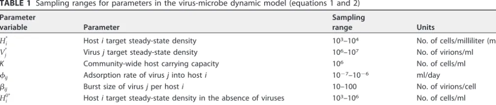
for each microbial host and virus population. In addition, we sample adsorption ratesijand burst sizesij. All of these parameters are independently and randomly sampled from uniform distributions with biologically feasible ranges specified in Table 1. We use a fixed carrying capacity densityK⫽106cells/ml for all parameter sets.
on September 8, 2020 by guest
http://msystems.asm.org/
Next, we sample microbe-microbe competition termsaii=. We introduce an additional constraint that microbial populations should coexist in the absence of all viruses. To this end, we sample target virus-free fixed-point densitiesHi
0*
from a uniform distribution with a range specified in Table 1. After sampling, the
Hi0*remains fixed. According to equation 1, coexistence in the virus-free setting is satisfied when
K⫽
冘
i'
NH
aii'Hi'
0*
(3)
for each microbial hosti. To start, we set all intraspecific competition to one (aii⫽1) and all interspecific competition to zero (aii=⫽0 fori=⫽i). Then, for each microbial hosti, we randomly choose an index k⫽iand sampleaikuniformly between zero and one. If the updated sum in equation 3 does not exceed the carrying capacityK, we repeat for a new indexk. Once the carrying capacity is exceeded, we adjust the most recentaikso that equation 3 is satisfied exactly.
Finally, the viral decay ratesmjand host growth ratesriare computed from the fixed-point versions of equations 1 and 2:
mj⫽
冘
i NHMijijijHi
*
(4)
ri⫽
冉
冘
j NVMijijVj
*
冊
⁄
冢
1⫺冘
i'NH
aii'Hi'
*
K
冣
(5)Simulating and sampling time series. We use Matlab’s nativeODE45function to numerically simulate the virus-microbe dynamic model specified above in “Dynamic model of a virus-microbe community” with interaction network and life history traits generated as described in “Generating interaction networks and characterizing network structure” and “Choosing life history traits for coexis-tence” above. We use a relative error tolerance of 10⫺8. Initial conditions are chosen by perturbing the
FIG 6 Examples of interaction networks characterized by nestedness (A) and modularity (B). The networks shown here have sizeN⫽10 and fillF⫽0.55 (A) andF⫽0.5 (B). Within each network, rows represent microbe populations and columns represent virus populations, while navy squares indicate interaction (Mij⫽1). Networks were generated as described in “Generating interaction networks and characterizing network structure” in Materials and Methods. Nestedness (NODF) and modularity (Qb) were measured with the BiMat package and are arranged in their most nested or most modular forms (48).
TABLE 1 Sampling ranges for parameters in the virus-microbe dynamic model (equations 1 and 2)
Parameter
variable Parameter
Sampling
range Units
Hi* Hostitarget steady-state density 103–104 No. of cells/milliliter (ml)
Vj* Virusjtarget steady-state density 106–107 No. of virions/ml
K Community-wide host carrying capacity 106 No. of cells/ml
ij Adsorption rate of virusjinto hosti 10⫺7–10⫺6 ml/day
ij Burst size of virusjper hosti 10–100 No. of virions/cell
Hi0* Hostitarget steady-state density in the absence of viruses 103–106 No. of cells/ml
aii' Competitive effect of hosti=on hosti 0–1
Coenen and Weitz
on September 8, 2020 by guest
http://msystems.asm.org/
fixed-point densitiesHi
*
andVj
*
by a multiplicative factor␦where the sign of␦is chosen randomly for each microbial host and virus population. We note that␦can be used to tune the amount of variability in the simulated time series (see Fig. S1 in the supplemental material).
After simulating virus and microbe time series, we sample the time series at regularly spaced sample times (every 2 h) for a fixed duration (200 h, or 100 samples). Therefore, for each virus and each microbe in the community, we takeSsamples at timest1,. . .,tS. We use the same sampling frequency and the same S for each inference method, except for time-delayed correlation (see “Standard and time-delayed Pearson correlation networks” below).
Standard and time-delayed Pearson correlation networks.We assumeSregularly spaced sample timest1,. . .,tSfor each host typeHiand each virus typeVj. The samples are log transformed, that is
hi共tk兲⫽log10Hi共tk兲andvj共tk兲⫽log10Vj共tk兲for each sampled time pointtk. The standard Pearson correlation coefficient between hostiand virusjis then
rij⫽ k
冘
⫽1 S关
hi共
tk兲
⫺hi兴
关
vj共
tk兲
⫺vj兴
冑
k冘
⫽S1关
hi共
tk兲
⫺hi兴
2
冑
冘
k⫽1
S
关
vj共
tk兲
⫺vj兴
2(6)
wherehi⫽
1
S
冘
kS⫽1hi共tk兲andvj⫽1
S
冘
k⫽1S
vj共tk兲are the sample means. The correlation coefficients for all
virus-host pairs are represented as a bipartite matrixRof sizeNH⫻NVanalogous to the interaction network (see “Generating interaction networks and characterizing network structure” above).
Time-delayed correlations are computed by sampling the virus time series later in time. Each virus-host pair may have a unique time delayij. For example, if hostiis sampled at timest1,. . .,tS, then virusjis sampled at timest1⫹ij,. . .,tS⫹ij. We keep the number of samplesSfixed, and consequently allow virusjto be sampled beyond the final sample timetSof the hosts. The time-delayed Pearson correlation coefficient is
rij⫽
冘
k⫽1S
关
hi共
tk兲
⫺hi兴
关
vj(tk⫹ ij)⫺vjij兴
冑
k冘
⫽S1关
hi共
tk兲
⫺hi兴
2
冑
冘
k⫽1
S
关
vj(tk⫹ ij)⫺vjij兴
2
(7)
wherevjij⫽
1
S
冘
k⫽1S v
j共tk⫹ ij兲is the mean of the time-delayed virus sample. As before, the correlation
coefficients for all virus-host pairs is a bipartite matrixRof sizeNH⫻NV.
Pearson correlation coefficients, as specified above, were computed using Matlab’s nativeCorr
function with typepearson. Alternate correlation types, including Spearman correlation and Kendall correlation, are also supported by theCorrfunction and are utilized in the supplemental material.
eLSA networks.Extended local similarity analysis (eLSA) is a correlation-based inference method that is widely used within situtime series of complex microbial communities (32–38). eLSA attempts to detect local correlations, that is, time series that trend together for only a portion of the sample period. In addition, eLSA allows for time-delayed correlations (as described in the previous section “Standard and time-delayed Pearson correlation networks”). To this end, a local similarity (LS) score is computed for each pair of time series. The LS score is analogous to computing the Pearson correlation for all possible subsections of the two time series, with offsets up to a predecided length, and keeping the maximum absolute correlation. As an example, two time series may trend strongly during the first half of the sample period but not during the second half. For such a pair of time series, the Pearson correlation would be low, but the LS score would be high.
To compute the LS score, the two time series are first transformed to have normal distributions (we note that such a transformation is nonstationary and thus may induce spurious correlations). The LS score is the maximal sum of the product of the entries across all possible subsections, normalized by the time series length. If a predefined delay is specified, the subsections are additionally offset from one another from zero up to the delay amount (29–31).
We applied eLSA to our simulated time series data. We used samples of allNHhost types and allNV virus types withSregularly spaced sample timest1,. . .,tSas input. We used thelsa-compute.py Python script and set parameters to specify the number of sampled points (spotNum⫽S), number of replicates (repNum⫽1), number of bootstraps (b⫽0), and number of permutations (x⫽1). All other parameters were left with their default settings, including the maximum allowed time delay (delayLimit ⫽ 3). The lsa-compute.py script computes eLSA scores between all virus-host, host-host, and virus-virus pairs. We selected only the virus-host eLSA scores and arranged them in a bipartite matrix of sizeNH⫻NVanalogous to the interaction network (see “Generating interaction networks and characterizing network structure” above). We used a custom Matlab script
write_elsa.mto generate “.csv” data files in the format specified by the eLSA documentation. We used a custom bash scriptelsa_compute_all.shto run the eLSA analysis on the ensemble of virus-microbe communities. Finally, we used a custom Matlab scriptread_elsa.mto import the results into Matlab for scoring (see “Scoring correlation network accuracy” below).
SparCC networks.Sparse correlations for compositional data (SparCC) is a correlation-based infer-ence method for use with compositional time series data. This is relevant for “-omics” data in which abundances are typically relative. It is well-known that compositional data pose challenges for standard statistics, including Pearson correlation and other types of correlation. Because the data sum to one, individual time series are not independent. This biases correlations to be negative regardless of the trend
on September 8, 2020 by guest
http://msystems.asm.org/
between the underlying absolute abundances. SparCC estimates the Pearson correlation between two time series while taking into account these compositional dependencies. In particular, SparCC computes the variance of the log-transformed ratio of two time series and compares this quantity to the variances of the individual log-transformed time series. SparCC assumes sparsity in the correlation matrix but is robust to violations of this assumption (40).
We applied SparCC to our simulated time series data as a means to evaluate correlation-based inference in a scenario in which underlying viral and microbial densities can be measured only relatively. Given samples atSregularly spaced sample timest1,. . .,tS, we first normalized theNHhost types andNV virus types at each sample timetkby
ᏺH,k⫽
冘
i⫽1NH
Hi
共
tk兲
(8)for the hosts and by
ᏺV,k⫽
冘
j⫽1NV
Vj
共
tk兲
(9)for the viruses. We used the normalized NH host andNV virus samples as input for the SparCC computation using theSparCC.pyscript. All parameters were left with their default settings. We used a custom Matlab scriptwrite_sparcc.mto generate “.csv” data files in the format specified by the SparCC documentation. We used a custom bash scriptsparcc_compute_all.shto run the SparCC analysis on the ensemble of virus-microbe communities. Finally, we used a custom Matlab script
read_sparcc.m to import the results into Matlab for scoring (see “Scoring correlation network accuracy”).
Scoring correlation network accuracy.To evaluate how well the Pearson correlation, eLSA, or SparCC (collectively referred to as “correlation”) networkRrecapitulates the original interaction network M
˜, we compute the receiver operator curve (ROC). First, we binarize the interaction networkM˜so that it is a Boolean networkMof zeros (noninteractions) and ones (interactions). Then we choose a threshold of interactioncbetween the minimum and maximum attainable values of the correlation networkR; for Pearson correlation, these values are⫺1 and⫹1. Correlations inRthat are greater than or equal tocare categorized as interactions (ones), while those that are less are noninteractions (zeros). The true-positive (TP) count is the number of interactions inMcorrectly predicted by the thresholded correlation network Rc. The false-positive (FP) count is the number of noninteractions inMincorrectly predicted byRc. The
TP and FP counts are normalized by the number of interactions and noninteractions inMto obtain the true-positive rate (TPR) and false-positive rate (FPR). TPR and FPR are computed for all thresholdscto obtain the receiver operator curve (ROC).
The overall “score” of the correlation network Ris the area under the curve (AUC). A perfect prediction results in AUC⫽1, since for some threshold, TPR⫽1 and FPR⫽0. Random predictions result in AUC⫽1/2, since TPR⫽FPR across all possible thresholds. AUC values which are less than 1/2 indicate a misclassification of “interaction,” that is, categorizing interactions and noninteractions in the opposite way would have resulted in a better prediction ofM˜.
Availability of data and materials.Analysis was primarily performed in Matlab. All Matlab scripts, Matlab data files (also available as “.csv” files), and custom bash scripts for implementing eLSA and SparCC are publicly available on GitHub (https://github.com/WeitzGroup/correlation_based_inference) and archived on Zenodo (DOI 10.5281/zenodo.844918). The BiMat Matlab package (48) used for characterizing bipartite networks is available on GitHub (https://github.com/cesar7f/BiMat). The eLSA Python package (29–31) is available on Bitbucket (https://bitbucket.org/charade/elsa/wiki/Home). The SparCC Python package (40) is available on Bitbucket (https://bitbucket.org/yonatanf/sparcc).
SUPPLEMENTAL MATERIAL
Supplemental material for this article may be found at
https://doi.org/10.1128/
mSystems.00084-18
.
FIG S1,
TIF file, 0.2 MB.
FIG S2,
TIF file, 0.1 MB.
FIG S3,
TIF file, 0.1 MB.
FIG S4,
TIF file, 0.1 MB.
FIG S5,
TIF file, 0.1 MB.
FIG S6,
TIF file, 0.5 MB.
FIG S7,
TIF file, 0.6 MB.
FIG S8,
TIF file, 0.9 MB.
FIG S9,
TIF file, 0.1 MB.
ACKNOWLEDGMENTS
We are grateful to Ben Bolduc, Stephen Beckett, and five anonymous reviewers for
helpful comments and feedback. We thank both Yu-Hui Lin and David Demory for
reviewing the code used in the analysis.
Coenen and Weitz
on September 8, 2020 by guest
http://msystems.asm.org/
This work was supported by the Simons Foundation (SCOPE award ID 329108,
J.S.W.).
REFERENCES
1. Rohwer F, Thurber RV. 2009. Viruses manipulate the marine environ-ment. Nature 459:207–212.https://doi.org/10.1038/nature08060. 2. McDaniel LD, Young E, Delaney J, Ruhnau F, Ritchie KB, Paul JH. 2010.
High frequency of horizontal gene transfer in the oceans. Science 330: 50.https://doi.org/10.1126/science.1192243.
3. Bidle KD, Vardi A. 2011. A chemical arms race at sea mediates algal host-virus interactions. Curr Opin Microbiol 14:449 – 457.https://doi.org/ 10.1016/j.mib.2011.07.013.
4. Lindell D, Sullivan MB, Johnson ZI, Tolonen AC, Rohwer F, Chisholm SW. 2004. Transfer of photosynthesis genes to and from Prochlorococcus viruses. Proc Natl Acad Sci U S A 101:11013–11018.https://doi.org/10 .1073/pnas.0401526101.
5. Weitz JS, Wilhelm SW. 2012. Ocean viruses and their effects on microbial communities and biogeochemical cycles. F1000 Biol Rep 4:17.https:// doi.org/10.3410/B4-17.
6. Suttle CA. 2005. Viruses in the sea. Nature 437:356 –361.https://doi.org/ 10.1038/nature04160.
7. Brum JR, Ignacio-Espinoza JC, Roux S, Doulcier G, Acinas SG, Alberti A, Chaffron S, Cruaud C, de Vargas C, Gasol JM, Gorsky G, Gregory AC, Guidi L, Hingamp P, Iudicone D, Not F, Ogata H, Pesant S, Poulos BT, Schwenck SM, Speich S, Dimier C, Kandels-Lewis S, Picheral M, Searson S, Tara Oceans Coordinators, Bork P, Bowler C, Sunagawa S, Wincker P, Karsenti E, Sullivan MB. 2015. Patterns and ecological drivers of ocean viral communities. Science 348:1261498. https://doi.org/10.1126/science .1261498.
8. Breitbart M. 2012. Marine viruses: truth or dare. Annu Rev Mar Sci 4:425– 448.https://doi.org/10.1146/annurev-marine-120709-142805. 9. Brussaard CP. 2004. Viral control of phytoplankton populations—a
re-view. J Eukaryot Microbiol 51:125–138.
10. Weitz JS, Poisot T, Meyer JR, Flores CO, Valverde S, Sullivan MB, Hoch-berg ME. 2013. Phage-bacteria infection networks. Trends Microbiol 21:82–91.https://doi.org/10.1016/j.tim.2012.11.003.
11. Flores CO, Valverde S, Weitz JS. 2013. Multi-scale structure and geo-graphic drivers of cross-infection within marine bacteria and phages. ISME J 7:520 –532.https://doi.org/10.1038/ismej.2012.135.
12. Sullivan MB, Waterbury JB, Chisholm SW. 2003. Cyanophages infecting the oceanic cyanobacterium Prochlorococcus. Nature 424:1047–1051.
https://doi.org/10.1038/nature01929.
13. Deng L, Gregory A, Yilmaz S, Poulos BT, Hugenholtz P, Sullivan MB. 2012. Contrasting life strategies of viruses that infect photo- and heterotrophic bacteria, as revealed by viral tagging. mBio 3:e00373-12.https://doi.org/ 10.1128/mBio.00373-12.
14. Deng L, Ignacio-Espinoza JC, Gregory AC, Poulos BT, Weitz JS, Hugen-holtz P, Sullivan MB. 2014. Viral tagging reveals discrete populations in Synechococcus viral genome sequence space. Nature 513:242–245.
https://doi.org/10.1038/nature13459.
15. Tadmor AD, Ottesen EA, Leadbetter JR, Phillips R. 2011. Probing individ-ual environmental bacteria for viruses by using microfluidic digital PCR. Science 333:58 – 62.https://doi.org/10.1126/science.1200758.
16. Roux S, Hawley AK, Beltran MT, Scofield M, Schwientek P, Stepanauskas R, Woyke T, Hallam SJ, Sullivan MB. 2014. Ecology and evolution of viruses infecting uncultivated sup05 bacteria as revealed by single-cell-and meta-genomics. Elife 3:e03125.https://doi.org/10.7554/eLife.03125. 17. Labonté JM, Swan BK, Poulos B, Luo H, Koren S, Hallam SJ, Sullivan MB, Woyke T, Wommack KE, Stepanauskas R. 2015. Single-cell genomics-based analysis of virus-host interactions in marine surface bacterioplank-ton. ISME J 9:2386 –2399.https://doi.org/10.1038/ismej.2015.48. 18. Munson-McGee JH, Peng S, Dewerff S, Stepanauskas R, Whitaker RJ,
Weitz JS, Young MJ. 2018. A virus or more in (nearly) every cell: ubiq-uitous networks of virus-host interactions in extreme environments. ISME J 12:1706 –1714.https://doi.org/10.1038/s41396-018-0071-7. 19. Breitbart M, Salamon P, Andresen B, Mahaffy JM, Segall AM, Mead D,
Azam F, Rohwer F. 2002. Genomic analysis of uncultured marine viral communities. Proc Natl Acad Sci U S A 99:14250 –14255.https://doi.org/ 10.1073/pnas.202488399.
20. Edwards RA, Rohwer F. 2005. Viral metagenomics. Nat Rev Microbiol 3:504 –510.https://doi.org/10.1038/nrmicro1163.
21. Clokie MR, Millard AD, Letarov AV, Heaphy S. 2011. Phages in nature. Bacteriophage 1:31– 45.https://doi.org/10.4161/bact.1.1.14942. 22. Roux S, Enault F, Hurwitz BL, Sullivan MB. 2015. Virsorter: mining viral
signal from microbial genomic data. PeerJ 3:e985. https://doi.org/10 .7717/peerj.985.
23. Edwards RA, McNair K, Faust K, Raes J, Dutilh BE. 2016. Computational approaches to predict bacteriophage-host relationships. FEMS Microbiol Rev 40:258 –272.https://doi.org/10.1093/femsre/fuv048.
24. Layeghifard M, Hwang DM, Guttman DS. 2017. Disentangling interac-tions in the microbiome: a network perspective. Trends Microbiol 25: 217–228.https://doi.org/10.1016/j.tim.2016.11.008.
25. Weiss S, Van Treuren W, Lozupone C, Faust K, Friedman J, Deng Y, Xia LC, Xu ZZ, Ursell L, Alm EJ, Birmingham A, Cram JA, Fuhrman JA, Raes J, Sun F, Zhou J, Knight R. 2016. Correlation detection strategies in microbial data sets vary widely in sensitivity and precision. ISME J 10:1669 –1681.
https://doi.org/10.1038/ismej.2015.235.
26. Faust K, Lahti L, Gonze D, de Vos WM, Raes J. 2015. Metagenomics meets time series analysis: unraveling microbial community dynamics. Curr Opin Microbiol 25:56 – 66.https://doi.org/10.1016/j.mib.2015.04.004. 27. Faust K, Raes J. 2012. Microbial interactions: from networks to models.
Nat Rev Microbiol 10:538 –550.https://doi.org/10.1038/nrmicro2832. 28. Fuhrman JA. 2009. Microbial community structure and its functional
implications. Nature 459:193–199.https://doi.org/10.1038/nature08058. 29. Ruan Q, Dutta D, Schwalbach MS, Steele JA, Fuhrman JA, Sun F. 2006. Local similarity analysis reveals unique associations among marine bac-terioplankton species and environmental factors. Bioinformatics 22: 2532–2538.https://doi.org/10.1093/bioinformatics/btl417.
30. Xia LC, Steele JA, Cram JA, Cardon ZG, Simmons SL, Vallino JJ, Fuhrman JA, Sun F. 2011. Extended local similarity analysis (eLSA) of microbial community and other time series data with replicates. BMC Syst Biol 5(Suppl 2):S15.https://doi.org/10.1186/1752-0509-5-S2-S15.
31. Xia LC, Ai D, Cram J, Fuhrman JA, Sun F. 2013. Efficient statistical significance approximation for local similarity analysis of high-throughput time series data. Bioinformatics 29:230 –237.https://doi.org/ 10.1093/bioinformatics/bts668.
32. Chow CE, Sachdeva R, Cram JA, Steele JA, Needham DM, Patel A, Parada AE, Fuhrman JA. 2013. Temporal variability and coherence of euphotic zone bacterial communities over a decade in the southern California Bight. ISME J 7:2259 –2273.https://doi.org/10.1038/ismej.2013.122. 33. Gilbert JA, Steele JA, Caporaso JG, Steinbrück L, Reeder J, Temperton B,
Huse S, McHardy AC, Knight R, Joint I, Somerfield P, Fuhrman JA, Field D. 2012. Defining seasonal marine microbial community dynamics. ISME J 6:298 –308.https://doi.org/10.1038/ismej.2011.107.
34. Liu L, Yang J, Lv H, Yu Z. 2014. Synchronous dynamics and correlations between bacteria and phytoplankton in a subtropical drinking water reservoir. FEMS Microbiol Ecol 90:126 –138.https://doi.org/10.1111/1574 -6941.12378.
35. Paver SF, Hayek KR, Gano KA, Fagen JR, Brown CT, Davis-Richardson AG, Crabb DB, Rosario-Passapera R, Giongo A, Triplett EW, Kent AD. 2013. Interactions between specific phytoplankton and bacteria affect lake bac-terial community succession. Environ Microbiol 15:2489 –2504.https://doi .org/10.1111/1462-2920.12131.
36. Needham DM, Chow CE, Cram JA, Sachdeva R, Parada A, Fuhrman JA. 2013. Short-term observations of marine bacterial and viral communities: patterns, connections and resilience. ISME J 7:1274 –1285.https://doi.org/ 10.1038/ismej.2013.19.
37. Chow CE, Kim DY, Sachdeva R, Caron DA, Fuhrman JA. 2014. Top-down controls on bacterial community structure: microbial network analysis of bacteria, T4-like viruses and protists. ISME J 8:816 – 829.https://doi.org/ 10.1038/ismej.2013.199.
38. Steele JA, Countway PD, Xia L, Vigil PD, Beman JM, Kim DY, Chow CE, Sachdeva R, Jones AC, Schwalbach MS, Rose JM, Hewson I, Patel A, Sun F, Caron DA, Fuhrman JA. 2011. Marine bacterial, archaeal and protistan association networks reveal ecological linkages. ISME J 5:1414 –1425.
https://doi.org/10.1038/ismej.2011.24.
39. Kurtz ZD, Müller CL, Miraldi ER, Littman DR, Blaser MJ, Bonneau RA. 2015. Sparse and compositionally robust inference of microbial ecological
on September 8, 2020 by guest
http://msystems.asm.org/
works. PLoS Comput Biol 11:e1004226.https://doi.org/10.1371/journal.pcbi .1004226.
40. Friedman J, Alm EJ. 2012. Inferring correlation networks from genomic survey data. PLoS Comput Biol 8:e1002687. https://doi.org/10.1371/ journal.pcbi.1002687.
41. Fisher CK, Mehta P. 2014. Identifying keystone species in the human gut microbiome from metagenomic timeseries using sparse linear regression. PLoS One 9:e102451. https://doi.org/10.1371/journal.pone .0102451.
42. Rosenzweig ML, MacArthur RH. 1963. Graphical representation and sta-bility conditions of predator-prey interactions. Am Nat 97:209 –223.
https://doi.org/10.1086/282272.
43. Weitz JS. 2015. Quantitative viral ecology: dynamics of viruses and their microbial hosts. Princeton University Press, Princeton, NJ.
44. Jover LF, Romberg J, Weitz JS. 2016. Inferring phage-bacteria infection networks from time-series data. R Soc Open Sci 3:160654.https://doi .org/10.1098/rsos.160654.
45. Stein RR, Bucci V, Toussaint NC, Buffie CG, Rätsch G, Pamer EG, Sander C, Xavier JB. 2013. Ecological modeling from time-series inference: insight into dynamics and stability of intestinal microbiota. PLoS Comput Biol 9:e1003388.https://doi.org/10.1371/journal.pcbi.1003388.
46. Dam P, Fonseca LL, Konstantinidis KT, Voit EO. 2016. Dynamic models of
the complex microbial metapopulation of Lake Mendota. NPJ Syst Biol Appl 2:16007.https://doi.org/10.1038/npjsba.2016.7.
47. Marino S, Baxter NT, Huffnagle GB, Petrosino JF, Schloss PD. 2014. Mathematical modeling of primary succession of murine intestinal mi-crobiota. Proc Natl Acad Sci U S A 111:439 – 444.https://doi.org/10.1073/ pnas.1311322111.
48. Flores CO, Poisot T, Valverde S, Weitz JS. 2016. BiMat: a MATLAB package to facilitate the analysis of bipartite networks. Methods Ecol Evol 7:127–132.https://doi.org/10.1111/2041-210X.12458.
49. Almeida-Neto M, Guimarães P, Guimarães PR, Loyola RD, Ulrich W. 2008. A consistent metric for nestedness analysis in ecological systems: rec-onciling concept and measurement. Oikos 117:1227–1239.https://doi .org/10.1111/j.0030-1299.2008.16644.x.
50. Barber MJ. 2007. Modularity and community detection in bipartite net-works. Phys Rev E 76:066102. https://doi.org/10.1103/PhysRevE.76 .066102.
51. Beckett SJ. 2016. Improved community detection in weighted bipartite networks. R Soc Open Sci 3:140536.https://doi.org/10.1098/rsos.140536. 52. Jover LF, Cortez MH, Weitz JS. 2013. Mechanisms of multi-strain coexis-tence in host-phage systems with nested infection networks. J Theor Biol 332:65–77.https://doi.org/10.1016/j.jtbi.2013.04.011.
Coenen and Weitz