Predictable Sequences and Competing with Strategies

(1)

University of Pennsylvania

ScholarlyCommons

Publicly Accessible Penn Dissertations

1-1-2013

Predictable Sequences and Competing with

Strategies

Wei Han

University of Pennsylvania, weihan.upenn@gmail.com

Follow this and additional works at:http://repository.upenn.edu/edissertations

Part of theApplied Mathematics Commons, and theStatistics and Probability Commons

This paper is posted at ScholarlyCommons.http://repository.upenn.edu/edissertations/872

For more information, please contactlibraryrepository@pobox.upenn.edu.

Recommended Citation

(2)

Predictable Sequences and Competing with Strategies

Abstract

First, we study online learning with an extended notion of regret, which is defined with respect to a set of strategies. We develop tools for analyzing the minimax rates and deriving efficient learning algorithms in this scenario. While the standard methods for minimizing the usual notion of regret fail, through our analysis we demonstrate the existence of regret-minimization methods that compete with such sets of strategies as: autoregressive algorithms, strategies based on statistical models, regularized least squares, and follow-the-regularized-leader strategies. In several cases, we also derive efficient learning algorithms.

Then we study how online linear optimization competes with strategies while benefiting from the predictable sequence. We analyze the minimax value of the online linear optimization problem and develop algorithms that take advantage of the predictable sequence and that guarantee performance compared to fixed actions. Later, we extend the story to a model selection problem on multiple predictable sequences. At the end, we re-analyze the problem from the perspective of dynamic regret.

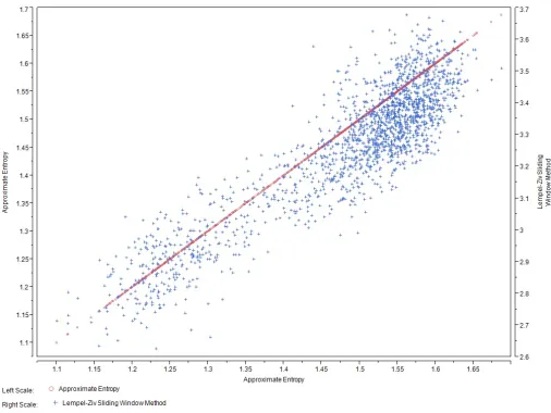
Last, we study the relationship between Approximate Entropy and Shannon Entropy, and propose the adaptive Shannon Entropy approximation methods (e.g., Lempel-Ziv sliding window method) as an alternative approach to quantify the regularity of data. The new approach has the advantage of adaptively choosing the order of regularity.

Degree Type

Dissertation

Degree Name

Doctor of Philosophy (PhD)

Graduate Group

Applied Mathematics

First Advisor

Alexander Rakhlin

Second Advisor

Abraham J. Wyner

Subject Categories

(3)

PREDICTABLE SEQUENCES

AND COMPETING WITH STRATEGIES

Wei Han

A DISSERTATION

in

Applied Mathematics and Computational Science

Presented to the Faculties of the University of Pennsylvania in Partial

Fulfillment of the Requirements for the Degree of Doctor of Philosophy

2013

Supervisor of Dissertation

Co-Supervisor of Dissertation

Alexander Rakhlin

Abraham J. Wyner

Assistant Professor of Statistics

Professor of Statistics

Graduate Group Chairperson

Charles L. Epstein

Thomas A. Scott Professor of Mathematics

Dissertation Committee:

Alexander Rakhlin, Assistant Professor of Statistics

Abraham J. Wyner, Professor of Statistics

(4)

Acknowledgements

It seems like yesterday that I arrived on the beautiful campus of the University of Pennsylvania, and it is hard to believe that four wonderful years have already passed. With memories everywhere across the campus, I owe thanks to many people in many ways.

I would like to express my deepest appreciation to all of my wonderful profes-sors. Thanks to Professor Charles L. Epstein for accepting me to The Graduate Group in Applied Mathematics and Computational Science (AMCS). That marked the beginning of all the memories. Thanks also to Professor Abraham J. Wyner for introducing me to the field of statistics and to the Wharton Statistics Department and many interesting projects. I would also like to extend my appreciation to Pro-fessor Alexander Rakhlin for introducing me to the field of online learning, and for his support and encouragement throughout my research. Karthik Sridharan offered many brilliant and inspiring ideas, and contributed greatly to my research. Profes-sor Dean Foster served on my thesis committee, and provided extremely valuable career advice. Many thanks, as well, to all of the great professors who instructed me during my twenty courses at Penn.

I could not have completed this program without the generous financial support of several professors and departments at the University of Pennsylvania. Thanks to Professor Charles L. Epstein, Professor Max Kelz, Professor Alexander Rakhlin, Department of Mathematics, AMCS and the Wharton Statistics Department.

Furthermore, I would like to express deep appreciation to all of the staff members of AMCS and the Wharton Statistics Department who helped me and made my life much easier. Thank you, Janet E. Burns, Audrey Masciocchi Caputo, Charlotte Merrick, Tanya Winder, Adam Greenberg, Carol Reich and Sarin Sieng.

In addition, thanks to all my friends, who took classes, shared offices and ideas, discussed problems, played bridge, travelled and tasted delicious food together.

(5)

ABSTRACT

PREDICTABLE SEQUENCES AND COMPETING WITH STRATEGIES

Wei Han

Alexander Rakhlin

Abraham J. Wyner

First, we study online learning with an extended notion of regret, which is defined

with respect to a set of strategies. We develop tools for analyzing the minimax

rates and deriving efficient learning algorithms in this scenario. While the

stan-dard methods for minimizing the usual notion of regret fail, through our analysis

we demonstrate the existence of regret-minimization methods that compete with

such sets of strategies as: autoregressive algorithms, strategies based on statistical

models, regularized least squares, and follow-the-regularized-leader strategies. In

several cases, we also derive efficient learning algorithms.

Then we study how online linear optimization competes with strategies while

benefiting from the predictable sequence. We analyze the minimax value of the

online linear optimization problem and develop algorithms that take advantage of

the predictable sequence and that guarantee performance compared to fixed actions.

Later, we extend the story to a model selection problem on multiple predictable

sequences. At the end, we re-analyze the problem from the perspective of dynamic

regret.

(6)

Entropy, and propose the adaptive Shannon Entropy approximation methods (e.g.,

Lempel-Ziv sliding window method) as an alternative approach to quantify the

regularity of data. The new approach has the advantage of adaptively choosing the

(7)

List of Tables

(10)

List of Figures

2.1 Mirror Descent . . . 8

4.1 Kalman Filter Scheme . . . 69

5.1 Approximate Entropy of Markov Model . . . 77

(11)

Chapter 1 Introduction

Online learning is a subfield of machine learning. There are two key points to dis-tinguish online learning from traditional machine learning algorithms and classical statistical methods. First, traditional machine learning algorithms and classical sta-tistical methods usually have strong assumptions about the data generating mecha-nism. For example, data come in the independent and identically distributed (i.i.d.) fashion, or data are generated from fixed distributions. However, these assumptions are not true in many environments. Online learning aims to avoid these strong as-sumptions, and to make sure that the algorithm works well, regardless of the data generating mechanism. Second, online learning focuses on the environment where new data constantly arrive over time, and real-time decisions are made at every step. Therefore, online learning algorithms emphasize computational efficiency.

Let us illustrate these ideas by a stock trading example. There are many stocks in the stock market. In each period, we only have enough resources to purchase a subset of these stocks. To keep the illustration simple, let us assume that we only have limited money and can only buy one single stock every day. The potential profit to be made from each stock varies on each day. At the end of each day, we observe profits of all the stocks in the stock market. The process of buying stocks and observing profit is repeated day after day. Before buying stocks, we have collected the profit information from previous days. We are interested in designing a trading strategy that maximizes our profit from buying stocks.

(12)

the profit of buying Stock B is consistently 1. According to the previous model, we will randomly choose Stock A or Stock B on the odd days, and consistently choose Stock A on the even days. However, it is wiser to choose Stock B on all even days. In the stock scenario, it is unreasonable to assume that the profits come from fixed distribution, and that the data generating process is highly non-stationary. Many factors influence the stock market. Also, other traders are constantly adjust-ing their tradadjust-ing strategies. This also affects stocks’ profit.

Therefore, what if we know little about the data generating process? What if it is unreasonable to make too many assumptions about the data generating process? Online learning aims to solve such a problem. The key philosophy of online learning is to remain agnostic about how data are generated. Algorithms in online learning guarantee the performance even in the worst situation, and the performance measure does not depend on specific data structures.

Since we make no assumption about how the data are generated, then there can always be one situation that we make very little profit regardless of the algorithm. If we just keep our eyes on the profit, there is no hope to make any progress. So, it is critical to define the performance measure for online learning algorithms.

There is an algorithm that make is as much profit as that made from constantly choosing the best stock over time. In the long run, the difference between the average profit of this algorithm and the average profit of the best stock, which is defined as regret, goes to zero. Furthermore, the regret vanishes at the rate of √

logN/T, where N is the size of the stock market. Or, if we collect the opinions fromN stock market experts, there exists an algorithm that earns almost the same profit as the best expert among theseN experts. It is interesting to notice that the rate of convergence depends on the size of the stock set or the size of the expert set. Regret is the key performance measure in online learning. Why should we only compete against fixed stocks / fixed experts? It only guarantees that the performance is as good as the best single stock / expert. If there is one stock / expert that performs well over this period of time, we are happy. But, what if none of these fixed stocks / expers performs well enough? If there is a strategy that can choose different stocks at different time based on revealed information, can we design an algorithm that performs as well as the best strategy?

Our research extends significantly the definition of regret, which is the most widely accepted performance measure in online leaning algorithms. Instead of com-peting with fixed actions, we are comcom-peting with strategies, which is defined as a set of functions that map from history to actions. As strategy is history-based, the regret competing with strategies provides a higher standard for performance measure of online learning algorithms.

(13)

with fixed actions / finite experts quickly converges to zero. However, if history-based strategies are considered, the size of the expert setN increases exponentially. For example, if we use history in the previous k steps, then there are 3k _strategies.

The longer the history is, the larger the strategy set is. It is interesting to note that many strategies are similar to each other, although the number of potential strategies is quite large. It is beneficial to group strategies according to the similarity of strategies. If we can group strategies according to their similarities, then the regret reduces even more quickly.

In Chapter 3, we define several complexity measures of strategies that dramat-ically reduce the number of “effective strategies”. Also, while earlier algorithms are only able to produce as much profit as fixed actions / finite experts, we de-rive novel algorithms that make as much profit as the best history-based strategy. Furthermore, we provide theoretical support for our algorithms.

Beyond our contribution to regret, we consider how to integrate outside infor-mation with the learning process. For example, there are seasonal factors that affect the stock market, and abnormal behaviors that occur around earnings announce-ments. In Chapter 4, the problem is formulated and efficient algorithms are derived to incorporate outside information.

(14)

Chapter 2 Online Learning

This chapter briefly describes the framework of online learning and related results in online learning. It follows closely to Alexander Rakhlin and Karthik Sridharan’s lecture notes of STAT928: Statistical Learning Theory and Sequential Prediction [16].

2.1 Framework of Online Learning

Suppose both the set of the learner’s choicesF and the set of the adversary’s choices Z are closed compact sets. The loss function`∶ F × Z →_R measures the quality of the learner’s choice. The learning framework is shown in the following table

Algorithm 1 Learning Framework

for t=1 to T do

We (The learner) pick(s) ft∈ F

The adversary picks zt∈ Z

We suffer loss `(ft, zt)

end for

Z can be also a set of experts. We, as the learner, choose to follow one expert’s choice at each step, according to experts’ historical performance. We can switch between experts, but can not mix experts’ choice at one single step. After the whole learning process, we may regret and say “I should follow the best expert if I know the sequence in advance”.

The difference between our cumulative loss and the cumulative loss of the best expert is used to evaluate the algorithm. The difference is defined as Regret and is formalized as

Reg_T(F) =

T ∑ t=1

`(ft, zt) −inf f∈F

T ∑ t=1

(15)

For the given pair (F,Z), the problem is called online learnable if there exists an algorithm that achieves sub-linear regret. One main problem in online learning is to analyze the learnability. Another problem is the construction of low-regret algorithms.

2.2 The Minimax Analysis

The minimax value of the online learning problem is defined as

VT(F) = inf

p1∈∆(F ) sup

z1∈Z

E f1∼p1

. . . inf

pT∈∆(F ) sup

zT∈Z

E fT∼pT

(∑T t=1

`(ft, zt) −inf f∈F

T ∑ t=1

`(f, zt)),

where ∆(F) includes all distributions over the set F. It is a powerful way to compress the process of online learning in one single formula.

The upper bound ofVT(F)guarantees the existence of learning algorithms that

perform as well as the best one in the comparator setF. The lower bound indicates that the adversary can cause that much damage regardless of learning algorithms. Also, the minimax regret gives us the access to analyze the learnability of more general online learning problem and to design learning algorithms.

Let us prepare several notations for further analysis. First, Rademacher random variablesrepresents a fair coin flip, and it equals to 1 or−1 with probability 0.5. Se-quences of Rademacher random variables are embedded in Sequential Rademacher Complexity [18] to capture the sequential nature of the online learning problem. Before we jump into the definition of Sequential Rademacher complexity, we first introduce the tree structure. A (complete binary) Z-valued tree z of depth T is a collection of functions z1, . . . ,zT such that zi ∶ {±1}i−1 → Z and z1 is a constant

function. A sequence of i.i.d. Rademacher random variables (1, . . . , T) defines a

path in on the tree z:

z1,z2(1),z3(1, 2), . . . ,zT(1, . . . , T−1).

Definition 2.2.1. The Sequential Rademacher Complexity of a function classF is defined as

Rseq

T (F) =sup

z E[

sup

f∈F

T ∑ t=1

t`(f,zt(1, . . . , t−1))],

where the outer supremum is taken over all Z-valued trees of depthT.

Furthermore, the value of the gameVT(F)is upper bounded by twice Sequential

Rademacher ComplexityRseq_T (F).

Theorem 2.2.2. [18]The minimax value of the online learning problem is bounded by

(16)

2.3 Algorithms in Online Learning

There are many interesting algorithms in online learning setting. I show two algo-rithms in this subsection, one is the Exponential Weights Algorithm and another is the Mirror Decent Algorithm.

2.3.1 Exponential Weights Algorithm

The Exponential Weights Algorithm focuses on the finite experts setting. For t = 1, . . . , T, the learner observes N difference choices f1

t, . . . , ftN ∈ F, chooses a

distributionptin aN−1 simplex, picks one choiceftit from theseN choices

accord-ing to the distribution pt, observe zt and suffers loss `(ftit, zt). The loss function `∶ F × Z →_R is convex in its first argument and takes value in [0,1]. The goal is to minimize the regret defined as

T ∑ t=1

E it∼qt

`(fit

t , zt) − inf i∈{1,...,N}

T ∑ t=1

`(f_ti, zt).

The Exponential Weights Algorithm randomly chooses one expert according to the historical performance. The probability of choosing one expert reduces if its historical performance is worse than other experts, otherwise, the probability increases. The Exponential Weights Algorithm achieves the optimal convergence rate of regret O(√TlnN), where N is the size of the expert set.

Algorithm 2 Exponential Weights Algorithm

Initialize: q1= (_N1, . . . ,_N1), η=

√

8 lnN T

for t=1 to T do

Sample it∼qt, and predict fit ∈ F

Observe zt and update

qt+1(i) ∝qt(i)e

−η`(fi,zt) _{for all} _i∈ {₁_{, . . . , N}}

end for

2.3.2 Mirror Descent Algorithm

Suppose both the set the learner’s choicesF and the outcome setZ are convex. At t=1, . . . , T, the learner chooses ft∈ F, observes zt∈ Z and suffers loss ⟨ft, zt⟩. The

goal is to minimize the regret defined as

T ∑ t=1

⟨ft, zt⟩ −inf f∈F

T ∑ t=1

(17)

Let us prepare several definitions for the algorithm. First, a function R is σ -strongly convex over F with respect to ∥ ⋅ ∥ if

R(a) ≥ R(b) + ⟨∇R(b), a−b⟩ +σ

2∥a−b∥

2

for all a, b ∈F. ∇R(b) can be replaced by any subgradient in ∂R(b) if R is non-differentiable. Then, the Bregman divergenceD(a, b)with respect to theσ-strongly convex function R is defined as

DR(a, b) = R(a) − R(b) − ⟨∆R(b), a−b⟩

and the convex conjugate of function R is defined as

R⋆(

u) =sup

a ⟨

u, a⟩ − R(a).

Algorithm 3 Mirror Descent Algorithm

Input: R is σ-strongly convex with respect to ∥ ⋅ ∥, learning rate η>0

for t=1 to T do

ft+1 =arg min

f∈F⟨

f, zt⟩ +η−1DR(f, ft)

or, equivalently,

˜

ft+1= ∇R

⋆(∇R(

ft) −ηzt)and ft+1 =arg min

f∈F D

R(f,f˜t+1)

end for

Mirror Descent, as a general version of Gradient Descent, focuses on online convex optimization and is computational efficient. Figure 2.1 illustrates three steps of the Mirror Descent Algorithm. First, the input ft in the primal space D is

mapped to the dual space by ∇R. Then, the gradient descent step −ηzt is done in

the dual spaceD⋆_{. At the end, the gradient descent update}∇R(_f

t)−ηztis mapped

back to the primal space D⋆ _by∇R⋆_.

2.4 The Algorithm Framework

(18)

ft

∇R(ft)

∇R⋆(∇R(_f

t) −ηzt) ∇R(_f

t) −ηzt ∇R

∇R⋆

−ηzt

Primal SpaceD Dual Space D⋆

(19)

Chapter 3 Competing with Strategies

In this chapter, we study the problem of online learning with a notion of regret de-fined with respect to a set of strategies. We develop tools for analyzing the minimax rates and for deriving regret-minimization algorithms in this scenario. While the standard methods for minimizing the usual notion of regret fail, through our anal-ysis we demonstrate existence of regret-minimization methods that compete with such sets of strategies as: autoregressive algorithms, strategies based on statistical models, regularized least squares, and follow the regularized leader strategies. In several cases we also derive efficient learning algorithms.

3.1 Introduction

The common criterion for evaluating an online learning algorithm is regret, that is the difference between the cumulative loss of the algorithm and the cumulative loss of the best fixed decision, chosen in hindsight. While much work has been done on understanding no-regret algorithms, such a definition of regret against a fixed decision often draws criticism: even if regret is small, the cumulative loss of a best

fixed action can be large, thus rendering the result uninteresting. To address this problem, various generalizations of the regret notion have been proposed, including regret with respect to the cost of a “slowly changing” compound decision. While being a step in the right direction, such definitions are still “static” in the sense that the decision of each compound comparator per step does not depend on the sequence of realized outcomes.

Arguably, a more interesting (and more difficult to deal with) notion is that of performing as well as a set ofstrategies (or, algorithms). A strategyπ is a sequence of functionsπt, for each time periodt, mapping the observed outcomes to the next

(20)

since some measure of the “effective number” of experts must play a role in the complexity of the problem: experts that predict similarly should not count as two independent ones. But what is a notion of closeness of two strategies? Imagine that we would like to develop an algorithm that incurs loss comparable to that of the best of an infinite family of strategies. To obtain such a statement, one may try to discretize the space of strategies and invoke the black-box experts method. As we show in this chapter, such an approach will not always work. Instead, we present a theoretical framework for the analysis of “competing against strategies” and for algorithmic development, based on the ideas in [18, 15].

The strategies considered in this chapter are termed “simulatable experts” in [3]. The authors also distinguish static and non-static experts. In particular, for static experts and absolute loss, [2] were able to show that problem complexity is governed by the geometry of the class of static experts as captured by its i.i.d. Rademacher averages. For nonstatic experts, however, the authors note that “unfortunately we do not have a characterization of the minimax regret by an empirical process”, due to the fact that the sequential nature of the online problems is at odds with the i.i.d.-based notions of classical empirical process theory. In recent years, however, a martingale generalization of empirical process theory has emerged, and these tools were shown to characterize learnability of online supervised learning, online convex optimization, and other scenarios [18, 1]. Yet, the machinery developed so far is not directly applicable to the case of general simulatable experts which can be viewed as mappings from an ever-growing set of histories to the space of actions. The goal of this chapter is precisely this: to extend the non-constructive as well as constructive techniques of [18, 15] to simulatable experts. We analyze a number of examples with the developed techniques, but we must admit that our work only scratches the surface. We can imagine further research developing methods that compete with interesting gradient descent methods (parametrized by step size choices), with Bayesian procedures (parametrized by choices of priors), and so on. We also note the connection to online algorithms, where one typically aims to prove a bound on the competitive ratio. Our results can be seen in that light as implying a competitive ratio of one.

(21)

“well specified”. To illustrate the point, we will exhibit an example where we can compete with the set of all Bayesian strategies (parametrized by priors). We then obtain a statement that we perform as well as the best of them without assuming that the model is correct.

This chapter is organized as follows. In Section 3.2, we extend the minimax analysis of online learning problems to the case of competing with a set of strategies. In Section 3.3, we show that it is possible to compete with a set of autoregressive strategies, and that the usual online linear optimization algorithms do not attain the optimal bounds. We then derive an optimal and computationally efficient algorithm for one of the proposed regimes. In Section 3.4 we describe the general idea of competing with statistical models that use sufficient statistics, and demonstrate an example of competing with a set of strategies parametrized by priors. For this example, we derive an optimal and efficient randomized algorithm. In Section 3.5, we turn to the question of competing with regularized least squares algorithms indexed by the choice of a shift and a regularization parameter. In Section 3.6, we consider online linear optimization and show that it is possible to compete with Follow the Regularized Leader methods parametrized by a shift and by a step size schedule.

3.2 Minimax Regret and Sequential Rademacher

Complexity

We consider the problem of online learning, or sequential prediction, that consists ofT rounds. At each timet= {1, . . . , T} ≜ [T], the learner makes a predictionft∈ F

and observes an outcome zt∈ Z, where F and Z are abstract sets of decisions and

outcomes. Let us fix a loss function ` ∶ F × Z ↦ _R that measures the quality of prediction. A strategy π= (πt)Tt=1 is a sequence of functions πt∶ Z

t−1 ↦ F _mapping

history of outcomes to a decision. Let Π denote a set of strategies. The regret with respect to Π is the difference between the cumulative loss of the player and the cumulative loss of the best strategy

Reg_T =

T ∑ t=1

`(ft, zt) −inf π∈Π

T ∑ t=1

`(πt(z1∶t−1), zt).

where we use the notation z1∶k≜ {z1, . . . , zk}. We now define the value of the game against a set Π of strategies as

VT(Π) ≜ inf q1∈Q

sup

z1∈Z

E f1∼q1

. . . inf

qT∈Q sup

zT∈Z

E fT∼qT

[Reg_T]

(22)

non-constructive bounds can be used as relaxations to derive an algorithm. This is the path we take in this chapter.

Let us describe an important variant of the above problem – that of supervised learning. Here, before making a real-valued prediction ˆyt on round t, the learner

observes side information xt ∈ X. Simultaneously, the actual outcome yt ∈ Y is

chosen by Nature. A strategy can therefore depend on the history x1∶t−1, yt−1 and the currentxt, and we write such strategies asπt(x1∶t, y1∶t−1), withπt∶ Xt×Yt

−1↦ Y_. Fix some loss function `(y, yˆ ). The value VS

T(Π)is then defined as

sup

x1 inf

q1∈∆(Y ) sup

y1∈Y

E ˆ y1∼q1

. . .sup

xT

inf

qT∈∆(Y ) sup

yT∈Y

E ˆ yT∼qT

[∑T t=1

`(yˆt, yt) −inf π∈Π

T ∑ t=1

`(πt(x1∶t, y1∶t−1), yt)]

To proceed, we need to define a notion of a tree. AZ-valued treezis a sequence of mappings {z1, . . . ,zT} with zt∶ {±1}t−1 ↦ Z. Throughout this chapter,t∈ {±1}

are i.i.d. Rademacher variables, and a realization of = (1, . . . , T) defines a path

on the tree, given by z1∶t() ≜ (z1(), . . . ,zt()) for any t ∈ [T]. We write zt() for

zt(1∶t−1). By convention, a sum ∑

b

a =0 fora>b and for simplicity assume that no

loss is suffered on the first round.

Definition 3.2.1. Sequential Rademacher complexity of the set Π of strategies is defined as

R(`,Π) ≜sup

w,zE

sup

π∈Π [∑T

t=1

t`(πt(w1(), . . . ,wt−1()),zt())] (3.2.1)

where the supremum is over two Z-valued trees z and wof depth T.

The w tree can be thought of as providing “history” while z providing “out-comes”. We shall use these names throughout this chapter. The reader might notice that in the above definition, the outcomes and history are decoupled. We now state the main result:

Theorem 3.2.2. The value of prediction problem with a setΠ of strategies is upper bounded as

VT(Π) ≤2R(`,Π)

While the statement is visually similar to those in [18, 19], it does not follow from these works. Indeed, the proof needs to deal with the additional complications stemming from the dependence of strategies on the history. Further, we provide the proof for a more general case when sequences z1, . . . , zT are not arbitrary but need

to satisfy constraints.

(23)

Specifically, the adversary at round t can only play xt that satisfy constraint Ct(z1, . . . , zt) = 1 where (C1, . . . , CT) is a predetermined sequence of constraints

with Ct∶ Zt↦ {0,1}. When each Ct is the function that is always 1 then we are in

the setting of the theorem statement where we play an unconstrained/worst case adversary. However the proof here allows us to even analyze constrained adversaries which come in handy in many cases. Following [19], a restriction P1∶T on the ad-versary is a sequenceP1, . . . ,PT of mappingsPt∶ Zt−1↦2P such thatPt(z1∶t−1)is a

convex subset of P for any z1∶t−1 ∈ Z

t−1_{. In the present proof we will only consider}

constrained adversaries, where Pt = ∆(Ct(z1∶t−1)) is the set of all distributions on the constrained subset

Ct(z1∶t−1) ≜ {z ∈ Z ∶Ct(z1, . . . , zt−1, z) =1}.

defined at time t via a binary constraint Ct ∶ Zt ↦ {0,1}. Notice that the set Ct(z1∶t−1)is the subset of Z from which the adversary is allowed to pick instancezt from given the history so far. It was shown in [19] that such constraints can model sequences with certain properties, such as slowly changing sequences, low-variance sequences, and so on. Let C be the set of Z-valued trees z such that for every ∈ {±1}T _and _t∈ [_T]_,

Ct(z1(), . . . ,zt()) =1,

that is, the set of trees such that the constraint is satisfied along any path. The statement we now prove is that the value of the prediction problem with respect to a set Π of strategies and against constrained adversaries (denoted by VT(Π,C1∶T)) is upper bounded by twice the sequential complexity

sup

w∈C,z

Esup π∈Π

T ∑ t=1

t`(πt(w1(), . . . ,wt−1())),zt()) (3.2.2)

where it is crucial that the w tree ranges over trees that respect the constraints along all paths, while z is allowed to be an arbitrary Z-valued tree. This fact that wrespects the constraints is the only difference with the original statement of Theorem 3.2.2.

For ease of notation we use ⟪ ⟫T_t₌₁ to denote repeated application of operators

such has sup or inf. For instance,⟪sup_a_t∈Ainfbt∈BErt∼P⟫

T

t=1[F(a1, b1, r1, ..., aT, bT, rT)] denotes sup_a_1∈_Ainf_b_1∈_B_Er1∼P. . .sup_a_T∈AinfbT∈BErT∼P[F(a1, b1, r1, ..., aT, bT, rT)].

(24)

constrained adversaries can be written as :

VT(Π,C1∶T) = ⟪inf

qt∈Q

sup

pt∈Pt(z1∶t−1)

E ft∼qt,zt∼pt⟫

T

t=1 [∑T

t=1

`(ft, zt) −inf π∈Π

`(πt(z1∶t−1), zt)]

= ⟪ sup

pt∈Pt(z1∶t−1)

E zt∼pt⟫

T

t=1 sup

π∈Π [∑T

t=1 inf

ft∈F

Ez′_t`(ft, zt′) −`(πt(z1∶t−1), zt)]

≤ ⟪ sup

pt∈Pt(z1∶t−1)

E zt∼pt⟫

T

t=1 sup

π∈Π [∑T

t=1

Ez_t′`(πt(z1∶t−1), z ′

t) −`(πt(z1∶t−1), zt)]

≤ ⟪ sup

pt∈Pt(z1∶t−1)

E zt,z′t∼pt⟫

T

t=1 sup

π∈Π [∑T

t=1

`(πt(z1∶t−1), z ′

t) −`(πt(z1∶t−1), zt)]

Let us now define the “selector function”χ∶ Z × Z × {±1} ↦ Z by

χ(z, z′

, ) = { z

′ _if = −₁

z if =1

In other words,χt selects betweenztand zt′depending on the sign of . We will use

the shorthand χt(t) ≜χ(zt, zt′, t)and χ1∶t(1∶t) ≜ (χ(z1, z ′

1, 1), . . . , χ(zt, zt′, t)). We

can then re-write the last statement as

⟪ sup

pt∈Pt(χ1∶t−1(1∶t−1))

E zt,z′_t∼pt

E t

⟫ T

t=1 sup

π∈Π [∑T

t=1

t(`(πt(χ1∶t−1(1∶t−1)), z ′

t)

−`(πt(χ1∶t−1(1∶t−1)), zt)) ] (3.2.3)

Afterzt,zt′andtare revealed,χt(t)is fixed and can only be eitherztorzt′. We

can remove the dependency of χt() on , and replace χt() by yt, which is either zt or zt′. Therefore, the last statement is upper bounded

sup

p1∈P1

E z1,z1′∼p1

E 1

sup

y1∈{z1,z′1} sup

p2∈P2(y1)

E z2,z2′∼p2

E 2

sup

y2∈{z2,z2′}

⋯ sup

yT−1∈{zT−1,z_T′₋₁}

sup

pT∈PT(y1∶T−1)

E zT,z′_T∼pT

E T

sup

π∈Π [∑T

t=1

t(`(πt(y1∶t−1), z ′

t) −`(πt(y1∶t−1), zt))]

= sup

z1,z′1∈C1

E 1

sup

y1∈{z1,z′1}

sup

z2,z2′∈C2(y1)

E 2

sup

y2∈{z2,z′2}

⋯ sup

yT−1∈{zT−1,z_T′₋₁}

sup

zT,z′_T∈CT(y1∶T−1)

E T

sup

π∈Π [∑T

t=1

t(`(πt(y1∶t−1), z ′

t) −`(πt(y1∶t−1), zt))]

Furthermore, as {zt, z′t} ∈ Ct(y1∶t−1) and yt ∈ {zt, z ′

t}, we can conclude that yt ∈ Ct(y1∶t−1). If we drop the constraint onzt and z

′

(25)

be yt∈ Ct(y1∶t−1), the last statement is upper bounded by

sup

z1,z1′∈Z

E 1

sup

y1∈C1 sup

z2,z′2∈Z

E 2

sup

y2∈C2(y1)

⋯ sup

yT−1∈CT−1(y1∶T−2) sup

zT,zT′∈Z E T

sup

π∈Π [∑T

t=1

t(`(πt(y1∶t−1), z ′

t) −`(πt(y1∶t−1), zt))]

=2 sup

z1∈Z E 1 sup y1∈C1 sup

z2∈Z

E 2

sup

y2∈C2(y1)

⋯ sup

yT−1∈CT−1(y1∶T−2) sup

zT∈Z

E T

sup

π∈Π [∑T

t=1

t`(πt(y1∶t−1), zt)]

(3.2.4)

since the two terms obtaining by splitting the supremum are the same. Next, we replace yt by wt+1 and add supremum over w1 at the beginning. Since w1 does not appear in the loss function, the last statement can be rewritten as

2 sup

w1∈Z sup

z1∈Z

E 1

sup

w2∈C1 sup

z2∈Z

E 2

⋯ sup

wT∈CT(w1∶T−1) sup

zT∈Z

E T

sup

π∈Π [∑T

t=1

t`(πt(w2∶t), zt)]

Now, we exchange the order of suprema and expectation and also maintain the constrains,

2 sup

w∈C′ sup

z E

sup

π∈Π [∑T

t=1

t`(πt(w2∶t()),zt())] = (∗)

In this step, we passed to the tree notation. Importantly, tree w does not range over all trees, but can only be a join of two trees in set C, i.e.

C′= {_w∶ ∀

1,w(1) ∈ C}

Define w∗ =_w(−₁) _and _w∗∗ =_w(+₁)_{, we can expend the expectation in} (∗) _with respect to 1 of the above expression by

sup

w∗∈C sup

z E2∶T

sup

π∈Π

[−`(π1(⋅),z1(⋅)) + T ∑ t=2

t`(πt(w∗1∶t−1()),zt())]

+ sup

w∗∗∈C sup

z E2∶T

sup

π∈Π

[`(π1(⋅),z1(⋅)) + T ∑ t=2

t`(πt(w∗∗1∶t−1()),zt())].

With the assumption that we do not suffer lose at the first round, which means `(π1(⋅),z1(⋅)) = 0, we can see that both terms achieve the suprema with the same w∗=_w∗∗_{. Therefore, the above expression can be rewrite as}

sup

w∈C sup

z E2∶T

sup

π∈Π [∑T

t=1

t`(πt(w1∶t−1()),zt())]

(26)

As we show below, the sequential Rademacher complexity on the right-hand side allows us to analyze general non-static experts, thus addressing the question raised in [2]. As the first step, we can “erase” a Lipschitz loss function, leading to the sequential Rademacher complexity of Π without the loss and without the z tree:

R(Π) ≜sup

w

R(Π,w) ≜sup

w E

sup

π∈Π [∑T

t=1

tπt(w1∶t−1())]

For example, supposeZ = {0,1}, the loss function is the indicator loss, and strategies have potentially dependence on the full history. Then one can verify that

sup

w,zE

sup

π∈Πk [∑T

t=1

t1{πt(w1∶t−1()) ≠zt()}]

=sup

w,zE

sup

π∈Πk [∑T

t=1

t(πt(w1∶t−1())(1−2zt()) +zt())] =R(Π) (3.2.5)

The same result holds when F = [0,1] and ` is the absolute loss. The process of “erasing the loss” (or, contraction) extends quite nicely to problems of supervised learning. Let us state the second main result:

Theorem 3.2.3. Suppose the loss function `∶ Y × Y ↦_R is convex and L-Lipschitz in the first argument, and let Y = [−1,1]. Then

VS

T(Π) ≤2Lsup

x,y E

sup

π∈Π [∑T

t=1

tπt(x1∶t(),y1∶t−1())]

where (x1∶t(),y1∶t−1()) naturally takes place of w1∶t−1() in Theorem 3.2.2.

Fur-ther, if Y = [−1,1] and `(y, yˆ ) = ∣yˆ−y∣,

VS

T(Π) ≥sup

x E

sup

π∈Π [∑T

t=1

tπt(x1∶t(), 1∶t−1)].

Proof. By convexity of the loss,

⟪sup

xt∈X inf

qt∈∆(Y ) sup

yt∈Y

E ˆ yt∼qt

⟫ T

t=1 [∑T

t=1

`(yˆt, yt) −inf π∈Π

T ∑ t=1

`(πt(x1∶t, y1∶t−1), yt)]

≤ ⟪sup

xt∈X inf

qt∈∆(Y ) sup

yt∈Y

E ˆ yt∼qt

⟫ T

t=1 sup

π∈Π [∑T

t=1 `′(

ˆ

yt, yt)(yˆt−πt(x1∶t, y1∶t−1))]

≤ ⟪sup

xt∈X inf

qt∈∆(Y ) sup

yt∈Y

E ˆ yt∼qt

sup

st∈[−L,L] ⟫

T

t=1 sup

π∈Π [∑T

t=1

st(yˆt−πt(x1∶t, y1∶t−1))]

(27)

notation, and it is understood that st’s range over [−L, L], while yt,yˆt overY and xt’s overX. Now, by Jensen’s inequality, we pass to an upper bound by exchanging Eˆyt and supyt∈Y:

⟪sup

xt

inf

qt∈∆(Y )

E ˆ yt∼qt

sup yt sup st ⟫ T

t=1 sup

π∈Π [∑T

t=1

= ⟪sup

xt

inf

ˆ yt∈Y

sup

yt,st

⟫ T

t=1 sup

π∈Π [∑T

t=1

Consider the last step, assuming all the other variables fixed:

sup xT inf ˆ yT sup

yT,sT

sup

π∈Π [∑T

t=1

=sup xT inf ˆ yT sup

pT∈∆(Y ×[−L,L])

E

(yT,sT)∼pT

sup

π∈Π [∑T

t=1

where the distributionpT ranges over all distributions on Y × [−L, L]. Now observe

that the function inside the infimum is convex in ˆyT, and the function inside suppT

is linear in the distribution pT. Hence, we can appeal to the minimax theorem,

obtaining equality of the last expression to

sup

xT

sup

pT∈∆(Y ×[−L,L]) inf

ˆ yT

E

(yT,sT)∼pT

[∑T t=1

styˆt−inf π∈Π

T ∑ t=1

stπt(x1∶t, y1∶t−1))]

=T∑−1 t=1

styˆt+sup xT sup pT inf ˆ yT E

(yT,sT)∼pT

[sTyˆT −inf π∈Π

T ∑ t=1

=T∑−1 t=1

styˆt+sup xT sup pT [inf ˆ yT ( E

(yT,sT)∼pT

sT)yˆT − E

(yT,sT)∼pT

inf

π∈Π

T ∑ t=1

=T∑−1 t=1

styˆt+sup xT

sup

pT E

(yT,sT)∼pT

[inf

ˆ yT

( E

(yT,sT)∼pT

sT)yˆT −inf π∈Π

T ∑ t=1

We can now upper bound the choice of ˆyT by that given by πT, yielding an upper

bound

T−1 ∑ t=1

styˆt+ sup xT,pT

E

(yT,sT)∼pT

sup π∈Π [inf ˆ yT ( E

(yT,sT)∼pT

sT)yˆT − T ∑ t=1

=T∑−1 t=1

styˆt+ sup xT,pT

E

(yT,sT) ∼pT

sup π∈Π ⎡⎢ ⎢⎢ ⎢⎢ ⎣ ⎛ ⎜ ⎝(y_T′E,s′_T)

∼pT

s′

T −sT ⎞ ⎟

⎠πT(x1∶T, y1∶T−1) − T−1

∑ t=1

(28)

The resulting upper bound is therefore

VS

T(Π) ≤ ⟪sup xt,pt

E

(yt,st)∼pt

⟫ T

t=1 sup

π∈Π [∑T

t=1

( E

(y′_t,s′_t)∼pt

s′

t−st)πt(x1∶t, y1∶t−1)]

≤ ⟪sup

xt,pt E

(yt,st)∼pt (y′_t,s′_t)∼pt

⟫ T

t=1 sup

π∈Π [∑T

t=1 (s′

t−st)πt(x1∶t, y1∶t−1)]

= ⟪sup

xt,pt E

(yt,st)∼pt (y′_t,s′_t)∼pt

E t

⟫ T

t=1 sup

π∈Π [∑T

t=1

t(s′t−st)πt(x1∶t, y1∶t−1)]

≤ ⟪sup

xt

sup (yt,st)

(y′ t,s′t)

E t

⟫ T

t=1 sup

π∈Π [∑T

t=1

≤ ⟪sup

xt,yt

sup

s′_t,st E t

⟫ T

t=1 sup

π∈Π [∑T

t=1

≤2⟪sup

xt,yt

sup

st∈[−L,L]

E t

⟫ T

t=1 sup

π∈Π [∑T

t=1

tstπt(x1∶t, y1∶t−1)]

Since the expression is convex in eachst, we can replace the range ofst by{−L, L},

or, equivalently,

VS

T(Π) ≤2L⟪sup xt,yt

sup

st∈{−1,1}

E t

⟫ T

t=1 sup

π∈Π [∑T

t=1

tstπt(x1∶t, y1∶t−1)] (3.2.6)

Now consider any arbitrary function ψ∶ {±1} ↦_R, we have that

sup

s∈{±1}

E[ψ(s⋅)] = sup s∈{±1}

1

2(ψ(+s) +ψ(−s)) = 1

2(ψ(+1) +ψ(−1)) =E[ψ()]

Since in Equation (3.2.6), for each t, st and t appear together as t⋅st using the

above equation repeatedly, we conclude that

VS

T(Π) ≤2L⟪sup xt,yt

E t

⟫ T

t=1 sup

π∈Π [∑T

t=1

tπt(x1∶t, y1∶t−1)]

=2Lsup

x,y E

sup

π∈Π [∑T

t=1

tπt(x1∶t(),y1∶t−1())]

The lower bound is obtained by the same argument as in [18].

(29)

Example 3.2.4 (History-independent strategies). Let πf ∈ _{Π be constant}

history-independent strategiesπ₁f =. . .=π_Tf =f∈ F. Then (3.2.1) recovers the definition of sequential Rademacher complexity in [18].

Example 3.2.5 (Static experts). For static experts, each strategy π is a predeter-mined sequence of outcomes, and we may therefore associate each π with a vector in ZT_{. A direct consequence of Theorem 3.2.3 for any convex} _L_{-Lipschitz loss is}

that

V(Π) ≤2L_Esup π∈Π

[∑T t=1

tπt]

which is simply the classical i.i.d. Rademacher averages. For the case of F = [0,1], Z = {0,1}, and the absolute loss, this is the result of [2].

Example 3.2.6 (Finite-order Markov strategies). Let Πk _{be a set of strategies that}

only depend on the k most recent outcomes to determine the next move. Theo-rem 3.2.2 implies that the value of the game is upper bounded as

V(Πk) ≤_{2 sup}

w,zEsupπ∈Πk[∑

T

t=1t`(πt(wt−k(), . . . ,wt−1()),zt())]

Now, suppose that Z is a finite set, of cardinality s. Then there are effectively ssk

strategies π. The bound on the sequential Rademacher complexity then scales as √

2sk_log(_s)_T_{, recovering the result of [7] (see [3, Cor. 8.2]).}

In addition to providing an understanding of minimax regret against a set of strategies, sequential Rademacher complexity can serve as a starting point for al-gorithmic development. As shown in [15], any admissible relaxation can be used to define a succinct algorithm with a regret guarantee. For the setting of this chapter, this means the following. Let Rel∶ Zt↦

R, for each t, be a collection of functions

satisfying two conditions:

∀t, inf

qt∈Q sup

zt∈Z

{ E

ft∼qt

`(ft, zt) +Rel(z1∶t)} ≤Rel(z1∶t−1),

and −inf

π∈Π

T ∑ t=1

`(πt(z1∶t−1), zt) ≤Rel(z1∶T) .

Then we say that the relaxation is admissible. It is then easy to show that regret of any algorithm that ensures above inequalities is bounded by Rel({}).

Theorem 3.2.7. The conditional sequential Rademacher complexity with respect to

Π

R(`,Π∣z1, . . . , zt)

≜sup

z,wt+E1∶T

sup

π∈Π [2

T ∑ s=t+1

s`(πs((z1∶t,w1∶s−t−1()),zs−t()) −

t ∑ s=1

`(πs(z1∶s−1), zs)]

(30)

Proof. Denote Lt(π) = ∑ts=1`(πs(z1∶s−1), zs). The first step of the proof is an appli-cation of the minimax theorem (we assume the necessary conditions hold):

inf

qt∈∆(F ) sup

zt∈Z

{ E

ft∼qt[

`(ft, zt)]

+sup

z,wt+E1∶T

sup

π∈Π [2

T ∑ s=t+1

s`(πs((z1∶t,w1∶s−t−1()),zs−t()) −Lt(π)]}

= sup

pt∈∆(Z ) inf

ft∈F {_zE

t∼pt[

`(ft, zt)]

+_zE t∼pt

sup

z,wt+E1∶T

sup

π∈Π [2

T ∑ s=t+1

s`(πs((z1∶t,w1∶s−t−1()),zs−t()) −Lt(π)]}

For any pt∈∆(Z), the infimum over ft of the above expression is equal to

E zt∼pt

sup

z,w t+E1∶T

sup

π∈Π [2

T ∑ s=t+1

s`(πs((z1∶t,w1∶s−t−1()),zs−t()) −Lt−1(π)

+inf

ft∈F

E zt∼pt[

`(ft, zt)] −`(πt(z1∶t−1), zt)]

≤ E

zt∼pt

sup

z,wtE+1∶T

sup

π∈Π [2

T ∑ s=t+1

s`(πs((z1∶t,w1∶s−t−1()),zs−t()) −Lt−1(π)

+ E

zt∼pt

[`(πt(z1∶t−1), zt)] −`(πt(z1∶t−1), zt)]

≤ E

zt,z′t∼pt

sup

z,wt+E1∶T

sup

π∈Π [2

T ∑ s=t+1

s`(πs((z1∶t,w1∶s−t−1()),zs−t()) −Lt−1(π)

+`(πt(z1∶t−1), z ′

t) −`(πt(z1∶t−1), zt)]

We now argue that the independent zt and zt′ have the same distribution pt, and

thus we can introduce a random sign t. The above expression then equals to

E zt,zt′∼pt

E t

sup

z,wt+E1∶T

sup

π∈Π [2

T ∑ s=t+1

s`(πs((z1∶t−1, χt(t),w1∶s−t−1()),zs−t())

−Lt−1(π) +t(`(πt(z1∶t−1), χt(−t))) −`(πt(z1∶t−1), χt(t)))]

≤ E

zt,zt′∼pt

sup

z′′,z′′′Et

sup

z,wtE+1∶T

sup

π∈Π [2

T ∑ s=t+1

s`(πs((z1∶t−1, χt(t),w1∶s−t−1()),zs−t())

−Lt−1(π) +t(`(πt(z1∶t−1), z ′′

t) −`(πt(z1∶t−1), z ′′′

(31)

Splitting the resulting expression into two parts, we arrive at the upper bound of

2 _E

zt,z′t∼pt

sup

z′′ Et

sup

z,wt+E1∶T

sup

π∈Π [ ∑T

s=t+1

s`(πs((z1∶t−1, χt(t),w1∶s−t−1()),zs−t())

−1

2Lt−1(π) +t`(πt(z1∶t−1), z ′′

t)]

≤ sup

z,z′,z′′Et

sup

z,wt+E1∶T

sup

π∈Π [ ∑T

s=t+1

2s`(πs((z1∶t−1, χt(t),w1∶s−t−1()),zs−t())

−Lt−1(π) +t`(πt(z1∶t−1), z ′′

t)] ≤RT(Π∣z1, . . . , zt−1).

The first inequality is true as we upper bounded the expectation by the supremum. The last inequality is easy to verify, as we are effectively filling in a root zt and z′t

for the two subtrees, for t= +1 andt= −1, respectively, and jointing the two trees

with a ∅ root.

One can see that the proof of admissibility corresponds to one step minimax swap and symmetrization in the proof of [18]. In contrast, in the latter chapter, all T minimax swaps are performed at once, followed byT symmetrization steps.

Conditional sequential Rademacher complexity can therefore be used as a start-ing point for possibly derivstart-ing computationally attractive algorithms, as shown throughout this chapter.

We may now define covering numbers for the set Π of strategies over the his-tory trees. The development is a straightforward modification of the notions we developed in [18], where we replace “any tree x” with a tree of histories w1∶t−1.

Definition 3.2.8. A set V of _R-valued trees is an α-cover (with respect to `p) of

a set of strategies Π on an Z∗_{-valued history tree} _w _if

∀π∈Π, ∀∈ {±1}T_, ∃_v∈_V _s.t. (1 T ∑

T

t=1∣πt(w1∶t−1()) −vt()∣p)

1/p ≤α .

(3.2.7)

An α-covering number Np(Π,w, α) is the size of the smallest α-cover.

For supervised learning, (x1∶t(),y1∶t−1())takes place ofw1∶t−1(). Now, for any history treew, sequential Rademacher averages of a class of[−1,1]-valued strategies Π satisfy

R(Π,w) ≤inf

α≥0

{αT +√2 logN1(Π,w, α)T}

and the Dudley entropy integral type bound also holds:

R(Π,w) ≤inf

α≥0

{4αT+12√T_∫

1

α √

(32)

In particular, this bound should be compared with Theorem 7 in [2], which employs a covering number in terms of a pointwise metric between strategies that requires closeness forall histories and all time steps. Second, the results of [2] for real-valued prediction require strategies to be bounded away from 0 and 1 by δ >0 and this restriction spoils the rates.

In the rest of this chapter, we show how the results of this section (a) yield proofs of existence of regret-minimization strategies with certain rates and (b) guide in the development of algorithms. For some of these examples, standard methods (such as Exponential Weights) come close to providing an optimal rate, while for others – fail miserably.

3.3 Competing with Autoregressive Strategies

In this section, we consider strategies that depend linearly on the past outcomes. To this end, we fix a set Θ⊂_Rk_{, for some}_k>_{0, and parametrize the set of strategies}

as

ΠΘ= {πθ∶πtθ(z1, . . . , zt−1) = ∑

k−1

i=0 θi+1zt−k+i, θ= (θ1, . . . , θk) ∈Θ}

For consistency of notation, we assume that the sequence of outcomes is padded with zeros for t ≤ 0. First, as an example where known methods can recover the correct rate, we consider the case of a constant look-back of size k. We then extend the study to cases where neither the regret behavior nor the algorithm is known in the literature, to the best of our knowledge.

3.3.1 Finite Look-Back

SupposeZ = F ⊂_Rd_are_`

2 unit balls, the loss is`(f, z) = ⟨f, z⟩, and Θ⊂Rk is also a

unit `2 ball. Denoting by W(t−k∶t−1)= [wt−k(), . . . ,wt−1()]a matrix with columns inZ,

R(`,ΠΘ) =sup

w,zE

sup

θ∈Θ [∑T

t=1

t⟨πθ(wt−k∶t−1()),zt()⟩] (3.3.1)

=sup

w,zE

sup

θ∈Θ [∑T

t=1

tzt()TW(t−k∶t−1)⋅θ]

=sup

w,zE∥

T ∑ t=1

tzt()TW(t−k∶t−1)∥ ≤ √

kT (3.3.2)

In fact, this bound against all strategies parametrized by Θ is achieved by the gradi-ent descgradi-ent (GD) method with the simple updateθt+1 =Proj_Θ(θt−η[zt−k, . . . , zt−1]

T zt)

where Proj_Θ is the Euclidean projection onto the set Θ. This can be seen by writing the loss as

⟨[zt−k, . . . , zt−1] ⋅θt, zt⟩ = ⟨θt,[zt−k, . . . , zt−1]

(33)

The regret of GD, ∑T_t=1⟨θt,[zt−k, . . . , zt−1]

T

zt⟩ −infθ∈Θ∑

T

t=1⟨θ,[zt−k, . . . , zt−1]

T zt⟩, is

precisely regret against strategies in Θ, and analysis of GD yields the rate in (3.3.1).

3.3.2 Full Dependence on History

The situation becomes less obvious when k =T and strategies depend on the full history. The regret bound in (3.3.1) is vacuous, and the question is whether a better bound can be proved, under some additional assumptions on Θ. Can such a bound be achieved by GD?

For simplicity, consider the case of F = Z = [−1,1], and assume that Θ = Bp(1) ⊂RT is a unit `p ball, for some p≥1. Since k=T, it is easier to re-index the

coordinates so that

πθ

t(z1∶t−1) = ∑

t−1

i=1θizi.

The sequential Rademacher complexity of the strategy class is

R(`,ΠΘ) =sup

w,zE

sup

θ∈Θ [∑T

t=1

tπθ(w1∶t−1()) ⋅zt()]

=sup

w,zE

sup

θ∈Θ [∑T

t=1 (t∑−1

i=1

θiwi())tzt()] .

Rearranging the terms, the last expression is equal to

sup

w,zE

sup

θ∈Θ [T∑−1

t=1

θtwt() ⋅ ( T ∑ i=t+1

izi())] ≤sup

w,zE[∥

w1∶T−1()∥_q⋅max

1≤t≤T∣

T ∑ i=t+1

izi()∣]

where q is the H¨older conjugate ofp. Observe that

sup

z E

sup

1≤t≤T ∣∑T

i=t

izi()∣ ≤sup

z E[∣

T ∑ i=1

izi()∣ + sup 1≤t≤T

∣t∑−1 i=1

izi()∣]

≤2 sup

z E

sup

1≤t≤T ∣∑t

i=1

izi()∣

Since {tzt() ∶ t =1, . . . , T} is a bounded martingale difference sequence, the last

term is of the order of O(√T). Now, suppose there is some β > 0 such that ∥w1∶T−1()∥_q ≤ T

β _{for all} _{. This assumption can be implemented if we consider}

constrained adversaries, where such `q-bound is required to hold for any prefix

w1∶t()of history (In Appendix, we prove Theorem 3.2.2 for the case of constrained sequences). Then R(`,ΠΘ) ≤C⋅Tβ+1/2 for some constant C. We now compare the

rate of convergence of sequential Rademacher and the rate of the mirror descent algorithm for different settings of q in Table 3.1. If ∥θ∥p ≤ 1 and ∥w∥q ≤ Tβ for q≥2, the convergence rate of mirror descent with Legendre function F(θ) = 1₂∥θ∥2 p

(34)

Θ w1∶T sequential Radem. rate Mirror descent rate B1(1) ∥w1∶T−1∥∞≤1

√

T √T logT

q≥2 Bp(1) ∥w1∶T−1∥q≤Tβ Tβ

+1/2 √_q−₁_Tβ+1/2

B2(1) ∥w1∶T−1∥2≤T

β _Tβ+1/2 _Tβ+1/2

1≤q≤2 Bp(1) ∥w1∶T−1∥q≤Tβ Tβ

+1/2 _Tβ+1/q

B∞(1) ∥w1∶T−1∥1≤Tβ Tβ

+1/2 _T

Table 3.1: Comparison of the rates of convergence (up to constant factors)

We observe that mirror descent, which is known to be optimal for online linear optimization, and which gives the correct rate for the case of bounded look-back strategies, in several regimes fails to yield the correct rate for more general linearly parametrized strategies. Even in the most basic regime where Θ is a unit `1 ball

and the sequence of data is not constrained (other thanZ = [−1,1]), there is a gap of √logT between the Rademacher bound and the guarantee of mirror descent. Is there an algorithm that removes this factor?

3.3.3 Algorithms for

Θ

=

B

1

(

1 )

For the example considered in the previous section, with F = Z = [−1,1] and Θ = B1(1), the conditional sequential Rademacher complexity of Theorem 3.2.7

becomes

RT(Π∣z1, . . . , zt) =sup

z,wt+E1∶T

sup

π∈Π [2

T ∑ s=t+1

sπs(z1∶t,w1∶s−t−1()) ⋅zs() −

t ∑ s=1

πs(z1∶s−1) ⋅zs]

≤sup

w t+E1∶T

sup

π∈Π [2

T ∑ s=t+1

sπs(z1∶t,w1∶s−t−1()) −

t ∑ s=1

zsπs(z1∶s−1)]

where the z tree is “erased”, as at the end of the proof of Theorem 3.2.3. Define as() =2s for s>t and −zs otherwise; bi() =wi() for i>t and zi otherwise. We

can then simply write

sup

w t+E1∶T

sup

θ∈Θ [∑T

s=1 as()

s−1 ∑ i=1

θibi()]

=sup

w tE+1∶T

sup

θ∈Θ [T∑−1

s=1

θsbs() T ∑ i=s+1

ai()]

≤ E

t+1∶T

max

1≤s≤T∣

T ∑ i=s

ai()∣

which we may use as a relaxation:

Lemma 3.3.1. Define at

s() =2s for s>t, and −zs otherwise. Then,

Rel(z1∶t) =Et+1∶Tmax1≤s≤T∣∑

T i=sa

(35)

is an admissible relaxation.

Proof. The first step of the proof is an application of the minimax theorem (we assume the necessary conditions hold):

inf

qt∈∆(F ) sup

zt∈Z

{ E

ft∼qt

ft⋅zt+ E t+1∶T

max

1≤s≤T∣

T ∑ i=s

at i()∣}

= sup

pt∈∆(Z ) inf

ft∈F

{ft⋅ E zt∼pt

zt+ E zt∼pttE+1∶T

max

1≤s≤T∣

T ∑ i=s

at_i()∣}

− ∣_zE t∼pt

zt∣ + E zt∼pt_t₊E₁_∶_T

max{max

s>t ∣

T ∑ i=s

at_i()∣,max

s≤t ∣

T ∑ i=s

at_i()∣}

≤_zE t∼pt_tE₊₁_∶_T

max{max

s>t ∣

T ∑ i=s

at_i()∣,max

s≤t ∣

T ∑ i=s

at_i() + _E z′_t∼pt

z′

t∣}

≤ E

zt,z′_t∼ptt+E1∶T

max{max

s>t ∣

T ∑ i=s

at_i()∣,max

s≤t ∣ ∑

i≥s,i≠t

at_i() + (z′

t−zt)∣}

We now argue that the independent zt and zt′ have the same distribution pt, and

E zt,zt′∼ptEt∶T

max{max

s>t ∣

T ∑ i=s

at_i()∣,max

s≤t ∣ ∑

i≥s,i≠t

at_i() +t(zt′−zt)∣}

≤_zE t∼ptE_t_∶_T

max{max

s>t ∣

T ∑ i=s

at_i()∣,max

s≤t ∣ ∑

i≥s,i≠t

at_i() +2tzt∣}

Now, the supremum over pt is achieved at a delta distribution, yielding an upper

bound

sup

zt∈[−1,1]

E t∶T

max{max

s>t ∣

T ∑ i=s

at

i()∣,max_s

≤t ∣ ∑

i≥s,i≠t at

i() +2tzt∣}

≤ E

t∶T

max{max

s>t ∣

T ∑ i=s

at_i()∣,max

s≤t ∣ ∑

i≥s,i≠t

at_i() +2t∣}

= E

t∶T

max

1≤s≤T∣

T ∑ i=s

at−1

i ()∣

With this relaxation, the following method attains O(√T)regret: prediction at step t is

qt=argmin q∈[−1,1]

sup

zt∈{±1}

{ E

ft∼q

ft⋅zt+Et+1∶T max 1≤s≤T∣

T ∑ i=s

(36)

where the sup over zt∈ [−1,1]is achieved at {±1} due to convexity. Following [15],

we can also derive randomized algorithms, which can be viewed as “randomized playout” generalizations of the Follow the Perturbed Leader algorithm.

Lemma 3.3.2. Consider the randomized strategy where at round t we first draw

t+1, . . . , T uniformly at random and then further draw our moveftaccording to the

distribution

qt() =argmin q∈[−1,1]

sup_z_t∈{−1,1}{Eft∼qft⋅zt+max1≤s≤T∣∑

T i=sa

t i()∣}

=1

2( max{maxs=1,...,t∣− ∑

t−1

i=szi+1+2∑

T

i=t+1i∣ , maxs=t+1,...,T∣2∑

T i=si∣} −max{maxs=1,...,t∣− ∑

t−1

i=szi−1+2∑

T

i=t+1i∣ , maxs=t+1,...,T∣2∑

T i=si∣})

The expected regret of this randomized strategy is upper bounded by sequential Rademacher complexity: _E[Reg_T] ≤2RT(Π), which was shown to be O(

√

T) (see Table 3.1). Proof. Let qt be the randomized strategy where we draw t+1, . . . , T uniformly at random and pick

qt() =argmin q∈[−1,1]

sup

zt∈{−1,1}

{ E

ft∼q

ft⋅zt+max 1≤s≤T∣

T ∑ i=s

at_i()∣} (3.3.3)

Then,

sup

zt∈{−1,1}

{ E

ft∼qt

T ∑ i=s

at i()∣}

= sup

zt∈{−1,1}

{Et+1∶T E ft∼qt()

T ∑ i=s

at_i()∣}

≤Et+1∶T[sup zt

{ E

ft∼qt()

T ∑ i=s

at_i()∣}]

=Et+1∶T[ inf qt∈∆(F )

sup

zt

{ E

ft∼qt

T ∑ i=s

at_i()∣}]

where the last step is due to the way we pick our predictor ft() given random

draw of ’s in Equation (3.3.3). We now apply the minimax theorem, yielding the following upper bound on the term above:

Et+1∶T[ sup pt∈∆(Z )

inf

ft

{ E

zt∼pt

ft⋅zt+ E zt∼pt

max

1≤s≤T∣

T ∑ i=s

(37)

This expression can be re-written as

E zt∼pt

inf

ft

{ E

z′_t∼pt

ft⋅zt′+max 1≤s≤T∣

T ∑ i=s

at i()∣}]

≤Et+1∶T[ sup pt∈∆(Z )

E zt∼pt

{− ∣ E

z′_t∼pt

z′

t∣ +max 1≤s≤T∣

T ∑ i=s

at_i()∣}]

E zt∼pt

max{max

s≤t ∣

T ∑ i=s

at_i() + _E z_t′∼pt

z′

t∣,max_s

>t ∣

T ∑ i=s

at_i()∣}]

E zt,z_t′∼pt

max{max

s≤t ∣

T ∑ i≥s,i≠t

at_i() + (z′

t−zt)∣,max s>t ∣

T ∑ i=s

at_i()∣}]

We now argue that the independent ztand zt′have the same distributionpt, and

E zt,z′t∼pt

E t

max{max

s≤t ∣

T ∑ i≥s,i≠t

at_i() +t(zt′−zt)∣,max s>t ∣

T ∑ i=s

at_i()∣}]

≤ E

t+1∶T

sup

zt∈{−1,1}

E t

max

1≤s≤T∣

T ∑ i=s

at−1

i ()∣ = E t∶T

max

1≤s≤T∣

T ∑ i=s

at−1

i ()∣

The time consuming parts of the above randomized method are to draw T −t random bits at roundt and to calculate the partial sums. However, we may replace Rademacher random variables by GaussianN (0,1)random variables and use known results on the distributions of extrema of a Brownian motion. To this end, define a Gaussian analogue of conditional sequential Rademacher complexity

GT(Π∣z1, . . . , zt)

=sup

z,wσtE+1∶T

sup

π∈Π [√2π

T ∑ s=t+1

σs`(πs((z1∶t,w1∶s−t−1()),zs−t()) −

t ∑ s=1

`(πs(z1∶s−1), zs)]

where σt ∼ N (0,1), and = (sign(σ1), . . . ,sign(σT)). For our example the O( √

T) bound can be shown for GT(Π) by calculating the expectation of the maximum

of Brownian motion. Proofs similar to Theorem 3.2.2 and Theorem 3.2.7 show that the conditional Gaussian complexity GT(Π∣z1, . . . , zt) is an upper bound on

RT(Π∣z1, . . . , zt)and is admissible.

Theorem 3.3.3. The conditional sequential Rademacher complexity with respect to

Π

GT(`,Π∣z1, . . . , zt)

≜sup

z,wσtE+1∶T

sup

π∈Π [√2π

T ∑ s=t+1

σs`(πs((z1∶t,w1∶s−t−1()),zs−t()) −

t ∑ s=1

`(πs(z1∶s−1), zs)]

(38)

Proof. Denote Lt(π) = ∑st=1`(πs(z1∶s−1), zs). Let c=Eσ∣σ∣ = √

2/π. The first step of the proof is an application of the minimax theorem (we assume the necessary conditions hold):

inf

qt∈∆(F ) sup

zt∈Z

{ E

ft∼qt[

`(ft, zt)]

+sup

z,wσtE+1∶T

sup π∈Π [2 c T ∑ s=t+1

σs`(πs((z1∶t,w1∶s−t−1()),zs−t()) −Lt(π)]}

= sup

pt∈∆(Z ) inf

ft∈F {_zE

t∼pt[

`(ft, zt)]

+_zE t∼pt

sup

z,w σtE+1∶T

σs`(πs((z1∶t,w1∶s−t−1()),zs−t()) −Lt(π)]}

E zt∼pt

sup

z,w σtE+1∶T

σs`(πs((z1∶t,w1∶s−t−1()),zs−t()) −Lt−1(π)

+inf

ft∈F

E zt∼pt[

`(ft, zt)] −`(πt(z1∶t−1), zt)]

≤ E

zt∼pt

sup

z,wσtE+1∶T

+ E

zt∼pt

[`(πt(z1∶t−1), zt)] −`(πt(z1∶t−1), zt)]

≤ E

zt,z′t∼pt

sup

z,wσtE+1∶T

sup

π∈Π

[2_c ∑T s=t+1

+`(πt(z1∶t−1), z ′

t) −`(πt(z1∶t−1), zt)]

We now argue that the independentztandzt′have the same distributionpt, and thus

we can introduce a gaussian random variable σt and a random sign t = sign(σt).

The above expression then equals to

E zt,z′t∼pt

E σt

sup

z,wσtE+1∶T

σs`(πs((z1∶t−1, χt(t),w1∶s−t−1()),zs−t()) −Lt−1(π)

+t(`(πt(z1∶t−1), χt(−t))) −`(πt(z1∶t−1), χt(t)))]

≤ E

zt,zt′∼pt E σt

sup

z,wσtE+1∶T

σs`(πs((z1∶t−1, χt(t),w1∶s−t−1()),zs−t()) −Lt−1(π)

+tE σt

∣σt

Predictable Sequences and Competing with Strategies

University of Pennsylvania

ScholarlyCommons

Predictable Sequences and Competing with

Strategies

Wei Han

Predictable Sequences and Competing with Strategies

PREDICTABLE SEQUENCES

AND COMPETING WITH STRATEGIES

Wei Han

A DISSERTATION

in

Applied Mathematics and Computational Science

Presented to the Faculties of the University of Pennsylvania in Partial

Fulfillment of the Requirements for the Degree of Doctor of Philosophy

2013

Supervisor of Dissertation

Co-Supervisor of Dissertation

Alexander Rakhlin

Abraham J. Wyner

Assistant Professor of Statistics

Professor of Statistics

Graduate Group Chairperson

Charles L. Epstein

Thomas A. Scott Professor of Mathematics

Dissertation Committee:

Alexander Rakhlin, Assistant Professor of Statistics

Abraham J. Wyner, Professor of Statistics

Acknowledgements

Contents

List of Tables

List of Figures

Chapter 1

Introduction

Chapter 2

Online Learning

2.1

Framework of Online Learning

2.2

The Minimax Analysis

2.3

Algorithms in Online Learning

2.3.1

Exponential Weights Algorithm

2.3.2

Mirror Descent Algorithm

2.4

The Algorithm Framework

Chapter 3

Competing with Strategies

3.1

Introduction

3.2

Minimax Regret and Sequential Rademacher

Complexity

3.3

Competing with Autoregressive Strategies

3.3.1

Finite Look-Back

3.3.2

Full Dependence on History

3.3.3

Algorithms for

Θ

=

B

(

1

)