Partial Information Framework: Basic Theory and Applications

(1)

University of Pennsylvania

ScholarlyCommons

Publicly Accessible Penn Dissertations

1-1-2016

Partial Information Framework: Basic Theory and

Applications

Ville Antton Satopää

University of Pennsylvania, [email protected]

Follow this and additional works at:http://repository.upenn.edu/edissertations

Part of theApplied Mathematics Commons,Mathematics Commons, and theStatistics and Probability Commons

This paper is posted at ScholarlyCommons.http://repository.upenn.edu/edissertations/1991

For more information, please [email protected].

Recommended Citation

Satopää, Ville Antton, "Partial Information Framework: Basic Theory and Applications" (2016).Publicly Accessible Penn Dissertations. 1991.

(2)

Partial Information Framework: Basic Theory and Applications

Abstract

Many real-world decisions depend on accurate predictions of some future outcome. In such cases the decision-maker often seeks to consult multiple people or/and models for their forecasts. These forecasts are then aggregated into a consensus that is inputted in the final decision-making process. Principled aggregation requires an understanding of why the forecasts are different. Historically, such forecast heterogeneity has been explained by measurement error. This dissertation, however, first shows that measurement error is not appropriate for modeling forecast heterogeneity and then introduces information diversity as a more appropriate yet fundamentally different alternative. Under information diversity differences in the forecasts stem purely from differences in the information that is used in the forecasts. This is made mathematically precise in a new modeling framework called the partial information framework. At its most general level, the partial information framework is a very reasonable model of multiple forecasts and hence offers an ideal platform for theoretical analysis. For one, it explains the empirical phenomenon known as extremization. This is a popular technique that often improves the out-of-sample performance of simple aggregators, such as the average or median, by transforming them directly away from the marginal mean of the outcome.

Unfortunately, the general framework is too abstract for practical applications. To apply the framework in practice one needs to choose a parametric distribution for the forecasts and outcome. This dissertation motivates and chooses the multivariate Gaussian distribution. The result, known as the Gaussian partial information model, is a very close yet practical specification of the framework. The optimal aggregator under the Gaussian model is shown to outperform the state-of-the-art measurement error aggregators on both synthetic and many different types of real-world forecasts.

Degree Type

Dissertation

Degree Name

Doctor of Philosophy (PhD)

Graduate Group

Statistics

First Advisor

Lyle H. Ungar

Second Advisor

Shane T. Jensen

Keywords

(3)

Subject Categories

(4)

PARTIAL INFORMATION

FRAMEWORK: BASIC THEORY AND

APPLICATIONS

Ville A. Satop¨a¨a

A DISSERTATION

in

Statistics

For the Graduate Group in

Managerial Science and Applied Economics

Presented to the Faculties of the University of Pennsylvania

in

Partial Fulfillment of the Requirements for the

Degree of Doctor of Philosophy

2016

Supervisor of Dissertation

Shane T. Jensen

Associate Professor of Statistics

Co-Supervisor of Dissertation

Lyle H. Ungar

Professor of Computer and Information Science

Graduate Group Chairperson

Eric Bradlow

K.P. Chao Professor, Marketing, Statistics and Education

Dissertation Committee

Shane T. Jensen, Associate Professor Lyle H. Ungar, Professor

Edward I. George, Professor

(5)

PARTIAL INFORMATION FRAMEWORK: BASIC THEORY AND APPLICATIONS

(6)

Dedication

This dissertation has been dedicated to my mother, whose love and support give me courage to take on anything, and to my father, who lives on as the inspiration in everything I do.

(7)

Acknowledgments

First and foremost, I would like to thank my family and friends whose unquestioning sup-port has allowed me to chase my dreams to the edge of the world and back again. Second, I would like to thank my thesis committee for all their mentoring and advice about research, life, and everything in between. Lastly, I would like to thank my two Ph.D. advisors for always having my back, for reminding me of the bigger picture when I was lost in the de-tails, and for making me a much better researcher. Thanks to them, I could not feel any better-equipped to begin my career as a professor.

(8)

ABSTRACT

PARTIAL INFORMATION FRAMEWORK:

BASIC THEORY AND APPLICATIONS

Ville A. Satop¨a¨a

Shane T. Jensen

Lyle H. Ungar

(9)

List of Tables

2.1 Out-of-sample accuracies of the competing aggregators . . . 32

3.1 Five-number summaries of our real-world data . . . 40

3.2 Frequencies of the self-reported expertise . . . 40

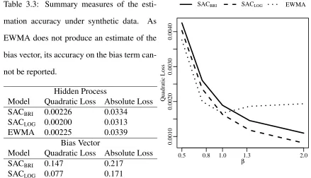
3.3 Summary measures of the estimation accuracy under synthetic data . . . 51

3.4 Brier Scores based on 10-fold cross-validation . . . 59

4.1 Average Brier scores with its three components . . . 95

5.1 Summary of the data across three time intervals . . . 126

6.1 Bayesian aggregation and expert predictions for individual states . . . 151

6.2 Squared error loss for aggregation procedures . . . 152

6.3 Some rows of ROC table . . . 153

7.1 Estimated parameter values under synthetic data . . . 171

7.2 The average quadratic loss under synthetic data . . . 173

7.3 Estimated parameter values under real-world data . . . 178

(12)

List of Figures

2.1 Aggregators under30synthetic problems and correct model . . . 23

2.2 Aggregators under100synthetic problems and correct model . . . 23

2.3 Aggregators under100synthetic problems and incorrect model . . . 26

2.4 Aggregators under69real-world problems . . . 30

2.5 Sensitivity to the choice ofa . . . 34

2.6 Optimal transformationaagainst self-reported expertise . . . 34

3.1 Probability forecasts for two IARPA events . . . 42

3.2 The marginal effect ofβon the average quadratic loss . . . 51

3.3 In- and out-of-sample calibration and sharpness . . . 61

3.4 Posterior distributions ofbj forj = 1, . . . ,5 . . . 63

4.1 Illustration of information distribution amongN forecasters . . . 83

4.2 Marginal distribution ofpi under different levels ofδi . . . 83

4.3 Levelplot of the extremization ratio . . . 90

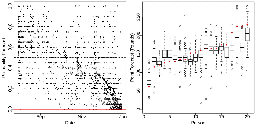
5.1 Probability forecasts of an IARPA event . . . 101

5.2 Point forecasts of the weights of20different people . . . 101

5.3 Average prediction accuracies of the competing probability aggregators . . 128

5.4 The estimatedΣfor the100GJP forecasters . . . 131

5.5 Average prediction accuracy of the competing real-valued aggregators . . . 134

5.6 The estimatedΣcov for the416CMU undergraduates . . . 134

6.1 Marginal distribution ofpj under different levels ofβ . . . 145

6.2 Comparisons of the aggregators’ behavior . . . 148

6.3 Illustration of two forecasters’ information partition . . . 149

6.4 DeSart predictions, Silver predictions, and Bayesian aggregation predictions 151 6.5 Predictions for the aggregators . . . 152

(13)

7.2 Out-of-sample reliability under no information overlap and synthetic data . 171 7.3 Out-of-sample reliability under high information overlap and synthetic data 171

7.4 Out-of-sample reliability of the individual models under real-world data . . 177

7.5 Out-of-sample reliability under no information overlap and real-world data 177 7.6 Out-of-sample reliability under high information overlap and real-world data 178 A.1 Summary comparison of the aggregators . . . 198

A.2 Estimation accuracy and the condition numbers . . . 215

A.3 Prediction accuracy under different values ofN andK . . . 217

A.4 Illustration a) for the proof . . . 224

(14)

1

Introduction

A new form of polling has emerged from the recent development of computer and social

networks; it is called prediction polling (Atanasov et al., 2015). In a prediction poll a group

of participants collectively make predictions about some future quantity of interest. For

instance, consider a policy maker who is interested in the probability of Brexit. Instead of

collecting data and aiming to build a statistical model, the policy-maker may reach out to

a group of European Union experts and ask them for their subjective probabilities of the

event. After this, the decision-maker must choose how to use the forecasts. The first idea

may be to simply follow the most accurate or informed forecaster’s advice. Unfortunately,

however, it is often not possible to know ex-ante who this forecaster is, and even if one

somehow could know, simply following a single forecaster’s advice would ignore

poten-tially a large amount of information that is being contributed by the rest of the forecasters.

Therefore a better option is to combine the forecasts into a single consensus forecast that

re-flects all forecasters’ information. Unfortunately, there are many ways one could combine

the predictions, and the final combination rule will largely determine the out-of-sample

performance of the consensus forecast.

The past literature has distinguished two general approaches to forecast aggregation:

1. Empirical. Overall, this approach is by far the more widely studied one. It is akin to

(15)

aggre-gators and within that class chooses the aggregator that performs the best over some

training set of past predictions on known outcomes. The chosen aggregator is then

used for combining any future predictions of unknown outcomes.

2. Model-based. This approach begins with a probability model of forecast

hetero-geneity, that is, the way the predictions differ from each other and the outcome. The

model-based aggregator is then the optimal aggregator under this assumed

outcome-forecast link. Note that applying the aggregator in practice may or may not involve

estimating some model parameters from the forecasts – but not from the outcomes.

Both of these approaches are important and serve somewhat different purposes. More

specifically, the empirical techniques are often simpler and work very well when one has

access to a training set that is representative of the future aggregation tasks. There are,

however, many forecasting applications where a training set is not available. For instance,

in prediction polling obtaining a training set would require a lot of time and effort on behalf

of the forecasters and polling agency. For this reason, many prediction polls do not yield

a training set. Instead, the participants are typically handed out a single questionnaire that

solicits their predictions about one or more future outcomes. Fortunately, the model-based

aggregation approach can be applied directly to the forecasts even when no knowledge

of the outcomes is available. Therefore the model-based approach is much more broadly

applicable than the empirical approach. Furthermore, the model-based aggregators are

based on theory which provides a clear direction for improvement. Of course, this all

comes at a cost. In particular, the model-based approach relies on modeling assumptions.

If these assumptions are no appropriate, the resulting aggregators are, unfortunately, only of

limited use. Therefore it is important to perform careful model evaluation of any proposed

model-based aggregators.

This dissertation was largely motivated by the lack of an appropriate framework for

(16)

fore-cast heterogeneity has been explained with measurement error: the forefore-casts are assumed

to be equal to the true outcome plus some mean zero idiosyncratic error. While this

as-sumption may make sense when modeling estimates arising from repeated applications

of a sensitive yet somewhat imprecise instrument, it is hardly reasonable when the

esti-mates arise from multiple, often widely different sources. Furthermore, the measurement

error based aggregators are different types of measures of central tendency such as the

(weighted) average or median. Unfortunately, such simple aggregators do not behave as if

they are collecting information from the different forecasters. To illustrate, consider a

pa-tient who is worried about his or her health and hence goes to the hospital. At the hospital

both a blood test and an MRI are taken. Both tests come back with no evidence of poor

health. Suppose there are two doctors who decide to look at the patient’s case: doctorsA

andB. DoctorAonly looks at the blood test results and provides a probability of0.9of the

patient being healthy. DoctorB, on the other hand, only looks at the MRI results but also

provides a probability of0.9of the patient being healthy. Now, the patient has two0.9s that

are based on very different information. How should they be aggregated? Surely, if one

were to see the good news both from the blood test and the MRI, one would be even more

convinced of the patient’s good health and hence predict something greater than 0.9. In

other words, in this simple example the combined evidence should yield a forecast

some-what greater than0.9. Unfortunately, however, all measures of central tendency aggregate

precisely to0.9. Therefore they fail to account for the doctors’ differing information sets

and hence cannot collect information from the different forecasters. Of course, this is only

a simple example. The result, however, is much more general than this. In fact, as will be

shown in Chapter 7, this result holds for any number of forecasters despite whether their

forecasts are equal or not.

In order to fix this shortcoming, it is necessary to revisit the fundamentals. In particular,

(17)

appropri-ate than measurement error and it should lead to aggregators that do behave as if they

were collecting information from the different forecasters. Such an alternative is precisely

what is introduced in this dissertation; it is calledinformation diversity. Under information

diversity, the differences in the predictions are fully explained by differences in the

infor-mation used by the respective forecasters. For instance, consider two forecasters predicting

the chances of some global crisis. One of these forecasters lives in USA and follows the

American news. The second forecaster, on the other hand, lives in Russia and reads the

Russian news. Given these descriptions, it is likely that the two forecasters have different

information and hence provide different predictions. This intuition is mathematically

for-malized in a new modeling framework called thepartial information framework. Overall,

the partial information framework is very general and can be applied to a broad range of

different forecasting applications, allowing the practitioner to construct application-specific

aggregators instead of always relying on the usual average and median. The partial

infor-mation aggregators also behave as if they collect inforinfor-mation from the forecasters and often

outperform the state-of-the-art measurement error aggregators in real-world applications.

Given that information diversity is a contribution at the root of statistical theory, it gives

rise to a large amount of new theory and methodology. This dissertation discusses several

such projects. In particular, each chapter is a separate paper discussing a different aspect

of the partial information framework. The chapters have been ordered chronologically in

the order they were written. The following enumeration briefly describes each chapter and

provides citations of the corresponding papers.

Chapter 2. Satop¨a¨a et al. (2014) introduces a new empirical aggregator for

prob-ability forecasts. Overall, the aggregator is very simply: it involves only a single

tuning parameter which determines how much the average log-odds forecast should

be extremized. Here extremization refers to the process of transforming a measure of

(18)

(typi-cally at0.5for probability forecasts) and closer to the nearest extreme (at0.0or1.0).

This extremizing aggregator is then shown to outperform simple measurement-error

aggregators on real-world predictions. Furthermore, the amount of extremization

was observed to decrease in the forecaster’s self-reported expertise.

Note:At this point the benefits of extremizing were merely an empirical observation.

In particular, it was not clear why it helps or how much extremization should be

performed.

Chapter 3. Satop¨a¨a et al. (2014)1 _{was largely motivated by the data collected by}

the Good Judgment Project (GJP) (Mellers et al., 2014). More specifically, the GJP

recruited 1,000s of experts to make probability forecasts of hundreds of future events

deemed important by the Intelligence Advanced Research Projects Activity (IARPA).

Each event was succeeded by a period of time during which the forecasters were

allowed to make predictions and update them if they felt that the likelihoods had

changed. Therefore each forecaster gave a time-series of predictions. To aggregate

such streams of forecasts, this paper develops an empirical aggregator that extremizes

and combines predictions over time. Furthermore, the amount of extremization is

al-lowed to vary across different self-reported expertise groups. Overall, the aggregator

outperforms classical exponentially-weighted aggregators on real-world predictions

from the GJP.

Note: Even though this paper contributes to a common forecasting setup where the

forecasters are allowed to update their forecasts over time, all methodology is

empir-ical and hence requires the decision-maker to conduct a rather large study in which

the forecasters are making and updating forecasts for multiple events. Also, given

that the aggregator is learned over a training set, the decision-maker must wait for

1_{This is the thesis for my Master of Arts in Statistics degree received in December 2014. It is included}

(19)

each of the events to be resolved. This illustrates the limitations of the empirical

ag-gregation approach. In some sense, the benefits of extremizing suggest a bias in the

underlying probability model, namely the measurement error model that motivates

the simple aggregators applied before extremization.

Chapter 4. Satop¨a¨a et al. (2015) introduces the partial information framework for

probability forecasts. The framework motivates two benchmarks for aggregation:

the oracular and revealed aggregators. The oracular aggregator has access to all

the details of the forecasters’ information and hence is only useful for theoretical

analysis. The revealed aggregator, on the other hand, can be used in practice as it

only depends on information revealed through the reported forecasts. As a practical

specification of the framework the first version of the Gaussian partial information

model is developed. This version describes full information by some closed interval.

Each forecaster then observes some Borel subset of this interval. The variance of the

forecast is the size of the corresponding Borel set, and the covariance between any

two forecasters is the size of the overlap between their Borel sets. This motivates

a structure for the covariance matrix that has to be in a convex set known as the

correlation polytope. In the paper the oracular aggregator under the Gaussian model

is used as benchmark to analyze the amount of required extremization under different

information structures. In particular, it is found that extremization increases in two

separate measures: the total amount of information and the amount of information

diversity among the forecasters. This motivates a spectrum of aggregators, ranging

from averaging (full information overlap) to summing (no information overlap).

Note:While information diversity is intuitively much more appealing than

measure-ment error, this paper was mainly theoretical and contained very little empirical

evi-dence in favor of information diversity. Furthermore, the focus was entirely on

(20)

information diversity is a much more general concept: it is an alternative to

measure-ment error and hence suggests a more general modeling framework.

Chapter 5. Satop¨a¨a et al. (2016) introduces information diversity as a general

alter-native to measurement error and shows how the partial information framework can

be used in practice to model different types of outcome-forecast pairs, such as

proba-bility forecasts of binary outcomes or real-valued forecasts of real-valued outcomes.

Such applications are made more tractable by modifying the Gaussian model. In

par-ticular, it turns out that applying the partial information framework in practice only

needs a choice of a parametric family of distributions for the outcome and forecasts

– nothing else. The multivariate Gaussian distribution here leads to our second

ver-sion of the Gaussian model. This time the form of the forecasts’ covariance matrix

is motivated solely by the general partial information framework instead of

overlap-ping Borel sets. Most importantly, however, the revised form is much more tractable

than the one introduced by the first version of the Gaussian model. The paper then

develops a procedure for estimating these covariance matrices and applies the

re-vised Gaussian model to two real-world applications. The analysis leads to several

observations. First, in both cases the revealed aggregator significantly outperforms

the state-of-the-art measurement error aggregators. Second, unlike the measurement

error aggregators, the revealed aggregator behaves as if it is collecting information

from the forecasters. Third, the estimated information structure aligns well with prior

knowledge about the forecasters’ information.

Note: This paper provides much empirical evidence in favor of information

diver-sity as the more important source of forecast heterogeneity. The estimation

pro-cedure therein, however, requires the forecasters to make predictions for multiple

related outcomes. Unfortunately, in many forecasting setups multiple outcomes are

(21)

information structure cannot be assumed to remain constant among them. Ideally,

one would have a partial information aggregator that can operate directly on a set of

forecasts of a single outcome.

Chapter 6.Ernst et al. (2016) introduces the notion of Bayes-Gaussian aggregation.

The motivation relies on previous applications that have inputted a point estimate

of the information structure to the revealed aggregator. Such plug-in aggregators,

however, can be unstable. To avoid this, a Bayes-Gaussian aggregator computes a

posterior-weighted mixture of the plug-in aggregators under all possible information

structures. In this paper a Bayes-Gaussian aggregator is developed for two

probabil-ity forecasts of a single event. To simplify the computations, each of the forecasters

is assumed to know half of the total information. Their information overlap, however,

is considered unknown and is analytically integrated out with respect to its posterior

distribution. The final form is a simple aggregator that is free of any model

parame-ters and hence can be applied directly to any two probability forecasts. Even though

the literature on Bayesian statistics offers many numerical procedures for

integra-tion, the model parameters here are integrated out analytically in order to arrive at

a closed-form aggregator. The hope is that such a simple closed-form encourages

practitioners to abandon the usual average and median aggregators.

Chapter 7. Satop¨a¨a and Ungar (2015) begins by proving and discussing some

gen-eral results under the partial information framework. For one, it makes the notion

of information collection precise: an information collector is a calibrated

aggrega-tor, as this shows that it is consistent with some information set about the outcome,

and its variance is at least as large as the maximum variance among the individual

forecasts. The paper then proceeds to show that the revealed aggregator does

col-lect information. In contrast, the weighted average of calibrated forecasts is shown

(22)

tendency generally reduce variance, these simple aggregators can be intuitively seen

to not collect information either. Furthermore, the weighted average tends to be too

close (as compared to the revealed aggregator) to the marginal mean. This motivates

extremization of the weighted average under any type of forecast-outcome pair. The

paper concludes by showing how extremizing real-valued forecasts improves both

(23)

2

Combining Multiple Probability Predictions Using

a Simple Logit Model

∗

Abstract

This paper first presents a simple model of how experts estimate probabilities. The model

is then used to construct a likelihood-based aggregation formula for combining multiple

probability forecasts. The resulting aggregator has a simple analytic form that depends on

a single easily-interpretable parameter. This makes it computationally simple, attractive

for further development, and robust against overfitting. Based on a large-scale dataset in

which over 1,300 experts tried to predict 69 geopolitical events, our aggregator is found to

be superior to several widely used aggregation algorithms.

2.1 Introduction

Experts are often asked to give decision makers subjective probability estimates on whether

certain events will occur or not. After collecting such probability forecasts, the challenge

is to construct an aggregation method that produces a consensus probability for each event

(24)

by combining the probability estimates appropriately. If the observed long-run empirical

distribution of the events matches the aggregate forecasts, the aggregation method is said to

be calibrated. This means that, for instance, 30% of the events, which have been assigned

a aggregate forecast of 0.3, occur. According to Ranjan (2009), however, calibration is

not sufficient for useful decision making. The aggregation method should also maximize

sharpnesswhich increases as the aggregate forecasts concentrate closer around the extreme

probabilities 0.0 and 1.0. Therefore it can be said that the overall goal in probability

es-timation is to maximize sharpness subject to calibration (for more information see, e.g.,

Gneiting et al. 2007; Pal 2009).

The most popular choice for aggregation islinear opinion pooling, which assigns each

individual forecast a weight reflecting the importance of the expert. Ranjan and Gneiting

(2010), however, show that any linear combination of (calibrated) forecasts is uncalibrated

and lacks sharpness. Furthermore, Allard et al. (2012) show in several simulations

stud-ies that linear opinion pooling performs poorly relative to other pooling formulas with a

multiplicative instead of an additive structure.

Previous literature has introduced a wide range of methods that aggregate

probabili-ties in a non-linear manner (see, e.g., Ranjan and Gneiting 2010; Bordley 1982; Polyakova

and Journel 2007). Many of these methods, however, involve a large number of

param-eters making them computationally complex and susceptible to over-fitting. By contrast,

parameter-free approaches such as the median or the geometric mean of the odds are too

simple to optimally incorporate the use of training data. In this paper, we propose a novel

aggregation approach that is simple enough to avoid over-fitting, straightforward to

imple-ment, and yet flexible enough to make use of training data. Therefore our aggregator retains

the benefits of parsimony from parameter-free approaches without losing the ability to use

training data.

(25)

of the data. The log-odds representation is convenient from a modeling perspective. Being

defined on the entire real line, the log-odds can be modeled with a Normal distribution.

For example, Erev et al. (1994) model log-odds with a Normal distribution centered at

the “true log-odds”2_{. The variability around the “true log-odds” is assumed to arise from}

the personal degree of momentary confidence that affects the process of reporting an overt

forecast. We extend this approach by adding a systematic biascomponent to the Normal

distribution. That is, the Normal distribution is centered at the “true log-odds” that have

been multiplied by a small positive constant (strictly between zero and one) and are hence

systematically regressed toward zero.

To illustrate this choice of location, assume that 0.9 is the most informed probability

forecast that could be given for a future event with two possible outcomes. A rational

fore-caster who aims to minimize a reasonable loss function, such as the Brier score3_{, without}

any previous knowledge of the event, gives 0.5 as his initial probability forecast. However,

as soon as the forecaster gains some knowledge about the event, he produces an updated

forecast that is a compromise between his initial forecast and the new information acquired.

The updated forecast is therefore conservative and necessarily too close to 0.5 as long as

the forecaster remains only partially informed about the event. If most forecasters fall

somewhere on this spectrum between ignorance and full information, their average

fore-cast tends to fall strictly between 0.5 and 0.9 (see Baron et al. (2014) for more details).

This discrepancy between the “true probability” and the average forecast is represented in

our model by using the regressed “true log-odds” as the center of the Normal distribution.

Both Wallsten et al. (1997) and Zhang and Maloney (2012) recognize the presence of

this systematic bias. Wallsten et al. (1997) discuss a model with a bias term that regresses

2_{In this paper, we use quotation marks in any reference to a true probability (or log-odds) to avoid a}

philosophical discussion. These quantities should be viewed simply as model parameters that are subject to estimation.

3_{The Brier score is the squared distance between the probability forecast and the event indicator that}

(26)

the expected responses towards 0.5. Zhang and Maloney (2012) provide multiple case

studies showing evidence for the existence of the bias. Neither study, however, describe a

way of correcting the bias or a potential aggregation method to accompany the correction.

Zhang and Maloney (2012) estimate the bias at an individual level requiring multiple

prob-ability estimates from a single forecaster. Even though our approach can be extended rather

trivially to correct the bias at any level (individual, group, or collective), in this paper we

treat the experts as being indistinguishable and correct the systematic bias at a collective

level by shifting each probability forecast closer to its nearest boundary point. That is, if

the probability forecast is less (or more) than 0.5, it is moved away from its original point

and closer to 0.0 (or 1.0).

This paper begins with the modeling assumptions that form the basis for the derivation

of our aggregator. After describing the aggregator in its simplest form, the paper presents

two extensions: the first one generalizes the aggregator to events with more than two

pos-sible outcomes, and the second one allows for varying levels of systematic bias at different

levels of expertise. The aggregator is then evaluated under multiple synthetic data

scenar-ios and on a large real-world dataset. The real data were collected by recruiting over 1,300

forecasters ranging from graduate students to forecasting and political science faculty and

practitioners, and then posing them 69 geopolitical prediction problems (see the Appendix

for a complete listing of the problems and Ungar et al. 2012 for more details on the data

collection process). Our main contribution arises from our ability to evaluate competing

ag-gregators on the largest dataset ever collected on geopolitical probability forecasts made by

human experts. With such a large dataset, we have been able to develop a generic

aggrega-tor that is analytically simple and yet outperforms other widely used competing aggregaaggrega-tors

in practice. After presenting the evaluation results, the paper concludes by exploring some

(27)

2.2 Theory

Using the logit function

logit(p) = log

p

1−p

a probability forecast p ∈ [0,1]can be uniquely mapped to a real number called the

log-odds, logit(p) ∈ _R. This allows us to conveniently model probabilities with well-studied

distributions, such as the Normal distribution, that are defined on the entire real line. In

this section, assume that we have N experts each giving one probability forecast for a

binary-outcome event. We consider these experts as interchangeable. That is, no forecaster

can be distinguished from the others either across or within problems. Denote the experts’

forecasts with pi and let Yi = logit(pi) for i = 1,2, . . . , N. As discussed earlier, we

model the log-odds with a Normal distribution centered at the “true log-odds” that have

been regressed towards zero by a factor ofa. More specifically,

Yi = log

p

1−p

1/a

+i,

where a ≥ 1 is an unknown level of systematic bias, p is the “true probability” to be

estimated, and eachi i.i.d.

∼ N(0, σ2)is a random shock with unknown varianceσ2 on the

individual’s reported log-odds. If the model is correct, the event arising from this model

would occur with probabilityp. Thereforepshould be viewed as a model parameter that is

subject to estimation.

The largerais, the more the log-odds are regressed towards0or, equivalently, the more

the probability estimates are regressed towards 0.5. Therefore we associate a = 1 with

an accurate forecast and anya > 1with a partially informed and under-confident forecast

(Baron et al., 2014). It is certainly possible for an expert to be overconfident (see, e.g.,

(28)

be the case among forecasters at the highest level of self-reported expertise. In Section

2.3.3.3 we provide empirical evidence that the forecasters as a group, however, tend to be

under-confident. We therefore treat group-level under-confidence as a reasonable modeling

restriction that we do not need to impose in our simulations (see Section 2.3), where we

allow the data to speak for themselves by lettinga ∈[0,∞).

Notice that, unlike the systematic bias terma, the random error componentiis allowed

to vary among experts. Putting this all together gives

log

pi

1−pi

i.i.d.

∼ Normal log

p

1−p

1/a

, σ2

!

⇔ pi

1−pi

i.i.d.

∼ Log-Normal log

p

1−p

1/a

, σ2

!

⇔ pi

i.i.d.

∼ Logit-Normal log

p

1−p

1/a

, σ2

!

This model is clearly based on an idealization of the real world and is therefore an

over-simplification. Although performing a formal statistical test to determine whether the

log-odds in our real-world dataset follow a Normal distribution lead to rejection of the null

hypothesis of normality, this result simply reflects the inevitability of slight deviation from

normality and the sensitivity of the statistical tests involving large sample sizes. Assuming

normality, however, turns out to be a good enough approximation to be of practical use.

While Zhang and Maloney (2012) did not model log-odds with a Normal distribution, they

argue in favor of using the logit-transformation with a linear bias term to model

probabil-ities. Di Bacco et al. (2003) use the Logit-Normal distribution to jointly model experts’

probabilities under different levels of information. For our purposes, the Logit-Normal

model serves as a theoretical basis for a clean and justified construction of an efficient

(29)

2.2.1 Model-based Aggregator

The invariance property of the maximum likelihood estimator (MLE) can be used to show

that the MLE ofpis

ˆ

pG(a) =

exp aY¯

1 + exp aY¯,

whereY¯ = 1

N

PN

i=1Yi. By plugging in the definition of Yi, the MLE can be expressed in

terms of the geometric mean of the odds as

ˆ

pG(a) =

_N

Q

i=1

pi

1−pi

1/Na

1 +

_N

Q

i=1

pi

1−pi

1/Na

, (2.1)

where the subindexG indicates the use of the geometric mean. The input argument

em-phasizes the dependency on the unknown quantitya. The estimatorpˆGis particularly

con-venient because it allows for (i) an easy extension to uneven expert weights by simply

replacing each 1/N with a weight term wi and (ii) switching the order of transformation

and aggregation operators. Notice, however, that making use of (i) would result in an

esti-mator with a total ofN parameters. Such an estimator would be computationally complex

and susceptible to overfitting. Many authors including Graefe et al. (2014a), Armstrong

(2001), and Clemen (1989) encourage the use of equal weights unless there is strong

evi-dence to support unequal weightings of the experts. For simplicity, we limit this paper to

the equally weighted aggregator.

2.2.2 Estimating Systematic Bias

Our aggregator pˆG depends on the unknown quantity a, which needs to be inferred. If

(30)

forecasts associated with these events, we can measure the goodness of fit for any awith

the mean score

¯

SK(a) =

1 K

K

X

k=1

S(ˆpG,k(a), Zk),

whereS is a proper scoring rule (see, e.g., Gneiting and Raftery (2007)),pˆG,kis the

aggre-gate probability forecast for thekth event, and the event indicatorZk ∈ {0,1}depending

on whether thekth event occurred (Zk = 1) or did not occur (Zk = 0). Optimizing this

mean score as a function ofagives theoptimum score estimator

ˆ

aOSE = arg min

a

¯

SK(a),

which according to Gneiting and Raftery (2007) is a consistent estimator ofa.

Although strictly proper scoring rules are the natural loss functions in estimating

bi-nary class probabilities (see Buja et al. (2005)), the real appeal arises from the freedom of

choosing a proper scoring rule to suit the problem at hand. Among the infinite number of

proper scoring rules, the two most popular ones are the Brier score (see Brier 1950) and

the logarithmic scoring rule (see Good 1952), which is equivalent to maximizing the

log-likelihood and hence finding the maximum log-likelihood estimator ofa. Given that it is not

clear which rule should be used for predicting social science events, we estimateaboth via

the Brier score

ˆ

aBRI = arg min

a K

X

k=1

(ˆpG,k(a)−Zk)2

and via the likelihood function

ˆ

aM LE = arg max

a K

Y

k=1

ˆ

(31)

and compare the resulting two aggregators. Notice that both equations are non-linear

op-timization problems with no analytic solutions. Fortunately, the optimizing values can be

found with numerical methods such as the Newton-Raphson method or a simple line search.

2.2.3 Extensions to the Aggregator

This section briefly discusses two extensions to the aggregator. The first one extends pˆG

to events with more than two possible outcomes. This gives a more general aggregator

withpˆGas a sub-case. The second extension allows for varying values ofaacross different

groups of expertise.

2.2.3.1 Multinomial Events

For now, assume that the event can take exactly one of a total ofM ≥2different outcomes.

Under pure ignorance the forecaster should assign1/M probability to each outcome. The

more ignorant the forecaster is, the more we would expect him to shrink his forecasts

towards1/M. See Zhang and Maloney (2012) and Fox and Rottenstreich (2003) for further

discussion.

We use this idea to generalize our aggregator. Choosing theMth outcome as the

base-line, denoting the forecast for themth outcome by theith forecaster withpi,m, and letting

Yi,m = log

pi,m

pi,M

fori = 1,2, . . . , N, we arrive at a more general version of the model

represented as

Yi,m = log

pm

pM

1/a

+i,m

where m ∈ {1, . . . , M − 1} and i,m i.i.d.

(32)

maximum likelihood estimator for thekth outcome is

ˆ

pG,k(a) =

_N

Q

i=1

_p

i,k

pi,M

1/Na

M

P

j=1

_N

Q

i=1

_p

i,j

pi,M

1/Na

Instead of analyzing this more general estimator, this paper will focus on the binary

sub-case. Notice, however, that all the properties generalize trivially to the multi-outcome sub-case.

2.2.3.2 Correction under Levels of Expertise

The reasoning in the previous subsection suggests that better forecast performance could

be achieved by correcting for systematic bias differently at different levels of expertise. To

make this more specific, assume that each forecaster can identify himself with one of C

expertise levels withC being the most knowledgeable. Leta = [a1, . . . , aC]0 be a vector

ofC different systematic bias factors, one for each expertise level. Then,

ˆ

pG,k(a) =

N

Q

i=1

_p

i,k

pi,M

e0_ia

N

M

P

j=1

N

Q

i=1

_p

i,j

pi,M

e0

ia N

whereei is a vector of lengthC indicating which level of expertise the ith forecaster

be-longs to. For instance, if ei = [0,1,0, . . . ,0,0]0, the ith expert identifies himself with

expertise level two. The systematic bias factors can be estimated by first partitioning the

dataset by expertise and then finding the optimal value for each expert group separately.

We will return to this topic briefly at the end of the results section, where we show the

(33)

2.3 Results and Discussion

This section compares different aggregators both on synthetic and real-world data. The

aggregators included in the analysis are as follows.

(a) Arithmetic mean of the probabilities

(b) Median of the probabilities

(c) Logarithmic opinion pool

ˆ

p =

N

Y

i=1

pwi

i

, _N

Y

i=1

pwi

i + N

Y

i=1

(1−pi)wi

!

,

which according to Bacharach (1972) was proposed by Peter Hammond (see Genest

and Zidek (1986)). Given that we consider the forecasters indistinguishable, we

assign equal weights to each forecaster. Lettingwi = 1/N fori= 1, . . . , N gives us

the equally weighted logarithmic opinion pool (ELOP).

(d) Our aggregatorpˆG(a)as given by Equation (2.1)

(e) The Beta-transformed linear opinion pool

ˆ

p(α, β) = Hα,β

N

X

i=1

wipi

!

,

whereHα,β is the cumulative distribution function of the Beta distribution with

pa-rameters α and β, and wi is the weight given to the ith forecast. Allard et al.

(2012) show, on simulations, that Beta-transformed linear pooling presents very good

forecast performance. Again we assign equal weights to each forecaster. Letting

wi = 1/N fori = 1, . . . , N gives us the Beta-transformed equally weighted linear

opinion pool (BELP). This aggregator, however, tends to overfit in all of our

(34)

Un-der such a restriction, the BELP aggregator can be enforced to shift any mean

prob-ability more toward the closest extreme probprob-ability 0.0 or 1.0. This one-parameter

sub-case (1P-BELP) is more robust against overfitting and is supported by the

the-oretical results by Wallsten and Diederich (2001). For these reasons, it is a good

competing aggregator in our simulations. We do not present the results associated

with the 2-parameter BELP aggregator because BELP performs much worse than

1P-BELP in all of our simulations.

As suggested by Ranjan and Gneiting (2010), the parameter αcan be fit by using

op-timum score techniques. We fit any tuning parameters using both the Brier score and the

likelihood function, and then compare the resulting aggregators. Given that Ranjan and

Gneiting (2010) only considered aggregating binary events, it is unclear how the

Beta-transformed linear pooling can be generalized to events with more than two possible

out-comes. Therefore our comparison will focus only on forecasting binary events.

Throughout this evaluation section, we will be using the Brier score as the performance

measure. As discussed earlier in Section 2.2.2, this scoring rule has some attractive

prop-erties and is in essence a quadratic penalty. It also has an interesting psychological

inter-pretation as the expected cost of an error, given a probability judgment and the truth (see

Baron et al. 2014 for the details).

2.3.1 Synthetic Data: Correctly Specified Model

In this section we evaluate the different aggregators on a correctly specified model; that is,

on data that have been generated directly from the Logit-Normal distribution described in

Section 3.3. The evaluation is done over a three-dimensional grid that expands the number

of forecasters per problem,N, from 5 to 100 (with increments of five forecasters), the true

probability, p, from 0.1 to 0.9 (with increments of 0.1), and the systematic bias term, a,

(35)

point at 1.0. The simulation was run for 100 iterations at every grid point. Each iteration

used the values at the grid point to produce a synthetic data set from the Logit-Normal

distribution. The true probability,p, was used to generate Bernoulli random variables that

indicated which events occurred and which did not. Testing was performed on a separate

testing set consisting of 1,000 problems, each with the same number of forecasters as the

problems in the original training set. The simulation was repeated for two different numbers

of problems in the training set,K = 30andK = 100. The variance for the log-odds,σ2,

was equal to5throughout the entire simulation4.

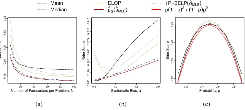
The results are summarized in two sets of figures: Figures 2.1a and 2.2a plot the Brier

scores (given by averaging over the systematic bias and the true probability) against the

number of forecasters per problem, Figures 2.1b and 2.2b plot the Brier score (given by

averaging over the number of forecasters per problem and the true probability) against the

systematic bias term, and Figures 2.1c and 2.2c plot the Brier scores (given by averaging

over the number of forecasters per problem and the systematic bias) against the true

proba-bility. Figure 2.1 presents the results underK = 30, and Figure 2.2 shows the results under

K = 100.

Given that pˆG(ˆaM LE) and 1P-BELP( ˆαM LE) performed better thanpˆG(ˆaBRI)and

1P-BELP( ˆαBRI), only the results associated with the maximum likelihood approach are

pre-sented. Comparing Figure 2.1 to Figure 2.2 shows that these two aggregators make very

good use of the training data and outperform the simple, parameterless aggregators as

the training set increases from K = 30 to K = 100 problems. Overall, our aggregator

ˆ

pG(ˆaM LE) achieves the lowest Brier score almost uniformly across Figures 2.2a to 2.2c.

This result, however, is more of a sanity-check than a surprising result as the data were

generated explicitly to match the model assumptions made bypˆG.

4_{This value was considered a realistic choice after analyzing the variance of the log-odds in our real-world}

(36)

Mean Median

ELOP p^_G(a^MLE)

1P−BELP(α^_MLE)

p(1−p)2+(1−p)p2

20 40 60 80 100

0.19

0.20

0.21

0.22

0.23

Number of Forecasters per Problem, N

Br

ier Score

(a)

0.5 1.0 1.5 2.0

0.185

0.190

0.195

0.200

0.205

0.210

0.215

Systematic Bias, a

Br

ier Score

(b)

0.2 0.4 0.6 0.8

0.10

0.15

0.20

0.25

Probability, p

Br

ier Score

(c)

Figure 2.1:K = 30synthetic problems for training. 1,000 problems for testing.

Mean Median

ELOP p^_G(a^MLE)

1P−BELP(α^_MLE)

p(1−p)2

+(1−p)p2

20 40 60 80 100

0.19

0.20

0.21

0.22

0.23

Number of Forecasters per Problem, N

Br

ier Score

(a)

0.5 1.0 1.5 2.0

0.185

0.190

0.195

0.200

0.205

0.210

0.215

Systematic Bias, a

Br

ier Score

(b)

0.2 0.4 0.6 0.8

0.10

0.15

0.20

0.25

Probability, p

Br

ier Score

(c)

Figure 2.2:K = 100synthetic problems for training. 1,000 problems for testing.

Based on Figures 2.1b and 2.2b, correcting for the bias when the data are actually

unbiased (a = 1.0) does not cause much harm. But correcting for the bias when the

data are truly biased (a 6= 1.0), yields noticeable performance benefits especially when

K = 100. Interestingly, the mean performs better than all other aggregators when the

(37)

are under-confident (a >1). To gain some understanding of this behavior, notice that in the

highly over-confident case the distribution of the forecasts tends to be very skewed in the

probability scale. The values in the long tail of such a distribution have a larger influence on

the mean than, say, the median of the probability forecasts. Given that the median is mostly

unaffected by these values, it produces an aggregate forecast that remains over-confident.

The mean, by contrast, is drawn towards 0.5 by the values in the long tail. This produces

an aggregate forecast that is less over-confident; hence improving forecast performance.

The improved performance, however, comes at a cost: when the true probability p is

very close to the extreme probabilities 0.0 and 1.0, the mean is, on average, the worst

performer among all the aggregators in the analysis. This difference in performance, which

is clear in Figures 2.1c and 2.2c, is more meaningful when compared to the baseline given

by p(1−p)2 _{+ (1}₋_p)p2_{. Given that the expected Brier score is minimized at the true}

probability, this line should be considered as the ultimate goal in Figures 2.1c and 2.2c.

Notice that all aggregators, except the mean, approach the linep(1−p)2+ (1−p)p2from

above aspgets closer to the extreme probabilities 0.0 and 1.0.

2.3.2 Synthetic Data: Misspecified Model

Next we evaluate the different aggregators on data that have not been generated from the

Logit-Normal distribution. The setup considered is an extension of the simulation study

introduced in Ranjan and Gneiting (2010) and further applied in Allard et al. (2012). Under

our extended version, the true probability for a problem withN forecasters is given by

p = Φ

N

X

i=1

ui

!

,

whereΦis the cumulative distribution function of a standard normal distribution, and each

ui

i.i.d.

(38)

process but only observesui. Then his calibrated estimate forpis given by

pi = Φ

ui

√

2N −1

Notice that the more forecasters are participating in a given problem, the less information

(proportionally) knowing ui gives the forecaster. Therefore as the number of forecasters

increases, the forecaster shrinks his estimate more and more towards 0.5. More specifically,

pi →Φ(0) = 0.5for alli= 1, . . . , N asN → ∞.

To give a real-world analogy of this setup, think of a group ofN people independently

voting on a binary event. Knowing everybody’s vote determines the final outcome. Given

that each person only knows his own vote, his proportional knowledge share diminishes

as more people enter the voting. As a result, his probability forecast for the final outcome

should shrink towards 0.5.

In our simulation, we varied the number of forecasters per problem, N, from 2 to 100

(with increments of one forecaster). Under each value ofN, the simulation ran for a total

of 10,000 iterations. Each iteration produced the true probabilities for theK problems and

their associated pools ofN probability estimates from the process described above. The

true probabilities were used to generate Bernoulli random variables that indicated which

events occurred and which did not. Testing was performed on a separate testing set

con-sisting of 1,000 problems, each with the same number of forecasters as the problems in the

training set. In the end, the resulting Brier scores were averaged to give an average Brier

score at each number of forecasters for each problem.

Figure 2.3 plots the average Brier score against the number of forecasters per problem

underK = 100problems. The same analysis was performed underK = 30. The results,

however, turned out to be almost identical to the results under K = 100 and hence, for

the sake of brevity, are not presented separately. Before discussing theK = 100 results,

(39)

Mean Median

ELOP p^_G(a^MLE)

1P−BELP(α^_MLE)

0 20 40 60 80 100

0.18

0.20

0.22

0.24

Number of Forecasters per Problem

Br

ier Score

Figure 2.3: 100 synthetic problems for training. 1,000 problems for testing.

many generally encountered data generating processes, having more data leads to increased

bias and is therefore harmful. As a result, we would expect the aggregators to perform

worse as the sample size increases. Based on Figure 2.3, the mean, median, and ELOP,

which do not aim to correct for the bias, in fact, degrade in terms of performance as the

number of forecasters increases. The one-parameter aggregators, pˆG and 1P-BELP, by

contrast, are able to stabilize the average Brier score despite the increasing bias in the

probability estimates. Overall, pˆG achieves the lowest Brier score across all numbers of

forecasters per problem.

2.3.3 Real Data: Predicting Geopolitical Events

We recruited over 1,300 forecasters, who ranged from graduate students to forecasting and

political science faculty and practitioners, and then asked them to give probability forecasts

(40)

centers, alumni associations, science bloggers, and word of mouth. Requirements included

at least a Bachelor’s degree and completion of psychological and political tests that took

roughly two hours. These measures assessed cognitive styles, cognitive abilities,

person-ality traits, political attitudes, and real-world knowledge. All forecasters knew that their

probability estimates would be assessed for accuracy using Brier scores. This incentivized

the forecasters to report their true beliefs instead of gaming the system. Forecasters

re-ceived $150 for meeting minimum participation requirements, regardless of their accuracy.

They also received status rewards for their performance via leaderboards displaying Brier

scores for the top 20 forecasters. Each of the 69 geopolitical events had two possible

out-comes. For instance, some of the questions were

Will the expansion of the European bailout fund be ratified by all 17 Eurozone

nations before 1 November 2011?

and

Will the Nikkei 225 index finish trading at or above 9,500 on 30 September

2011?

See the Appendix for a complete list of the 69 problems and associated summary statistics.

The forecasters were allowed to update their forecast as long as the question was active.

Some questions were active longer than others. The number of active days ranged from 2

to 173 days, with a mean of 54.7 days. It is important to note that this paper does not focus

on dynamic data. Instead we study pools of probability forecasts with no more than one

forecast given by a single expert. More specifically, we consider the first three days for

each problem because this is when the most of uncertainty is present. If an expert made

more than one forecast within these three days, we consider only his most recent forecast.

This results in 69 sets of probabilities with the number of forecasters per problem ranging

(41)

in every problem, we consider the experts completely anonymous (and interchangeable)

both within and across problems. Before we evaluate the results, however, we discuss

several practical matters that need to be taken into account when aggregating real-world

forecasting data.

2.3.3.1 Extreme Values and Inconsistent Data

For any value ofa, the aggregatorpˆGsatisfies the0/1forcing property which states that if

the pool of forecasts includes an extreme value, that is either zero or one but not both, then

the estimator should return that extreme value (see, e.g., Allard et al. (2012)). This property

is desirable if one of the forecasters happens to know the final outcome of the event with

absolute confidence. Unfortunately, experts can make such absolute claims even when they

are not completely sure of the outcome. For instance, each of the forecast pools associated

with the 69 questions in our data contained both a zero and a one. In any such dataset, an

aggregator that is based on the geometric mean of the odds is undefined.

These data inconsistencies can be avoided by adding and subtracting a small quantity

from zeros and ones, respectively. Ariely et al. (2000) suggest changing p = 0 and 1to

p = 0.02and0.98, respectively. Allard et al. (2012) only consider probabilities that fall

within a constrained interval, say [0.001,0.999], and throw out the rest. Given that this

implies ignoring a portion of the data, we take an approach similar to that of Ariely et al.

(2000) and replace p = 0 and 1 with p = 0.01 and 0.99, respectively. In the case of

multinomial events, the modified probabilities should be normalized to sum to one. This

forces the probability estimates to the open interval(0,1). The transformation will shift the

truncated values even closer to their true extreme values. For instance, ifa is larger than

two, which often is the case, 0.01 and 0.99 would be transformed at least to 0.0001 and

0.9999, respectively.

(42)

given by the arithmetic mean of the probabilities. This gives us the following estimator

ˆ

pA(a) =

h

¯

p

1−p¯

ia

1 +h₁₋p¯_p_¯ia ,

wherep¯= _N1 PN

i=1pi. The subindex emphasizes the use of the arithmetic mean. The two

estimators pˆG and pˆA will differ the most when the set of probability forecasts includes

values close to the extremes. Therefore the larger the variance termσ2 of the Logit-Normal

model is the more we would expect these two estimators to differ. For comparison’s sake,

we have includedpˆAin the real-world data analysis.

A similar problem arises with the logarithmic opinion pool, where zero predictions

from experts can be viewed as “vetoes” (see Genest and Zidek (1986)). To address this, we

replacedp= 0withp= 0.01and normalized the probabilities to sum to one.

2.3.3.2 Aggregator Comparison on Expert Data

This section evaluates the aggregators on the first three days of the 69 problems in our

dataset. The evaluation begins by exploring the impact of number of forecasters per

prob-lem on predictive power. Each run of the simulation fixes the number of forecasters per

problem and samples a random subset (of this size) of forecasters within each problem.

These subsets are then used for training and computing a Brier score. The sampling

pro-cedure is repeated 1,000 times during the simulation. The resulting 1,000 Brier scores are

averaged to obtain an overall performance measure under the given number of forecasters

per problem.

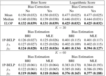
Figure 2.4 plots the average Brier score against the number of forecasters per problem.

The MLE aggregatorpˆG achieves the lowest Brier score across all numbers of forecasters

per problem. The two aggregatorspˆAand P1-BELP perform so similarly that their average

(43)

Mean Median ELOP

p^A(a^BRI)

p^_A(a^MLE)

p^_G(a^BRI)

p ^

G(a^MLE)

1P−BELP(α^_BRI)

1P−BELP(α^MLE)

20 40 60 80

0.12

0.13

0.14

0.15

0.16

Number of Forecasters per Problem

Br

ier Score

Figure 2.4: 69 real-world problems for training. The first three days; much uncertainty.

ˆ

pAappears to widen as the number of forecasters increases.

It merits note that most of the improvement across the different approaches occurs

before roughly 50 forecasters per problem. This suggests a new strategy for collecting data:

instead of having a large number of forecasters making predictions on a few problems, we

should have around 50 forecasters involved with a large number of problems. With a larger

number of problems, a more accurate estimate of the systematic bias could be acquired,

possibly leading to improved forecast performance.

A similar analysis was performed with the last three days of each problem. The average

Brier scores, however, were very close to zero. There was, in fact, so much certainty among

the forecasters, that simply taking the median gave an aggregate forecast very close to the

truth. For this reason, we decided to not present these results in this paper.

The average Brier scores in Figure 2.4 are based on the training error. No separate

(44)

in a large enough sample does not overfit significantly. Figure 2.5 plots the Brier score for

ˆ

pG under varying levels ofa. Given that the optimal level of a is around 2.0, the experts

(as a group) appear under confident, and pˆG gains its advantage by shifting each of the

probability forecasts closer to its nearest boundary point (0.0 or 1.0).

Running arepeated sub-sampling validationwith a training set of sizeK and a testing

set of size69−Ksupports the results shown in Figure 2.4. Table 2.1 shows the results after

runningrepeated sub-sampling validationwithK = 30andK = 60a total of 1,000 times

and then averaging the resulting 1,000 (testing) Brier scores. For the sake of consistency,

we have also included the average logarithmic scores:

− 1

69−K

X

k=1

Zklog(ˆpk) + (1−Zk) log(1−pˆk)

wherepˆjis the probability estimate andZj is the event indicator for thejth testing problem

defined earlier in Section 2.2.2. The values given in parentheses are the estimated standard

deviations of the testing scores. Given that the mean, median, and ELOP do not use training

data, their reported scores are based on the simulation withK = 30that uses a larger testing

set.

In Table 2.1 we have also included the bias-corrected versions of the mean, median,

and ELOP. This correction was attained by applying bootstrap sampling to the pool of

probabilities for a total of 1,000 times. More specifically,

ˆ

pf,k = 2f(pk)−

1 1000

1000

X

i=1

fp(_k,bsi) ,

(45)

Brier Score Logarithmic Score

Bias Correction Bias Correction

No Yes No Yes

Mean 0.150 (0.032) 0.150 (0.032) 0.477 (0.025) 0.477 (0.025)

Median 0.140 (0.038) 0.139 (0.038) 0.446 (0.031) 0.444 (0.031)

ELOP 0.132 (0.039) 0.131 (0.039) 0.425 (0.032) 0.425 (0.032)

K = 30

Bias Estimation Bias Estimation

BRI MLE BRI MLE

1P-BELP 0.126 (0.027) 0.125 (0.026) 0.401 (0.115) 0.401 (0.117)

ˆ

pA 0.127 (0.027) 0.125 (0.026) 0.402 (0.109) 0.402 (0.115)

ˆ

pG 0.124 (0.028) 0.122 (0.026) 0.401 (0.134) 0.394 (0.127)

K = 60

Bias Estimation Bias Estimation

BRI MLE BRI MLE

1P-BELP 0.122 (0.061) 0.121 (0.064) 0.383 (0.170) 0.384 (0.193)

ˆ

pA 0.122 (0.061) 0.121 (0.065) 0.385 (0.168) 0.386 (0.190)

ˆ

pG 0.119 (0.060) 0.118 (0.064) 0.376 (0.165) 0.377 (0.188)

Table 2.1: K problems for training. 69−K problems for testing. 1,000 repetitions. The

values in the parentheses are the estimated standard deviations of the testing scores.

improved the performance only by a small margin if at all.

For convenience, we have bolded the lowest scores in each column of the three boxes.

Overall, the ranking of the aggregators on relative performances is the same as in Figure

2.4. As seen before, pˆG(ˆaM LE) achieves the lowest Brier and logarithmic scores by a

noticeable margin.

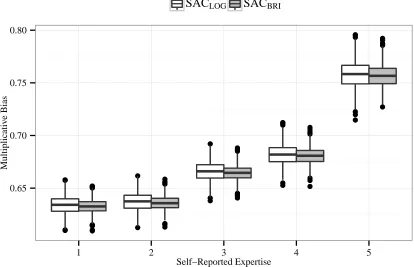
2.3.3.3 Less Transformation for More Expertise

Earlier we proposed that the more expertise the forecaster has, the less systematic bias can

be found in his probability forecasts. This means that his forecasts require less

transfor-mation, i.e. a lower level of a. To evaluate this interpretation, we asked forecasters to

self-assess their level of expertise on the topic. The level of expertise was measured on a

Partial Information Framework: Basic Theory and Applications

University of Pennsylvania

ScholarlyCommons

Partial Information Framework: Basic Theory and

Applications

Ville Antton Satopää

Partial Information Framework: Basic Theory and Applications

PARTIAL INFORMATION

FRAMEWORK: BASIC THEORY AND

APPLICATIONS

Ville A. Satop¨a¨a

A DISSERTATION

Statistics

For the Graduate Group in

Managerial Science and Applied Economics

Presented to the Faculties of the University of Pennsylvania

Partial Fulfillment of the Requirements for the

Degree of Doctor of Philosophy

2016

Dedication

Acknowledgments

ABSTRACT

PARTIAL INFORMATION FRAMEWORK:

BASIC THEORY AND APPLICATIONS

Ville A. Satop¨a¨a

Shane T. Jensen

Lyle H. Ungar

Contents

List of Tables

List of Figures

1

Introduction

2

Combining Multiple Probability Predictions Using

a Simple Logit Model

Abstract

2.1

Introduction

2.2

Theory

2.2.1

Model-based Aggregator

2.2.2

Estimating Systematic Bias

2.2.3

Extensions to the Aggregator

2.3

Results and Discussion

2.3.1

Synthetic Data: Correctly Specified Model

2.3.2

Synthetic Data: Misspecified Model

2.3.3

Real Data: Predicting Geopolitical Events