PERFORMANCE ANALYSIS OF IMAGE
DENOISING IN LIFTING WAVELET
TRANSFORM
G.M.Rajathi, Asst.professor,Dept of ECE Sri Ramakrishna Engineering college,
Tamil Nadu, Coimbatore, [email protected]
Dr.R. Rangarajan ,
Principal
Indus College of Engineering, Coimbatore
Abstract-Images are contaminated by noise due to several unavoidable reasons, Poor image sensors, imperfect instruments, problems with data acquisition process, transmission errors and interfering natural phenomena are its main sources. Therefore, it is necessary to detect and remove noises present in the images. Reserving the details of an image and removing the random noise as far as possible is the goal of image denoising approaches . Lifting wavelet transform (LWT)is based on the theory of lazy wavelet and completely recoverable filter banks, improving the wavelet and its performance through the lifting process under the condition of maintaining the feature of the wavelet compared with the classical constructions (DWT) is rely on the Fourier transform. In this paper we compare the image denoising performance of LWT with DWT . We demonstrated through
simulations with images contaminated by white Gaussian noise that exhibits performance in both PSNR (Peak Signal-to-Noise Ratio) and visual effect.
Keywords: Image Denoising, LWT,DWT, PSNR
1.INTRODUCTION
The denoising of a natural image corrupted by Gaussian noise is a classic problem in signal processing .The wavelet transform has become an important tool for this problem due to its energy compaction property .Indeed, wavelets[6][8] provide a framework for signal decomposition in the form of a sequence of signals known as approximation signals with decreasing resolution supplemented by a sequence of additional touches called details . Denoising or estimation of functions, involves reconstituting the signal as well as possible on the basis of the observations of a useful signal corrupted by noise The methods based on wavelet representations yield very simple algorithms that are often more powerful and easy to work with than traditional methods of function estimation. It consists of decomposing the observed signal into wavelets and using thresholds to select the coefficients, from which a signal is synthesized . Image denoising algorithm consists of few steps, consider an input signal X(t) and noise signal n(t ). Add these components to get noisy data y (t ) i.e. X(t )+n (t )=y (T ) Here the noise is Gaussian, then apply wavelet transform to get W(t ). Modify the wavelet coefficient W(t ) using different threshold algorithm and take inverse wavelet transform to get denoising image X( t).
2.Lifting wavelet transform
The Wavelet Transform provides a time-frequency representation of the signal. It was developed to overcome the short coming of the Short Time Fourier Transform (STFT), the Wavelet Transform uses multi-resolution technique by which different frequencies are analyzed with different resolutions. Advantage of wavelet analysis is the ability to perform local analysis. Wavelet analysis is capable of revealing aspects of data that other signal analysis techniques miss aspects like trends, breakdown points, discontinuities in higher derivatives, and self-similarity. Furthermore, because it affords a different view of data than those presented by traditional techniques, wavelet analysis can often compress or de-noise a signal without appreciable degradation. Wavelet analysis can be applied to two-dimensional data (images) and, in principle, to higher dimensional data.
is a technique for both designing wavelets and performing the discrete wavelet transform. The lifting allows one to custom design the filters needed in the transform algorithm. Compared with the first-generation wavelet, the lifting scheme could complete the wavelet transform currently without allocating additional memory, so it is easy to achieve with chips; the algorithm is simple and suitable for parallel processing, which makes the computation more fast; it could realize integral wavelet transform, which has wide potential applications
2.1Basic principles of lifting scheme
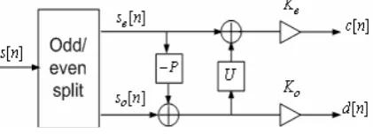
The second generation of wavelets,[1]which is under the name of lifting scheme, was introduced by Swelden. Lifting wavelet transform is also known as integral wavelet transform. The lifting algorithm can be computed in three main phases, namely:
1.Split Phase 2.Predict Phase 3.Update Phase
Signal is s[n] , then it is transformed into approximation signal c[n] and detail signal d[n]through wavelet. This is illustrated in the figure1 as
Fig. 1. Signal Decomposition in lifting Scheme
Split
Split the original signal s[n]into two non overlapping parts which are two subsets se[n] and so[n] split in even and odd orders generally, where
Predict
If the original signal s[n]possesses local correlation, then se[n]and so[n]also have local correlation, therefore , one subset may be used to predict the other subset,
and an odd sequence is generally predicted through an even sequence, that is
In the equation, P is a prediction operator, which reflects the correlation degree between data. P(se)[n]
expresses that predict the value of d[n]by some combination of the value of se[n]. Update
c[n] in the above figure is the approximation signal obtained after decomposition, and one important property of c[n] is that its mean value shall be equal to the mean value of the original signal s[n]. Therefore, even sequence number subset se[n] can be updated by detail subset d[n], which is shown as follows when expressed by c[n]
In the above equation, operator U represents some combination of d[n]. In a similar way, in case the decompositions shown in the above two steps are conducted on the approximation signal c[n] obtained after decomposition again, then a multistage decomposition of the original signal can be obtained.
2.2 INVERSE LIFTING WAVELET TRANSFORM
The operation is working backwards from the forward lifting operation. The averages (even elements) become the input for the next recursive step of the forward transform. The number of data elements processed by the wavelet transform must be a power of two. If there are 2n data elements, the first step of the forward transform will produce 2n-1 averages and 2n-1 differences (between the prediction and the actual odd element value). These differences are sometimes referred to as wavelet coefficients.
Fig2 :Inverse lifting wavelet transform
In the inverse step,the upate step is followed by predict step and finally the odd and even components are merged which interleaves the odd and even elements back into one data stream.The equation for the inverse lifting steps are given by:
2.3COMPARISION BETWEEN FILTER BASED DWT AND LIFTING SCHEME
The lifting scheme is a new method for constructing biorthogonal wavelets[4][7]. The main difference with classical constructions is that it does not rely on the Fourier transform. The lifting scheme and filter based DWT can be compared as follows:
The lifting scheme allows a faster implementation of the wavelet transform. Traditionally, the fast wavelet transform is calculated with a two-band sub band transform scheme. In each step the signal is split into a high pass and low pass band and then sub sampled. Recursion occurs on the low pass band. The lifting scheme makes optimal use of similarities between the high and low pass filters to speed up the calculation. The number of hops can be reduced by a factor of two.
The lifting scheme allows a fully in-place calculation of the wavelet transform. In other Words , no auxiliary memory is needed and the original signal (image) can be replaced with its wavelet transform.
In the classical case, it is not immediately clear that the inverse wavelet transform actually is the inverse of the forward transform because here the filter is used to obtain DWT. Only with the Fourier transform one can convince oneself of the perfect reconstruction property. With the lifting scheme, the inverse wavelet transform can immediately be found by undoing the operations of the forward transform..The transform coefficients from LWT are integers, overcoming the weakness of quantizing errors from the traditional wavelet transform 2.3 LIFTING BACKGROUND
The DWT is defined by four filters Algorithm[7]. ,the perfect reconstruction property, the two conditions for perfect reconstruction are
Hs(z) Ha(z–1) + Gs(z) Ga(z–1) = 2 z–d Hs(z) Ha(–z–1) + Gs(z) Ga(–z–1) = 0
where Hs(z), Gs(z) are the z-transforms of the filters hs, gs respectively, and Ha(–z–1) and Ga(–z–1) are the z-transforms of ha, ga respectively.The first condition is usually (incorrectly) called the perfect reconstruction condition and the second is the anti-aliasing condition.The four filters (or equivalently four z-transforms) verifying the (PR) conditions as biorthogonal quadruplets.
The principle of lifting is to generate from a given biorthogonal quadruplet a new one by applying a finite sequence of primal or dual elementary lifting steps (ELS).A primal ELS generates from the biorthogonal quadruplet (Ha,Ga,Hs,Gs), a new one (HaN,Ga,Hs,GsN) by
HaN (z) = Ha(z) – Ga(z) S(z–2) GsN (z) = Gs(z) + Hs(z) S(z2)
where S is any Laurent polynomial.
involving positive and negative integer powers of z. The degree of C is defined as (pmax–pmin).Similarly, a dual ELS generates from the same initial biorthogonal quadruplet, a new one (Ha,GaN,HsH,Gs) by
HsN (z) = Hs(z) + Gs(z) T(z2) GaN (z) = Ga(z) – Ha(z) T(z–2)
where T is any Laurent polynomial.These new quadruplets verify the perfect reconstruction conditions (PR). Note that even if the initial biorthogonal quadruplet is associated with "true" wavelets, the new ones are not automatically associated with "true" wavelets but remain useful for discrete wavelet transform of sequences instead of functions.
The previous results are sufficient to generate lifted quadruplets. Nevertheless, by introducing the polyphase matrix, interesting theoretical and algorithmic results can be derived. The synthesis polyphase matrix P associated with the biorthogonal quadruplet (Ha,Ga,Hs,Gs) is the 2-by-2 matrix defined (using the MATLAB conventions) by
P(z)=[even(Hs)(z) ven(Gs)(z) ; odd(Hs)(z) odd(Gs)(z) ] Where
even(C)(z2) = (C(z) + C(–z)) / 2 odd(C)(z2) = (C(z) – C(–z)) / 2z–1
Then after a primal lifting the new polyphase matrix PN is obtained simply from P the initial one by PN(z) = P(z) * [1 S(z) ; 0 1]
P itself can be decomposed, up to a normalization, as a product of matrices of the form [1 S(z) ; 0 1] or [1 0 ; T(z) 1] as soon as P is associated with a biorthogonal quadruplet. This form leads to the efficient polyphase algorithm. Another useful consequence is that any biorthogonal quadruplet can be obtained by a sequence of ELS, up to a normalization, starting from a particular seed called the "lazy" wavelet (which is not a "true" wavelet and which simply separates odd and even samples of the filter bank input signal).
So, in the Wavelet Toolbox software, the key structure to perform what we commonly call the lifting wavelet transform (LWT) is a lifting scheme, which is simply a sequence of ELS and normalization steps.
3. Algorithm for Denoising
Denoising [8] can be achieved by applying a thresholding operator to the wavelet coefficient followed by reconstruction of the signal to the original image domain.
Thresholding operators Hard thresholding D(U, λ)=U for all |U|> λ
=0 otherwise Soft thresholding
D(U, λ) = sign(U)(U- λ) for all U> λ = 0 otherwise Semisoft thresholding
It is a family of non-linearities that interpolates between hard and soft thresholding. D(U, λ)=0 |U|<= λ1
=sign(U) λ2(|U|- λ1) λ1<=|U|<= λ2 λ2- λ1
=U |U|> λ2 Where threshold λ= σ√2logn
The parameter noise variance σ is estimated by
σ^2={( median|Yi|)/0.6745 Yi each subband (1) where 0.6745 is the experiential value [9].
Steps involved in denoising
1. Decompose the image into subbands
2. Estimate the noise variance in the noisy image using above equation 1 4. For each subband
(a) Compute the threshold λ
(b) Apply thresholding to the subbands
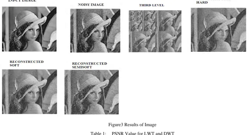
Figure3 Results of Image
Table 1: PSNR Value for LWT and DWT
4. Conclusion
In this paper ,we compare Performance of denoising using classical filter based DWT and LWT. Performance of denoising algorithms is measured using quantitative performance measures such as peak signal-to-noise ratio(PSNR), as well as in terms of visual quality of the images. A semisoft thresholding process show a better enhancement than hard and soft threshold method to denoise the image. With careful tuning of threshold parameter for a image, we can achieve best denoising effect within thresholding frame work semisoft thresholding. Comparisons indicates that the denoising method using LWT can get a better performance with lazy wavelet filter
REFERENCES
[1] Sweldens W_The lifting scheme_a construction of second generation wavelets [J]_SIAM J_Math_Ana1_1997. 29(2)_ 5l546. [2] Yang Fusheng. Engineering Analysis and Application of Wavelet Transform [M]. Beijing: Science Press, 2001.
[3] Sweldens W 1995 The lifting scheme: A new philosophy in biorthogonal wavelet constructions: Proc. SPIE-Int. Soc. Opt. Eng. 256968-79
[4] Sweldens W 1996 The lifting scheme: A custom-design construction of biorthogonal wavelets: J. Appl. Comput. Harmon. Anal 3 186-200
[5] R.L. Claypoole, RG. Baraniuk, R.D. Nowak "Lifting Construction of Non-Linear Wavelet Transforms", IEEE -SP Symposium on Time-Frequency and Time-Scale Analysis TFTS-98, pp.49-52, Pittsburgh 1998.
[6] R.L. Claypoole, RG. Baraniuk, R.D. Nowak "Adaptive Wavelet Transforms via Lifting," IEEE Conf. on Acoustics, Speech and Signal Processing, Phoenix, 1999.
[7] A book on “Image processing MATLAB toolbox”. [8] D. L. Donoho, (1995) “De-noising by Soft Thresholding,”
IEEE Trans. on Inform, Theory, 41, No. 3, pp. 613- 627Javier Portilla, Vasily Strela, Martin J.
[9] I.M. Johnstone, B.W. Silverman, “Wavelet ThresholdEstimators for Data with Correlated Noise”, Journalof Royal Statistical Soc., vol.B59, pp.319~351, 1997.
[10] E. Zhang, S. Huang, “A New Image DenoisingMethod based on the Dependency Wavelet Coefficients”,Proceedings of the 3rd InternationalConference on Machine Learning and Cybermetics,Shanghai, Aug., 2004
N
Nooiissee v
vaarriiaanncce e
H
HAARRD SOFT D SEMI -SOFT
L
LWWTT DDWWTT LLWWTT DDWWTT LLWWTT DWT
4
40 0 2244..665 23.12 5 2244..774 23.29 4 2244..9922 23.69
5
50 0 2244..338 21.53 8 2244..444 21.82 4 2244..7733 21.92
6
60 0 2244..008 20.01 8 2244..115 20.31 5 2244..6600 20.74
7