University of Pennsylvania
ScholarlyCommons
Publicly Accessible Penn Dissertations
1-1-2016
Essays on Labor and Risk
Patrick E. Dejarnette
University of Pennsylvania, [email protected]
Follow this and additional works at:
http://repository.upenn.edu/edissertations
Part of the
Economic Theory Commons
, and the
Labor Economics Commons
This paper is posted at ScholarlyCommons.http://repository.upenn.edu/edissertations/1679 For more information, please [email protected].
Recommended Citation
Essays on Labor and Risk
Abstract
This dissertation presents three essays in labor economics and risk. Chapter 1 examines how past effort can impact current effort, such as when effort is reduced following an interruption. I present a series of real-effort incentivized experiments in which both piece rates and leisure options were manipulated and find effort displays significant stickiness, even in the absence of switching costs. I demonstrate that this intertemporal evidence is indicative of effort “momentum”, rather than on-the-job learning, reciprocity, or income targeting. When employing an instrumental variables (IV) approach, approximately 50\% of the effort increase persists for 5 minutes after incentives return to baseline. Thus if a worker suffers a complete interruption in
productivity, it would take an average of 15 minutes to return to 90\% of prior work effort. I further demonstrate that advanced knowledge does not significantly reduce this productivity loss.
Chapter 2 examines how risk preferences differ over goods and in-kind monetary rewards. I study an
incentivized experiment in which subjects allocate bundles of either Amazon.com goods or Amazon.com gift credit (which must be spent immediately) across uncertain states. Under a standard model of perfect
information of prices and goods available, I demonstrate risk preferences across these treatments would be identical. In practice, I uncover substantial differences in risk preferences across goods and in-kind monetary rewards. With additional treatments, I find no evidence that these differences are driven by price or product uncertainty.
Chapter 3 is joint work with David Dillenberger, Daniel Gottlieb, and Pietro Ortoleva. We study preferences over lotteries that pay a specific prize at uncertain dates. Expected Utility with convex discounting implies that individuals prefer receiving x in a random date with mean t over receiving x in t days for sure. Our experiment rejects this prediction. It suggests a link between preferences for payments at certain dates and standard risk aversion. Epstein-Zin (1989) preferences accommodate such behavior, and fit the data better than a model with probability weighting.
Degree Type Dissertation
Degree Name
Doctor of Philosophy (PhD)
Graduate Group Applied Economics
First Advisor Jeremy Tobacman
Keywords
Subject Categories
ESSAYS ON LABOR AND RISK
Patrick E. DeJarnette
A DISSERTATION
in
Applied Economics
For the Graduate Group in Managerial Science and Applied Economics
Presented to the Faculties of the University of Pennsylvania
in
Partial Fulfillment of the Requirements for the
Degree of Doctor of Philosophy
2016
Supervisor of Dissertation
_____________________
Jeremy Tobacman
Assistant Professor of Business Economics and Public Policy
Graduate Group Chairperson
______________________
Eric Bradlow, K.P. Chao Professor; Professor of Marketing, Statistics, and Education
Dissertation Committee:
Iwan Barankay, Associate Professor of Business Economics and Public Policy
ESSAYS ON LABOR AND RISK
c COPYRIGHT
2016
Patrick Edward DeJarnette
This work is licensed under the
Creative Commons Attribution
NonCommercial-ShareAlike 3.0
License
To view a copy of this license, visit
To my family,
ACKNOWLEDGEMENT
This dissertation would not have been possible without the support, guidance, and
encour-agement of many people. First and foremost, my tireless dissertation committee, Jeremy
Tobacman, Iwan Barankay, Daniel Gottlieb, Robert Jensen, and Judd Kessler. Jeremy’s
persistence and patience, Iwan’s advice, Daniel’s encouragement, Rob’s guiding hand, and
Judd’s insight have all played a crucial role in getting me to where I am today. I am
especially thankful to my primary advisor Jeremy who has met with me weekly for over
4 years and has weathered both the ups and downs of the research process. Without his
extraordinary e↵orts, I would not have weathered this storm.
I am indebted to the many readers who gave me feedback on my dissertation at various
stages. Including comments from Paul Bruton, Mark Clements, Amanda Chuan, Ulrich
Do-raszelski, Clayton Featherstone, Fernando Ferreira, Joseph Harrington, Sonia Ja↵e, Corinne
Low, Anita Mukherjee, Todd Sinai, Charles Sprenger, Shing-Yi Wang, Kate Wilhelm, and
Tomoyoshi Yabu. I am also grateful to my excellent co-authors, David Dillenberger, Daniel
Gottlieb, and Pietro Ortoleva, without whom Chapter 3 would not have been possible. This
research (specifically Chapter 1 and 2) was also supported by a grant from the Wharton
School’s Mack Institute for Innovation Management.
More than anyone though, Tian Cai had the largest impact on my experience in graduate
school. To her I owe my deepest gratitude for supporting me and serving as my guiding star.
Her incredible love and remarkable insight can be found on every page of this dissertation.
I thank her for inspiring me and for always being my better half.
Finally, I owe everything to the rest of my family, particularly my mother Mary Pat, my
father Edward, my brother Robert, and my sister Stephanie. Without all of them, I would
never have reached where I am today. Their support and insistence have made me the
ABSTRACT
ESSAYS ON LABOR AND RISK
Patrick E. DeJarnette
Jeremy Tobacman
This dissertation presents three essays in labor economics and risk. Chapter 1 examines how
past e↵ort can impact current e↵ort, such as when e↵ort is reduced following an interruption.
I present a series of real-e↵ort incentivized experiments in which both piece rates and
leisure options were manipulated and find e↵ort displays significant stickiness, even in the
absence of switching costs. I demonstrate that this intertemporal evidence is indicative of
e↵ort momentum, rather than on-the-job learning, reciprocity, or income targeting. When
employing an instrumental variables (IV) approach, approximately 50% of the e↵ort increase
persists for 5 minutes after incentives return to baseline. Thus if a worker su↵ers a complete
interruption in productivity, it would take an average of 15 minutes to return to 90% of
prior work e↵ort. I further demonstrate that advanced knowledge does not significantly
reduce this productivity loss.
Chapter 2 examines how risk preferences di↵er over goods and in-kind monetary rewards. I
study an incentivized experiment in which subjects allocate bundles of either Amazon.com
goods or Amazon.com gift credit (which must be spent immediately) across uncertain states.
Under a standard model of perfect information of prices and goods available, I demonstrate
risk preferences across these treatments would be identical. In practice, I uncover
sub-stantial di↵erences in risk preferences across goods and in-kind monetary rewards. With
additional treatments, I find no evidence that these di↵erences are driven by price or product
uncertainty.
We study preferences over lotteries that pay a specific prize at uncertain dates. Expected
Utility with convex discounting implies that individuals prefer receiving x in a random date
with mean t over receiving x in t days for sure. Our experiment rejects this prediction. It
suggests a link between preferences for payments at certain dates and standard risk aversion.
Epstein-Zin (1989) preferences accommodate such behavior, and fit the data better than a
TABLE OF CONTENTS
ACKNOWLEDGEMENT . . . iv
ABSTRACT . . . v
LIST OF TABLES . . . x
LIST OF ILLUSTRATIONS . . . xi
CHAPTER 1 : E↵ort Momentum . . . 1
1.1 Introduction . . . 1
1.2 Predictions . . . 10
1.3 Experiment Design Overview . . . 19
1.4 Empirical Specifications . . . 24
1.5 Experiment Results . . . 26
1.6 Alternative Theories . . . 33
1.7 Conclusion . . . 35
1.8 Figures . . . 38
1.9 Tables . . . 43
CHAPTER 2 : Risk Over Goods . . . 56
2.1 Introduction . . . 56
2.2 Theory . . . 58
2.3 Experiment Design Overview . . . 63
2.4 Experiment Results . . . 65
2.5 Conclusion . . . 68
2.6 Figures . . . 71
CHAPTER 3 : Time Lotteries . . . 81
3.1 Introduction . . . 81
3.2 DEU and Attitudes towards Time Lotteries . . . 87
3.3 Beyond DEU: Epstein Zin Preferences and Probability Weighting . . . 91
3.4 Experiment . . . 98
APPENDIX . . . 110
LIST OF TABLES
TABLE 1 : Predictions Summary Table . . . 19
TABLE 2 : Design Summary Table . . . 22
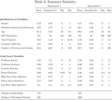
TABLE 3 : Summary Statistics . . . 43
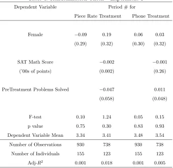
TABLE 4 : Randomization Check – Experiment 1 . . . 44
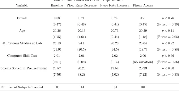
TABLE 5 : Randomization Check – Experiment 2 . . . 45
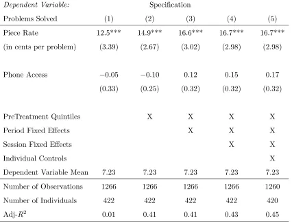
TABLE 6 : Contemporaneous Piece Rate and Phone Access: Impact on E↵ort – Experiment 1 . . . 46
TABLE 7 : Contemporaneous Piece Rate and Phone Access: Impact on E↵ort – Experiment 2 . . . 47
TABLE 8 : Previous Period Piece Rate and Phone Access: Impact on E↵ort – Experiment 1 . . . 48
TABLE 9 : Previous Period Piece Rate and Phone Access: Impact on E↵ort – Experiment 2 . . . 49
TABLE 10 : Phone Access by Gender: Impact on E↵ort – Experiment 2 . . . . 50
TABLE 11 : Phone Access by Gender: Impact on E↵ort – Experiment 2 . . . . 51
TABLE 12 : Next Period Piece Rate and Phone Access: Impact on E↵ort – Ex-periment 1 . . . 52
TABLE 13 : Next Period Piece Rate and Phone Access: Impact on E↵ort – Ex-periment 2 . . . 53
TABLE 14 : Previous E↵ort Instrumental Variable: Impact on E↵ort – Experi-ment 2 . . . 54
TABLE 15 : Period or Total Earnings Salience: Impact on Earnings – Experiment 2 55 TABLE 16 : Summary Statistics . . . 74
TABLE 18 : Credit and $100: Impact on Standard Deviation of Selection Value 76
TABLE 19 : Credit and $100: Impact on Standard Deviation of Selection Value
(Normalized) . . . 77
TABLE 20 : Credit and $100: Impact on Equality of Selection Values . . . 78
TABLE 21 : OLS Impact of Search on Standard Deviation of Selection Value . . 79
TABLE 22 : IV Impact of Search on Standard Deviation of Selection Value . . . 80
TABLE 23 : Questions in Part I . . . 100
TABLE 24 : Questions in Part II . . . 101
TABLE 25 : Questions in Part III . . . 101
TABLE 26 : Percentage of RATL in each question . . . 104
TABLE 27 : Frequency of RATL answers in Part I . . . 104
TABLE 28 : Proportion of RATL subjects . . . 106
TABLE 29 : Probit Regressions: RATL and Convexity and Certainty Bias . . . 108
TABLE 30 : Probit Regressions: RATL and Atemporal Risk Aversion . . . 108
TABLE 31 : Proportion of RATL subjects . . . 146
TABLE 32 : Probit Regressions: RATL and Atemporal Risk Aversion . . . 146
LIST OF ILLUSTRATIONS
FIGURE 1 : Example of Counting Problem Task . . . 38
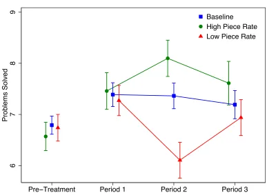
FIGURE 2 : Solved Problems by Period – Experiment 2 . . . 39
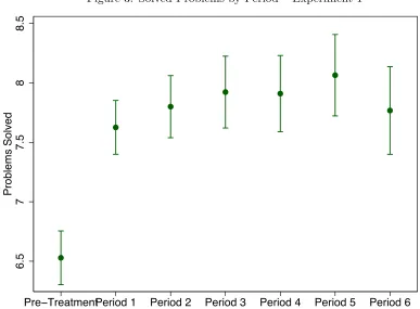
FIGURE 3 : Solved Problems by Period – Experiment 1 . . . 40
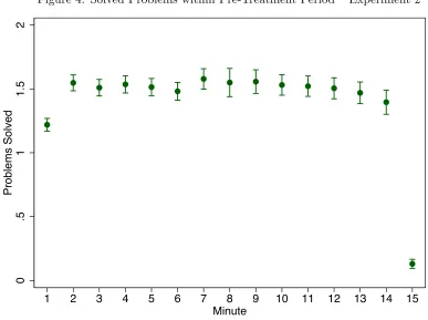
FIGURE 4 : Solved Problems within Pre-Treatment Period – Experiment 2 . . 41
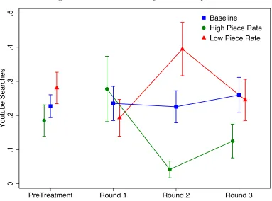
FIGURE 5 : YouTube Searches by Period – Experiment 2 . . . 42
FIGURE 6 : Example of Good Selection . . . 71
FIGURE 7 : Distribution of the Smaller Value When Total is $20 . . . 72
FIGURE 8 : Distribution of the Smaller Value (Normalized) When Total is $20 73
FIGURE 9 : Temporal discount functions . . . 82
FIGURE 10 : Discount functions are convex . . . 90
CHAPTER 1 : E↵ort Momentum
1.1. Introduction
By some estimates, interruptions disrupt 1.5 to 2.1 hours per work day for over 56 million
US “knowledge workers” (Gonzalez and Mark (2004); Spira and Feintuch (2005)).
Obser-vational studies show that hospital workers are interrupted 5 times per hour (Weigl et al.
(2014); Berg et al. (2013)) while software developers and managers are interrupted 25 times
per day (Gonzalez and Mark (2004)).1 In similar studies, 15-23% of interrupted work is
not resumed on the same day, a particular concern within the health services literature
(Westbrook et al. (2010); Mark et al. (2005)). However, this evidence is difficult to
inter-pret when the interruptions themselves may be necessary, as within a hospital’s emergency
department. In other contexts, interruptions from a manager may reduce principal-agent
concerns through increased monitoring or communication as formulated by Coviello et al.
(2014). Interruptions from a co-worker could increase a firm’s total output, even at the
expense of the interrupted worker. As a result, it might be presumptuous to target
inter-ruptions themselves as a source of productivity waste.
At the heart of the question of how interruptions a↵ect behavior is whether there is stickiness
in e↵ort allocation. If so, interruptions could undermine productivity due to unplanned
e↵ort reduction following an interruption. This paper answers this more general question
of whether productivity loss persists over time, and if so, what might be done to recover it.
This “loss of momentum” is often posited by the psychology literature,2 media,3 and con-sulting reports,4 but has not been thoroughly examined within the economics literature. 1While half of these are considered “internal” interruptions, which may be more indicative of task jug-gling (Coviello et al. (2014)), the remaining half of “external” interruptions are arguably the most time intensive. For example, the data in Gonzalez and Mark (2004) also shows that 1.5 hours per day are spent on unscheduled meetings such as workers stopping by or talking through cubicle walls.
2See an extensive psychology literature on “flow”, cf. Nakamura and Csikszentmihalyi (2002); Scha↵er (2013), in which clear tasks with adequate challenge and objective goals enables a continuous work state.
3E.g. “First, there is the diversion itself, taking your employees o↵ task after they have assembled the
resources and thinking necessary for that particular task. Then there is the restart—reassembling the re-sources, thoughts, and readiness. There is the loss of momentum caused by the initial distraction from the original purpose.” (Brown (2015))
The closest literature on intertemporal labor supply tends to focus on longer time scales
and hours worked rather than output (Camerer et al. (1997); Oettinger (1999); Farber (2005,
2008); Crawford and Meng (2011); Chetty et al. (2011)). Within this literature, Fehr and
Goette (2007) employ a field experiment on bicycle riders and finds evidence consistent with
a model in which past e↵ort exhausts riders, making additional e↵ort more costly. Under
this model, an exogenous interruption in e↵ort could actually boost future productivity as
the worker has had a chance to “catch their breath”.5 However, the longer time scale and the physical nature of the task make these findings difficult to apply to interruptions among
a broader class of knowledge workers.6
In this paper, I hypothesize and test a theory in which past e↵ort has a direct e↵ect on
disutility from present e↵ort. This model has theoretical similarities to a model of habit
preferences, but over e↵ort rather than consumption. I refer to this theory as e↵ort
mo-mentum.
To test for the presence of e↵ort momentum, I conduct a series of real-e↵ort laboratory
experiments with 577 University of Pennsylvania students at the Wharton Behavioral Lab.
This controlled setting allows me to observe workers’ responses to both piece rates and
leisure opportunities over multiple periods. The workers complete counting or slider tasks
on a computer screen but have the option to engage in leisure by viewing YouTube videos
at any time.7 I manipulate (i) the piece rate for completed problems and (ii) the leisure opportunities available (by varying subjects’ access to their cell phones). Subjects are
quizzed prior to every period to ensure incentives and leisure options are understood.
lost productivity due to the time needed to reestablish mental context and reenter the flow state.” (Nielsen (2003))
5While consistent with an e↵ort exhaustion model, the authors find that individual measures of loss aversion are predictive of the e↵ort decrease, suggesting a model of loss-aversion may be more appropriate for that setting.
The laboratory setting for the experiment enabled me to accurately measure productivity.
This accuracy allows me to induce variation in e↵ort over short time scales by changing
incentives quickly. In addition, while the tasks involved are somewhat artificial, exerting
e↵ort on a computer located in a cubicle closely resembles a relevant work environment
for many knowledge workers (Gonzalez and Mark (2004)).8 The laboratory also eliminates peer e↵ect confounds that might be present in a field setting, such as fairness concerns over
some workers being paid more. Moreover, the setting allowed me to replicate across
mul-tiple designs and tasks to ensure e↵ort momentum is not limited to a single context. The
laboratory environment also made it possible to accurately enforce available leisure
oppor-tunities, particularly cell phone access. This leisure variation is important for di↵erentiating
momentum from alternate theories such as reciprocity.
My results show significant evidence of e↵ort stickiness. Workers treated with a higher
(lower) piece rate exert more (less) e↵ort in the treated period relative to control.9 Even after financial incentives return to baseline, workers who received a higher piece rate continue
to work harder than those who only received a baseline piece rate. This lingering e↵ort
di↵erential is approximately half of the original e↵ort increase induced by the heightened
piece rate. By the same token, workers who receive a lower piece rate in one period continue
to exert less e↵ort in following periods relative to the control group. These findings indicate
that e↵ort allocation in one period may depend positively on recent work e↵ort.
This evidence of e↵ort stickiness could be a result of momentum, reciprocity, on-the-job
learning, or potentially other interpretations. To identify the source of this e↵ort stickiness,
I structured the experimental design to provide additional comparisons informed by
theoret-ical predictions. One key feature of this design is that some workers are randomly informed
of future piece rate and leisure opportunities a full period in advance. Previous studies on
intertemporal e↵ort allocation feature either imperfectly anticipated shocks (Camerer et al.
8This statement is not meant to downplay the notable concerns over external validity of laboratory experiments. For a detailed discussion, please see Charness and Kuhn (2011); Falk and Heckman (2009); Levitt and List (2007).
(1997); Oettinger (1999); Pistaferri (2003)) or fully anticipated shocks (Lozano (2011); Fehr
and Goette (2007)); none (to my knowledge) intentionally manipulate the degree of
antici-pation of piece rate or leisure shocks.
I am able to di↵erentiate between reciprocity and e↵ort momentum using this variation
in anticipation. First, one would expect a reciprocating worker to work harder at the
time of receiving the news of an increased piece rate, not just the period in which the
higher piece rate is in e↵ect.10 I find no such evidence. Second, for those who enjoy the additional leisure opportunity (cellphone), one would expect them to reciprocate with higher
e↵ort in surrounding periods.11 I also uncover no evidence of this, but rather find e↵ort is significantly reduced following phone access for those a↵ected, as consistent with e↵ort
momentum. Thus, e↵ort stickiness seems unlikely to be driven by reciprocity in this setting.
To address concerns about on-the-job learning, the experiments feature extensive “training”
periods. Analyzing the training period data suggests that subjects reach full competency
with the tasks within the first 3 minutes (see Figures 3 and 4). After this time average output
is remarkably flat, as opposed to increasing output predicted by an on-the-job learning
model.12 This may not be surprising given the extreme simplicity of the tasks and is
further confirmed by post-experimental surveys (see Section 3). In an experiment with
multiple post-treatment periods, post-treatment e↵ort continues to converge to baseline as
predicted by momentum, rather than stay elevated as predicted by on-the-job training.
Lastly, the e↵ort stickiness implies implausibly large e↵ects under a model of on-the-job
learning, addressed in more detail in Section 6.
One might think that “switching costs” could drive this e↵ort stickiness, but the
experi-mental design allows me to investigate e↵ort momentum in the absence of such switching
10Indeed, if one expects to find evidence of reciprocity either pre- or post-treatment, Gneezy and List (2006) suggests that the pre-treatment e↵ects should be larger than post-treatment due to the declining e↵ects of reciprocity over time.
11Some recent evidence regarding the importance of non-monetary gifts suggests this might even trigger greater reciprocation than the financial rewards (Kosfeld and Neckermann (2011); Bradler et al. (2013); Kube et al. (2012)).
costs. In particular, increasing the piece rate to induce greater e↵ort would not result in
switching costs as the subject would remain engaged in the task, yet there is still evidence
of e↵ort stickiness in the following period. In addition, the experimental tasks employed are
able to be stopped and resumed easily as the time investment is small. Thus, to the extent
that interruptions incur additional switching costs, my estimates of e↵ort momentum could
represent a lower bound of the total e↵ort loss.13
Other potential explanations for e↵ort stickiness, such as neoclassical income e↵ects or
income reference dependence, are outlined in the section on theoretical predictions and
following the experimental results. In addition to not accurately matching the comparative
statics found, these theories were also tested with one additional treatment involving the
salience of income. I find this information salience had no e↵ect on piece rate e↵ects, further
suggesting that e↵ort momentum is the most parsimonious theory to explain the evidence
at hand.
After addressing alternate theories, I employ an instrumental variable (IV) approach in
which the previous period’s piece rate and leisure options influence the previous period’s
e↵ort.14 The primary concern with this approach would be if a past period’s piece rate
could directly influence future e↵ort (e.g. via a model of reciprocity). This is distinct from
a model of e↵ort momentum, where the previous period’s piece rate influences this period’s
optimal e↵ort only through previous period’s e↵ort.
To summarize the main findings, I find that approximately 40-50% of e↵ort changes persist
for 5 minutes even after the incentives return to baseline levels. This increase continues to
decline exponentially over multiple periods. Framed another way, after an interruption of
e↵ort, it takes about 15 minutes to return to 90% of pre-interruption e↵ort levels.
Structur-ing the findStructur-ings usStructur-ing this momentum parameter also provides a way to transport findStructur-ings
to new populations or environments (Levitt and List (2007); Falk and Heckman (2009)). For
example, this estimate of 40-50% was replicated using a di↵erent “slider” task as discussed
13One might expect cell phones to incur greater switching costs as there is a change in user focus. This might explain why I find larger estimates of e↵ort stickiness for cell phones in some specifications.
in Appendix 9.3.
To address whether this productivity loss can be prevented with knowledge, I treat some
subjects with information about future piece rates and leisure opportunities. Analysis shows
this advance information does not impact productivity. This suggests the average subject
follows a “naive” model of momentum as opposed to a more “sophisticated” model. These
models are discussed in more detail in Section 2.
To put these findings in context, research suggest US knowledge workers are interrupted
somewhere between 12 and 40 times a day depending on work environment. Given the
ubiquity of interruptions and the large number of US knowledge workers, it is perhaps not
surprising that the resulting momentum loss is quite high. If the average knowledge worker
su↵ers 15 interruptions per work day, this will result in about 1 hour of productivity loss
due to momentum alone.15 This works out to 200 hours per year per full-time worker. If
each knowledge worker earns an average of $21 per hour, then 56 million workers16 would lose $235 billion per year from momentum loss alone.17 One important caveat is that if the
reduced productivity results in greater leisure, this figure would also not account for any
welfare gains from this leisure – however, workers tend to report interruptions as a major
source of stress in the workplace, making welfare gains unlikely (Mark et al. (2008)).18 While there are serious concerns about generalizing evidence from students,19 this back of 15Momentum loss might also explain why subjective reports of time wasted due to interruptions (often as high as 40% of total work time) tend to be higher than the observed time loss (roughly 20% of total work time).
16From 2014 Current Population Survey, number of management, professional, and related workers. Most common examples include software developers, financial managers, accountants, lawyers, school teachers, registered nurses, and chief executives. This number also corresponds with the 77 million workers that reported using a computer at work in 2003 by the Bureau of Labor Statistics.
17Though this is just a rough estimate for a number of reasons. One might expect that the individuals who earn higher than average wages are less prone to interruptions or momentum loss. Alternatively, perhaps wages have already been lowered to account for interruption loss, underestimating the true value of productivity loss.
18This may not be surprising given that interruptions are unplanned, making such ’breaks’ in e↵ort unlikely to be ex ante optimal from the interrupted worker’s perspective. Thus, even if the productivity loss following interruption increases utility through leisure, it may be used as a substitute for a more relaxing (planned) break. Thus, the utility from such leisure could be a net welfare loss as it disrupts the optimal on-the-job leisure schedule.
the envelope calculation demonstrates the potential value of further research.
Additional Contributions to Literature
In addition to the broader intertemporal labor supply literature, this paper builds on an
extensive literature that uses laboratory experiments to investigate labor economic theories
(for a review see Charness and Kuhn (2011)). While many papers in this literature have
intertemporal implications (e.g. Rabin (1993); Dickinson (1999); Gneezy and List (2006);
Levitt and List (2007); Buser and Peter (2012); Kube et al. (2012); Milkman et al. (2013);
Kessler and Norton (2015)), I believe this is the first laboratory study to vary incentives
over short time periods specifically to investigate intertemporal spillovers.20
As I find evidence of e↵ort momentum over short time periods, this paper also suggests not
to estimate individual fixed e↵ects with short time panels. This is discussed in more depth
within Section 4, but follows from earlier work on the asymptotic bias from fixed e↵ects
in time recursive models, proven in Nickell (1981). Although this has been noted when
estimating e↵ects of training programs (Card and Sullivan (1988)), this study presents new
evidence that the bias may be present in more general labor settings.
This new evidence of e↵ort momentum may also provide new interpretations of existing
labor studies. While pursuing other research topics, a few21 recent studies have uncovered intertemporal evidence consistent with momentum. In Cardella and Depew (2015),
exper-imental subjects stu↵ fewer envelopes after being quantity constrained in the first period
(compared to control). By itself, however, this could be evidence of on-the-job learning or
reduced reciprocity due to constrained output. Bradler et al. (2015) experimentally varies
payment structures in one period and also finds some persistence in e↵ort after those
incen-tives have been removed. For example, those who face a tournament structure exert greater
e↵ort for both creative and uncreative tasks, which significantly persists in the following
knowledge workers face, the tasks employed di↵er, raising additional concerns about external validity. 20Following Corgnet et al. (2014), it is also among the first to experimentally vary leisure opportunities within the laboratory, providing additional evidence on the e↵ect of leisure on e↵ort (Chapela (2007); Connolly (2008); Lozano (2011); Ward (2012)).
period. Yet this e↵ect was strongest among tournament winners, making it theoretically
unclear whether there was a “joy of winning” e↵ect as in Kr¨akel (2008) or whether
tourna-ment winners, who worked hardest, simply had the largest spillover e↵ects. Despite these
confounds, this suggests that e↵ort momentum might fill a gap between theory and empirics
that has previously gone unreported.
The burgeoning literature on multitasking within economics may also benefit from study
of e↵ort momentum. Buser and Peter (2012) employ a real-e↵ort experiment and find that
subjects forced to work sequentially were more productive than subjects forced to work on
tasks simultaneously. Additionally, workers allowed to work sequentially or simultaneously
were also less productive than workers forced to work sequentially – mirroring the “naive”
theory of e↵ort momentum. However as Coviello et al. (2014) outlines theoretically, this
sort of task-juggling may provide incentives to work harder when e↵ort cannot be observed
(as others compete for the worker’s attention).
Even though my time scale is short, understanding intertemporal labor supply has
impor-tant implications for labor markets and public policy. For example, if the intertemporal
substitution elasticity is large and positive, one might interpret the lower pay of
“flexi-ble” positions as resulting from compensating di↵erentials (Goldin (2014)) or a “Rat Race”
equilibrium22 (Akerlof (1976); Landers et al. (1996)). These outcomes might invite labor market policies to increase total surplus.23 On the other hand, if this elasticity is small or negative, then the documented wage-flexibility tradeo↵may be driven by firms’ production
and cost functions.24 In this case, labor restrictions on hours could reduce firm efficiency. 22By a rat race equilibrium, I mean one in which workers work inefficient hours or e↵ort to signal hard to observe qualities (such as ability) to employers. This was first proposed in a theoretical framework by Akerlof (1976), and there has been evidence to suggest this occurs in at least law firms (Landers et al. (1996)). As Arulampalam et al. (2007) point out, this rat race equilibrium could contribute to gender pay gaps, especially toward the top.
23For example, Goldin (2014) calls for “alterations in the labor market, in particular changing how jobs are structured and remunerated to enhance temporal flexibility” to reduce gender inequality in labor markets. Generally, if firms have imperfect information about worker productivity, workers may be afraid to express a desire for flexibility even though such a change would increase total surplus for the worker and firm. For example, if an hour’s potential productivity is correlated with leisure opportunities, a worker’s desire for flexibility could signal a desire to only work low productivity hours.
The experimental design I constructed provides additional evidence on this intertemporal
elasticity and is the first within this literature to vary anticipation of piece rates. As Fehr
and Goette (2007) stress, the anticipation of wage changes is critical to interpretation of
these elasticities.25 Yet, informing workers about wage changes has the potential to trigger
reciprocity toward the employer (Rabin (1993); Fehr and Schmidt (2006)). This complicates
the interpretation of previously measured intertemporal elasticities, as anticipation and
reciprocation are linked in studies with anticipated wage changes.26 Furthermore, Gneezy and List (2006) suggest reciprocity may decline over time, potentially introducing an upward
bias to wage elasticities measured over a short time period (if reciprocity is a large factor).27
The experimental design also allows me to address whether higher piece rates induce
reci-procity. While the role of reciprocity in labor markets is an area of active research (for
review see Kessler (2013); Levitt and Neckermann (2014)), I believe this is the first paper
to tackle this particular question. The answer is ex ante unclear because while a higher piece
rate expands the budget set, the worker must still exert e↵ort to receive the benefits. Most
previous studies testing for reciprocity in labor markets employ flat hourly wage variation
in a reputation free environment (Kube et al. (2012); Fehr et al. (2008); Englmaier and
Leider (2010, 2012); Kessler (2013); Gneezy and List (2006); Charness (2004)). As workers
have arguably no financial incentive to work harder, evidence of greater e↵ort is taken as
evidence of reciprocity. Recent work such as Kube et al. (2012); Bradler and Neckermann
(2015) suggests workers may reciprocate based on their impressions of employer intentions,
rather than the actual “gift”.28 While my study is more suggestive on this point, I find no evidence that additional leisure opportunities induce reciprocity.
25In studies with imperfect knowledge of future wage variation, workers with better predictions may react di↵erently to wage changes and this could also be correlated with ability. Pistaferri (2003) attempts to overcome this issue by incorporating elicited worker expectations into estimates and finds a larger EIS estimate. Unfortunately, output or e↵ort levels are not directly observable in their dataset.
26This “total e↵ect” may be the most policy relevant measurement, but as Kube et al. (2012) have found, the framing of the wage increase can contribute greatly to the degree of reciprocation. Thus, there may be no unified policy relevant reciprocation measurement if it varies greatly based on implementation.
27Though, as authors admit, whether the reciprocity e↵ects would return on the second day of work is an important open question for interpretation.
I also address whether salience of information induces workers to engage in income targeting.
In a real-e↵ort laboratory experiment, Abeler et al. (2011) find workers exert more e↵ort
when facing a chance of a higher fixed payment. Pope and Schweitzer (2011) finds evidence
of loss aversion in a high stakes labor market (professional sports). In these settings, the
reference point is at least partially induced by the environment (i.e. the magnitude of the
outside option in Abeler et al. (2011) and golf par score in Pope and Schweitzer (2011)),
but there remains some uncertainty whether information about own performance can alter
endogenously chosen reference points. To investigate this possibility, I vary whether the
worker sees her total earnings or her past period earnings and find it does not alter e↵ort
allocation.
The remainder of the paper is organized as follows. Section 2 derives straightforward
com-parative statics to distinguish the theories suggested above. Section 3 outlines the
experi-ment designs. Section 4 discusses the specifics of the estimation strategy. Section 5 presents
the results. Section 6 addresses additional concerns of alternate theories and Section 7
con-cludes.
1.2. Predictions
In this section, I derive predicted changes in labor supply to inform the experimental
de-signs. I discuss three model classes below: (i) (neoclassical) time separable utility, (ii) e↵ort
momentum, and (iii) reciprocity. Additional model discussion may be found in Section 6
and the Appendix. I find straightforward comparative statics that can then be tested by
the experimental design presented in Section 3.
1.2.1. Time Separable Utility
To serve as a starting point for predictions, I present a time separable model in which an
agent maximizes lifetime utility
U0 =
T
X
t=0
tu(c
where <1 represents the discount factor, u(·) represents the one-period utility function,
ct represents consumption, et is e↵ort, and t is a taste shifter that alters preferences for
working in particular time periods. In my setting, t can incorporate the varying leisure
opportunities available, such as cell phone access. I further assume that the utility function
is di↵erentiable and uc >0, ue <0 and strictly concave in ct and et. The lifetime budget
constraint is given by
T
X
t=0
ptct(1 +r) t T
X
t=0
(wtet+yt)(1 +r) t
where pt represents prices at time t, wt the piece rate at time t for each unit of e↵ort et,
andyt represents non-labor income. Also the interest rater is assumed to be constant, but
this does not impact the sign of the comparative statics.
As shown in Fehr and Goette (2007), along the optimal path, this model can be equivalently
represented as an individual optimizing a static one period utility function that is linear in
income. This can be written as:29
v(et, t) = wtet g(et, t)
where g(et, t) is strictly convex in et and captures the discounted disutility of e↵ort.
captures the marginal utility of life-time wealth. In this formulation, wtet represents the
discounted utility from total income earned in period t.
Thus, as wt increases, the optimal e⇤t will also increase. The e↵ort exerted today is only
influenced by past piece rates through the marginal utility of life-time wealth . In the
literature on measuring temporary wage or piece rate shocks, this is assumed constant
as the total impact on lifetime wealth is very small, implying small changes in (Fehr and
Goette (2007)). Therefore, with no income e↵ects, a single period’s piece rate would have
no impact on e↵ort in surrounding periods.
29Note that this formulation omits the price path
{pt}and as these are not the objects of study. If these
If one allows for income e↵ects, additional income would increase the attractiveness of leisure
given the concavity of consumption. As a result, allowing for income e↵ects would reduce
e↵ort in periods surrounding a piece rate increase.30
Lastly, if one allows for leisure technology tto increase the disutility of e↵ort (e.g. harder to
work when the World Cup is on), then increasing leisure technology would decrease optimal
e↵ort e⇤t in that period. As with piece rates, in the absence of income e↵ects there are no
predicted spillovers on the surrounding periods. If one allows for income e↵ects, then an
agent would work harder in surrounding periods (say before or after the World Cup game).
This follows as the reduced lifetime income (from the high leisure time) would increase the
marginal utility of lifetime income, .
1.2.2. E↵ort Momentum
E↵ort momentum is a model in which past period’s e↵ort directly influences the disutility
of future periods. For example, working hard may engage a flow-like state in which future
e↵ort is less costly.31 Alternatively, if e↵ort is interrupted for a period (et= 0), the worker
may face greater disutility to start working again.32
To capture these ideas, I present a model in which an agent encounters lifetime utility:
UM =
T
X
t=1
t 1u(ct, et, et 1, t)
where <1 represents the discount factor, u(·) represents the one-period utility function,
ctrepresents consumption, et is contemporaneous e↵ort, and tis a taste shifter that alters
preferences for e↵ort in particular time periods. In my setting, t can incorporate varying
leisure opportunities available and will be referred to as leisure technology.
30Under the current experimental design, this would have very similar predictions to a model in which the agent has a daily income target.
31This is consistent with an extensive psychology literature on “flow”, cf. Nakamura and Csikszentmihalyi (2002); Scha↵er (2013), in which workers enter a state where the disutility of work is reduced as subjects report losing a sense of self.
I further assume that the utility function is twice-di↵erentiable in its arguments withu1
0, u2 0, has a positive cross partial u23 0. With these assumptions, consumption is
enjoyable, e↵ort is unenjoyable, and past e↵ort decreases the marginal disutility of e↵ort. I
also assume that leisure technology makes e↵ort more costly in utility terms (u240), but
also has no positive e↵ect on consumption (u14 0).33 Lastly, that e↵ort does not make
consumption more enjoyable (u120, u130).The lifetime budget constraint is given by
T
X
t=1
ptct(1 +r) t T
X
t=1
(wtet+yt)(1 +r) t
where pt represents prices at time t, wt the piece rate at time t for each unit of e↵ort et,
yt represents non-labor income, andr is the interest rate from one period to the next.34 I
also assume there is no change in lifetime marginal utility of wealth is constant, as the
total impact on lifetime wealth is very small. This is in line with other field and laboratory
experiments in the labor economics literature (Fehr and Goette (2007); Camerer et al.
(1997)).
Sophisticated Momentum
Sophisticated Momentum is the model as described above, in which the agent correctly
realizes that today’s e↵ort will influence tomorrow’s marginal disutility of e↵ort.
Proposition 1.2.1 Under the above assumptions, e↵ort is monotonic non-decreasing in
past, present, and future piece rates. Alternatively, e↵ort is monotonic non-increasing in
past, present, and future leisure technology expansions.
Proof Application of supermodularity theorems. See Appendix Section 10.4.
The intuition for these comparative statics is straightforward. If a worker is aware that e↵ort
now will decrease the cost of e↵ort in the next period, then the periods’ optimal e↵orts will
33Otherwise, increased leisure technology could boost desire for consumption to the extent that the agent works more to increase lifetime wealth.
move together due to the spillover. For example, if the worker faces a higher piece rate
next period, then next period’s e↵ort will become marginally more valuable. As work in
the present reduces the costs of working next period, the marginal benefit of working in
the present has also increased. By a similar argument, if the worker faces greater leisure
opportunities next period, the benefits (due to e↵ort momentum) of working today has also
decreased.
Naive Momentum
Although the agent experiences the e↵ects of momentum, it may be possible that either
the agent does not realize this momentum will occur in the future, or otherwise uses an
exogenous reference for future e↵ort.35 I call this model Naive Momentum. In this model,
at period t, the agent maximizes a discounted stream of future utility:
Ut = u(ct, et, et 1, t) + T
X
j=t+1
jv(c
j, ej, j)
and will formulate plans of this period and future period’s e↵ort. Note that thev(·) function
above does not haveet 1 in its arguments. However, once the agent actually arrives at time
t+ 1, he correctly incorporates previous period’s e↵ort into his lifetime utility:
Ut+1 = u(ct+1, et+1, et, t+1) +
T
X
j=t+2
jv(c
j, ej, j)
This will cause the agent to revise his plans he made in time periodt. The agent also faces
the same budget constraint as before:
T
X
t=0
ptct(1 +r) t T
X
t=0
(wtet+yt)(1 +r) t
Proposition 1.2.2 Under the assumptions above, there is an equivalent period utility
tion
u= wtet g(et, et 1, t)
This form demonstrates that e↵ort is increasing in past and present piece rates, but future
piece rates have no impact. By the same token, e↵ort is decreasing in past and present
leisure technology, but future leisure technology has no impact.
Proof Proof of theg(·) function equivalence and its convexity is provided in Appendix 9.1,
but builds on work by Browning et al. (1985) and Fehr and Goette (2007). A brief proof
for the comparative statics is provided below.
Consider the e↵ect of an increase inwt+j. In the first period, the first order condition states:
ge(e⇤1, e0, 1) = w1
e0cannot be influenced by anywt0by construction, as time period 0 is before any information
is received. 1 are not choice variables, they are only exogenously given. Thus when I take
the derivative with respect to wt+j to get:
gee de⇤1 dwt+j
= 0
Which, as gee>0 gives us the e↵ect in the first period of 0. In time period t, to complete
the induction proof I assume de⇤t 1
dwt+j = 0 and look to prove the same is true for
de⇤
t
dwt+j. This
follows from taking the total di↵erential of the first order condition:
gee de⇤t dwt+j
+ge2
det 1
dwt+j
= 0
) de⇤t
dwt+j
= 0.
Thus, by induction, optimal e↵ort prior to a piece rate increase is unchanged when holding
constant. This follows from the assumption of naivety that the agent does not anticipate
increase in the piece rate still elicits greater e↵ort:
de⇤t dwt
=
gee >0
This follows from the convexity of g w.r.t. e⇤t. The same sign can be seen by looking at the
total derivative with respect to past piece rates, wt 1:
de⇤t dwt 1
= ge2
gee det 1
dwt 1
>0
As gee >0, dwdett 11 >0 and ge2 <0 (as u23 >0). The proofs for leisure technology are the
same as above with opposite signs (as leisure technology makes e↵ort more costly, rather
than less).
Although the above proposition gives us the required comparative statics of interest for
naive momentum, considerably more can be said with an additional restriction on the
period utility function. Without assuming a specific functional form, one can show that
that the optimal e↵ort will follow a linear time recursive structure.
Proposition 1.2.3 Assuming further that u(ct, et, et 1, t) = q(ct, et ⇢ ·et 1, t) with
|⇢|<1, then optimal e↵ort will follow a time recursive structure
e⇤t =⇢·et 1+z(wt, t)
with z(·) increasing in wt and decreasing in t.
Proof By a similar proof as above, the FOC will be
qe(c⇤t, e⇤t ⇢et 1, t) = wt
qc(c⇤t, e⇤t ⇢et 1, t) = pt
Asq is strictly concave over the first argument, this allows for inverse ofqc:
Which can be inserted into the first FOC to give:
qe(qc1( pt, e⇤t ⇢et 1, t), e⇤t ⇢et 1, t) = wt
Thus, a new utility function wtet h(e⇤t ⇢et 1, t). The convexity of h(·) gives us an
inverse function forh1:
e⇤t = ⇢et 1+h11( wt, t)
As this is a special case of the first proposition (if ⇢>0), optimal e↵orte⇤t will still be an
increasing function ofwtand decreasing in t. In addition, past e↵ort positively influences
current e↵ort and future piece rates or leisure technology does not influence current e↵ort.
1.2.3. Reciprocity
Consider instead a model in which changes in wtand t induce a desire to reciprocate. As
formulated, this is similar to the time separable utility, but with an additional component
of utility based on the piece rates and leisure o↵ered across all time periods:
UR =
T
X
t=0
tu(c
t, et, t) +↵({wt},{ t})· T
X
t=0
te t
!
In which u has the same properties as outlined above (u1 0, u11 < 0, u2 0, u22 <
0, u23 <0) and with ↵(·) strictly increasing in its arguments. In this model, increases in
future or past piece rates can increase the marginal utility of e↵ort through the ’altruism’
or ’fairness’ function ↵. This model is similar to ones found in Rabin (1993); Fehr and
Schmidt (2006). Extending the work of Browning et al. (1985), this utility function can be
reformulated as a series of period utility functions:
In a simple two period model for illustrative purposes, the agent receives additional marginal
utility based on w1 and w2. For simplicity, I assume that this additional utility is linear
in piece rate and e↵ort, ↵({wt},{ t}) = ↵1(w1 +w2) +↵2( 1+ 2). Thus the agent is
maximizing:
UR = v(e1) +v(e2)
v(e1) ⌘ ( w1+↵1w1+↵1w2+↵2 1+↵2 2)e1 g(e1, 1)
v(e2) ⌘ ( w2+↵1w1+↵1w2+↵2 1+↵2 2)e2 g(e2, 2)
In this setting, increasing the piece rate can increase reciprocity, even in surrounding periods.
Under this simple model, if↵2 >0 ande1, e2is an interior solution, then @@e21 >0. Likewise,
if ↵1 > 0 and e1, e2 is an interior solution, then @@we21 > 0. Similar intuitions apply for
future piece rates or leisure technologies when informed in advance. For proofs, please see
Appendix Section 10.4.
1.2.4. Summary
Owing to space limitations, several theories have been moved to a discussion following the
results. To summarize the most relevant theories, I present the following table that outlines
how e↵ort at time t will respond to piece rates and leisure technologies at di↵erent times
(past, present, and future):
Please note that not all reference models give precise comparative statics in some situations,
as shown in Brandon et al. (2014). The comparative statics for reference models above are
under the case that the reference or target is strong and influences the intertemporal e↵ort
allocation. For example, an income target of $1000 would not be possible to achieve in
a laboratory setting, but would also not influence the intertemporal results (the agent
would appear as a neoclassical time-separable agent). More adaptive models of reference
Table 1: Predictions Summary Table
E↵ort at time tin response to increase in: Piece Rateat time: Leisure Techat time:
t 1 t t+ 1 t 1 t t+ 1
Models
Time Separable No Income E↵ects 0 + 0 0 - 0 Income E↵ects - +/- - + -/+ +
Momentum Naive + + 0 - - 0
Sophisticated + + + - -
-Reciprocity + + + + - +
On-the-job Learning + + + - -
-Income References
Period Target 0 - 0 0 - 0 Total Target - +/- - + - + Previous Period + - 0 - - 0
Experiment Results* + + 0 - or 0 - or 0 0
(*see Section 5 for details)
Also please note that although On-the-job Learning and Sophisticated Momentum have the
same predictions for the 6 comparative statics above, there are additional tests to distinguish
these two hypotheses. For example, if the gains are primarily driven by learning, one would
expect either (a) increasing quantity over time or (b) increasing leisure engagement over
time. Neither of these are found to occur. There are also reasons to believe that the
magnitudes involved make learning a very unlikely possibility, see Section 6 for more details.
In practice, as I find evidence for Naive Momentum, these comparisons are not as crucial.
1.3. Experiment Design Overview
In order to test these comparative statics, I investigate how e↵ort responds to changes in
(i) past (ii) contemporaneous and (iii) future piece rates and leisure opportunities. These
correspond to the 6 columns of the Prediction Summary Table above. These hypotheses
were tested over two similar experiments (di↵erences outlined below).
In both experiments, subjects complete incentivized real-e↵ort tasks in a laboratory setting.
previous labor economics experiments studying e↵ort in the laboratory, especially Abeler
et al. (2011). Subjects count particular images from a matrix of 98 images, as can be seen
in Figure 1.36 This task was selected as it requires little to no training, but is menial and requires e↵ort.37 In post experiment surveys, subjects often mention the task is boring
(see Appendix Figure 1), in line with findings presented in Abeler et al. (2011). Thus the
primary measure of e↵ort is the number of problems solved correctly – consistent with the
experimental labor literature ( Charness and Kuhn (2011); Fehr and Goette (2007)).38
In line with Corgnet et al. (2014); Eriksson et al. (2009); Charness et al. (2010) and to
mirror many labor contexts outside of the laboratory, I introduce a baseline leisure activity.
Specifically, the participants were allowed to watch YouTube.com videos at any time instead
of performing counting tasks (see bottom of Figure 1). To help make YouTube videos a
potentially worthwhile leisure activity, a pair of headphones was attached to every computer.
However, as the video was located below the counting problem, it was difficult to engage in
both simultaneously. In the appendix, I confirm that YouTube videos were indeed a time
substitute for e↵ort.
As discussed in Section 2, many models of e↵ort allocation allow for changes in either piece
rates or leisure options to impact e↵ort. To test these models, I experimentally varied
the piece rate and leisure opportunities in specific periods. Although the piece rate varied
in some periods, every period contributed to final earnings. This was done to focus on
intertemporal substitution as opposed to regret or risk aversion. Paying in every period
also allowed me to distinguish between potential “daily” income targeting and “period”
income targeting models. Final payment also included a flat $10 participation fee so long
36Abeler et al. (2011) has agents counting zeroes in a string of 100 numbers. This exact task was not feasible in a web browser with a “search” feature, which makes the task trivial as one can merely search for 0. As a result, I ask the worker to count either heart or drop icons (randomized at the subject level). Only one subject tried bypass the task by searching the “source code” (after being asked not to) and is dropped from analysis.
37Gill and Prowse (2012) employ a task with sliders that also has attractive properties (further outlined in Gill and Prowse (2011)) – this task was employed in a replication experiment with very similar results, see Appendix 9.3. However, focusing on the task similar to Abeler et al. (2011) also allows for a closer comparison to their results, including testing for possibility of reference dependence.
as they followed laboratory guidelines (e.g. no food, no talking).39 However no payments were made until the end of the entire session.40
To vary the leisure opportunities, some subjects were randomly assigned access to their cell
phones. The laboratory employed for this study, Wharton Behavioral Lab, ordinarily has a
strict no phone policy to improve study compliance and concentration. This policy was put
in place because participants have a tendency to want to text, browse the web, and play
games on their cell phones during the lab session. Thus, phone access has the potential
to represent an increase in the marginal utility of leisure ( t from Section 2).41 This is
conceptually similar to experiments conducted in Corgnet et al. (2014) which allowed some
users to browse the internet to expand possible leisure activities participants face.42
Prior to being allowed to start each period, the subjects had to correctly answer questions
about the upcoming period’s piece rate and cell access. These procedures were implemented
to ensure subjects fully understood the incentives they faced.43 In addition, counters at the bottom kept track of current earnings (as in Abeler et al. (2011)) as well as visual
indications for whether phone use was permitted.44 In post experiment surveys, 98% of 39It was made clear and reiterated that they did not need to solve any problems to guarantee their $10 participation fee. In practice, every participant adequately followed the laboratory guidelines and received the $10 participation fee.
40Paying at the end was both a practical necessity given length of the periods and also mirrors the design of Fehr and Goette (2007).
41The subjects of the experiment were University of Pennsylvania undergraduates. The second experiment surveyed cellphone access – only 8 out of 422 subjects (2%) did not bring a cellphone to the laboratory. Even though phone quality may vary or some subjects may not have a phone, this will not impact estimate validity if randomization was adequately done. However, this research will only be able to answer whether access to phones already owned by the subjects influence e↵ort rather than the e↵ect of access to a particular phone. This was done in part because introducing a new cell phone would lead to significant learning, additional experimental cost, and may not represent the same expansion of leisure opportunities as if the individual owned the phone (e.g. no contacts, no texts, etc.)
42When given access, the students could also use the internet on their phones, so internet access could be seen in some way as a lower bound of the potential leisure opportunity faced by allowing phone use. Other leisure technology expansions were considered, but deemed too difficult to adequately monitor under the current lab setup. With cell phones, lab assistants were able to quickly verify whether cell phone users were allowed to use the cell phone at that time.
43In one pilot study, rather than quiz the subject on the piece rate, the website merely didn’t allow them to continue until 30 seconds have passed. This allows me to investigate potential salience e↵ects from repeating the piece rate but in the post experiment analysis did not seem to make a di↵erence.
Table 2: Design Summary Table
Experiment 1 Experiment 2
Task Image Counting Image Counting
Location Wharton Behavioral Lab Wharton Behavioral Lab
Subjects 155 UPenn Undergraduates 422 UPenn Undergraduates
Number of Treatment Periods* 6 3
Duration of Treatment Periods 5 minutes 5 minutes
Duration of Pre-Treatment 5 minutes 15 minutes
Baseline Piece Rate (US $) 0.05 0.05
Piece Rate Treatments (US $) 0.15 or 0.30 0.03 or 0.08 or 0.15
Baseline Leisure Access Youtube.com Youtube.com
Leisure Access Treatment Phone Access Phone Access
Advance Information Occurs Periods 1, 3, 5 Randomly in Period 1
Instructions followed by 30 second timer and Quiz 30 second timer and Quiz
Counters at Bottom Period Earnings Period Earnings and either
and Total Earnings Total Earnings or Last Period Earnings
On Screen Timer No Yes
Image Counted Hearts Hearts or Drops (randomized)
Randomization Subject Level by Computer Subject Level by Computer
subjects report that the payments and leisure opportunities available were clear.
Although the experiments followed the general design above, I outline di↵erences in the
table below and elaborate in the following sections:
*Note: Number of treatment periods is the number of all periods after the pretreatment, i.e. periods
in which individuals could di↵er in some way. In experiment 1, every subject experienced precisely
2 of the 6 rounds had a piece rate or leisure technology that was not baseline. In experiment 2, at
most 1 period had a piece rate or leisure technology that was not baseline.
1.3.1. Experiment 1 Design
At the beginning of the session, the subject was given a series of instructions and an example
problem. This was followed by one 5 minute “Pre-treatment” period to become acquainted with the
worker ability, as will be discussed in Section 4. For each solved problem in that period, the subject
is informed she will earn $0.05. In order to discourage random guessing, there was also a penalty
for wrong answers – entering the incorrect answer three times for a single problem resulted in a
deduction of $0.20, akin to Abeler et al. (2011).45
The participants then completed six additional periods, each 5 minutes long, with three di↵erent
possible treatments:
• Control– Subjects receive $0.05 per completed problem for that period.
• High Piece Rate– Subjects receive a higher piece rate for that period, either $0.15 or $0.30.
• High Leisure Technology – Subjects receive the ability to access their cellphones for one period but still received $0.05 per completed problem.
The control and piece rate treatments were calibrated using a small pilot study to allow for movement
in either direction, as suggested by Charness and Kuhn (2011).
Regarding the randomization, these six treatment periods are broken up into three pairs. Each pair
consisted of either two periods of Control treatment; a Control treatment and a High Piece Rate
treatment; or a Control treatment and High Leisure Technology treatment. Within each pair, the
order of the treatments was random in order to di↵erentiate period e↵ects and anticipation e↵ects.
Each subject eventually receives all three treatment pairs, potentially allowing for both between and
within subject analysis. This randomization was executed at the individual level by a pseudo-random
number generator seeded by computer time (down to the millisecond).
To test for adequate randomization, I investigate whether pre-treatment indicators (such as gender,
self-reported SAT scores, and pretreatment performance) predict the period at which the subjects
faced the High Piece Rate or High Leisure treatments. As reported in Table 2A, none of these
factors individually or together are predictive of the period that they receive the treatments.46 As
a result, I conclude that the treatment randomization was adequately done given the observable
characteristics.
45On average the participants entered about 0.67 problems per period incorrectly, about 10% of total problems correctly solved per period.
1.3.2. Experiment 2 Design
The second experiment simplifies the first by assigning each worker only a single primary treatment,
over four periods rather than seven. The first “Pre-treatment” period lasted 15 minutes, was the
same for all subjects and is used to generate proxies for worker ability (see Section 4). The following
“treatment” periods were all 5 minutes. The first of these featured a baseline piece rate, but could
(randomly) inform the subject about the next period piece rate and leisure opportunity. In the
following period, the subject receives either the baseline, a piece rate treatment, or a high leisure
treatment. In the final period, the subject is returned to baseline piece rate and no access to the cell
phone. As in experiment 1, randomization was executed at the individual level by a pseudo-random
number generator seeded by computer time (down to the millisecond).
This experiment also expands on the first one in a number of ways. First, a second piece rate
treatment arm was included, in which the piece rate is decreased from $0.05 to $0.03 and another
treatment arm randomizing “total” vs “previous period” earnings shown. Second, by randomizing
the information available for all subjects, the design eliminates concerns about “odd-period” x
treatment interaction e↵ects present in the first experiment.47 Third, by keeping each individual to
a single treatment, there may be less concern that interactions between multiple treatments confound
e↵ects. This also allowed for a longer training period to further reduce concerns about on-the-job
learning. Fourth, a timer was added in accordance with Abeler et al. (2011) to minimize concerns
about time uncertainty driving results. Lastly, additional variables, including specific timing and
phone usage, were collected and a timer was added to the post experiment survey to improve
information quality.
1.4. Empirical Specifications
In the following section, the results of the experiments will be addressed, but prior to that, three
important empirical notes need to be made.
1. First, the potential presence of momentum – where the previous period’s e↵ort could directly
influence this period’s e↵ort – makes this a poor setting for individual fixed e↵ects. Estimating these
individual fixed e↵ects will lead to bias in the estimate of the momentum.48 Nickell (1981) proves
this, but the intuition is that shocks will be partially absorbed into the fixed e↵ect estimate rather
than the coefficient estimate for the previous period’s e↵ort. This is worse when there are fewer
periods as there are fewer shocks to properly distinguish the coefficient estimates.
For example, assume e↵ort follows an AR(1) process (similar to Proposition 2.3) and there is a
time-constant individual fixed component
ei,t = ⇢·ei,t 1+fi+ xi,t+⌫i,t
where ei,t is the number of problems solved by individual i at time t, ⇢ captures the degree of
“momentum” from the previous period, fi is the individual ability or motivation component, xi,t
include other shifters such as piece rate or leisure technology and ⌫i,t is an error term. Under
this model, estimating individual fixed e↵ects will introduce an asymptotic downward bias to ⇢,
approximately equal to T1+⇢1. In my setting with T = 3, even if⇢was 0.5, asymptotic estimates
would become indistinguishable from 0 asN! 1. This remains an issue even though the piece rate
and leisure technology are randomized.49 To be clear, this is not an issue of error terms correlated
within an individual which could bias the standard errors50 but rather a bias in the coefficient
estimates themselves.
However, this was a known issue when designing the experiment and a primary justification for the
pre-treatment period. This pre-treatment period can then serve as a proxy for individual ability
or motivation, taking the place of fi. To minimize risk of overfitting the data, a non-parametric
approach is employed – individuals are split into five quintiles based the number of problems solved
in the pre-treatment period, then each quintile receives it’s own binary indicator variable.51 The
pre-treatment period is therefore omitted from the dependent variable for all specifications. In line
with Card and Sullivan (1988), I also present a random e↵ects model with identical findings in the
Appendix.
2. The second note is that, although many labor studies take logarithms of dependent and
in-48Simply omitting the momentum term will not solve this issue in general but rather can bias other coefficients.
49However it may be worth noting that period fixed e↵ects or session fixed e↵ects will not be biased by this momentum, as the error terms are not correlated across individuals.
50Throughout the paper all standard errors are clustered at the subject level to reduce the influence of error terms correlated within an individual.