www.nat-hazards-earth-syst-sci.net/16/1351/2016/ doi:10.5194/nhess-16-1351-2016
© Author(s) 2016. CC Attribution 3.0 License.
3-D hydrodynamic modelling of flood impacts on a building and
indoor flooding processes
Bernhard Gems1, Bruno Mazzorana2, Thomas Hofer3, Michael Sturm1, Roman Gabl1, and Markus Aufleger1 1Unit of Hydraulic Engineering, Institute for Infrastructure Engineering, University of Innsbruck, Innsbruck, 6020, Austria 2Institute of Environmental and Evolutive Sciences, Faculty of Sciences, Universidad Austral de Chile, Valdivia, 14101, Chile 3MWV Bauingenieure AG, Baden, 5400, Switzerland
Correspondence to:Bernhard Gems ([email protected])
Received: 26 November 2015 – Published in Nat. Hazards Earth Syst. Sci. Discuss.: 19 January 2016 Revised: 20 May 2016 – Accepted: 23 May 2016 – Published: 14 June 2016
Abstract. Given the current challenges in flood risk man-agement and vulnerability assessment of buildings exposed to flood hazards, this study presents three-dimensional nu-merical modelling of torrential floods and its interaction with buildings. By means of a case study application, the FLOW-3D software is applied to the lower reach of the Rio Vallarsa torrent in the village of Laives (Italy). A single-family house on the flood plain is therefore considered in detail. It is ex-posed to a 300-year flood hydrograph. Different building rep-resentation scenarios, including an entire impervious build-ing envelope and the assumption of fully permeable doors, light shafts and windows, are analysed. The modelling re-sults give insight into the flooding process of the building’s interior, the impacting hydrodynamic forces on the exterior and interior walls, and further, they quantify the impact of the flooding of a building on the flow field on the surrounding flood plain. The presented study contributes to the develop-ment of a comprehensive physics-based vulnerability assess-ment framework. For pure water floods, this study presents the possibilities and limits of advanced numerical modelling techniques within flood risk management and, thereby, the planning of local structural protection measures.
1 Introduction – vulnerability assessment within integral flood risk management
Recently, researchers with different scientific backgrounds proposed major contributions to better understanding of the concept of vulnerability, each according to their specific dis-ciplinary focus (Hufschmidt, 2011; Fuchs, 2009). When
ad-dressing vulnerability, social scientists traditionally tend to emphasise the characteristics of people or communities in terms of their capacity to anticipate, cope with, resist, and recover from the impact of a hazard (e.g. Wisner, 2004). In contrast, from a purely engineering perspective, vulnerability is defined as the degree of loss incurred by an element at risk as a result of a hazard impact with a given intensity and fre-quency (Fell et al., 2008). Vulnerability is thereby assessed on the basis of empirical data and/or scenario modelling.
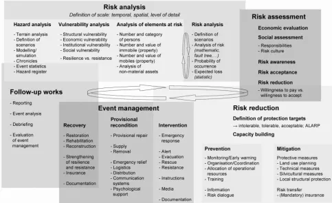
high-Figure 1.The model of integral risk management conceptualised as “risk cycle” (adapted from Carter, 1991; Alexander, 2000; Kienholz et al., 2004), based on an earlier version in www.nahris.ch and adapted from Fuchs (2009).
quality standards to provide for an integrated knowledge ba-sis for all relevant management options, including the design of appropriate mitigation measures and the policy implemen-tation during necessary decision-making actions.
Amongst others, integral risk management covers struc-tural (technical) measures for protection against nastruc-tural haz-ards. Aiming for the reduction of risk, they actively decrease hazard potential. For the case of torrential hazards, afforesta-tion measures, erosion control, check dams and levees are typically applied. If the damage potential is decreased, e.g. in terms of object protection, technical measures have a passive effect. Basically, hazard analysis by means of experimental and numerical modelling of relevant scenarios became in-creasingly important in the recent past. In the case of numer-ical modelling, significant advances in modelling techniques and the augmented computational power presently allow for analyses of complex issues and scenarios (e.g. Gems et al., 2014a, b; Mazzorana et al., 2014; Chiari, 2008). They enable the simulation of hazard processes on a large spatial scale (e.g. Gems, 2014c; Gems et al., 2012). Hydraulic scale mod-els are created mostly to address and model complex problem settings, geometrical configurations and compound scenar-ios, e.g. morphodynamics (sediment transport) in a complex three-dimensional flow field, flow–structure interaction and the bed load transport involved, and the impacts of hazard
processes on structures (e.g. Scheidl et al., 2013; Armanini and Scotton, 1992). Experimental modelling is restricted to a rather limited spatial scale.
a. A comprehensive methodology of vulnerability assess-ment requires a physics-based approach with a detailed representation of the impacting hazard process, both with respect to space and time.
b. Quantification of the resulting impacts on a building en-velope and detection of possible material intrusion pro-cesses require an analysis of the geometrical structure of the building with respect to the time-varying flow field of the impacting process and, if geo-mechanical actions may interfere, with respect to the residual bearing ca-pacity of the soil layers in which the object is situated. c. A physical response (resistance) analysis of the
build-ing structure considerbuild-ing the time-varybuild-ing impacts is re-quired, both, from a structural analysis perspective (stat-ics, elastostatics and dynamics) and a building physics viewpoint. Stresses and strains on the building have to be compared with maximum admissible values (accord-ing to the set of norms EN 1990 (Eurocode 0: Basis of Structural Design), EN 1991 (Eurocode 1: Actions on Structures) and the specific design codes EN 1992 to EN 1999).
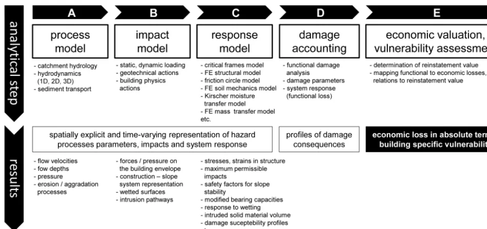
Referring to these basic requirements, Mazzorana et al. (2014) defined a five-step procedure according to Fig. 2 in order to reliably assess the physical vulnerability of el-ements at risk. The proposed concept is directed at unveil-ing the sequences of significant loss generation mechanisms, both methodologically and computationally. By evaluating potential damages, the scope of vulnerability assessment is expanded beyond its classical role as a decision-support tool and is closely linked to the planning process of torrent con-trol measures. The workflow requires the definition of a suit-able control volume and convenient control sections for ev-ery considered element at risk. Process and impact modelling (steps A and B according to Fig. 2) lead to a spatially explicit and time-varying quantification of actions and effects on the building structure. The response model (step C according to Fig. 2) consists of the verification of (i) a set of limit states according EN 1990 (ultimate limit states ULS and service-ability limit states SLS) and of (ii) the non-intrusion condi-tion for the liquid and solid material. Details on the steps of damage accounting and economic loss valuation are also covered in Mazzorana et al. (2012a, b, 2013).
Within the context of an analysis of a torrential hazard event, thereby explicitly focusing on the morphodynamic processes and not taking into account any geo-mechanical processes or the building’s physics, Mazzorana et al. (2014) applied the proposed concept for a residential building lo-cated at the alluvial cone of the Grossberg torrent in the Ital-ian Alps. The study highlighted the circumstance that for medium hazard intensities, vulnerability of buildings criti-cally depends on the patterns of water and material intrusion through openings such as doors, light shafts and windows. In addition to the proper consideration of the resistance of the
considered building in terms of the physical impact and the structural response, also the physical processes taking place on and throughout the building envelope (e.g. material in-trusion and moisture transfer and accumulation, wetting and drying of the outer and inner layers of the building) are found to be relevant within vulnerability assessment.
Due to a lack of data from fundamental research and soft-ware limitations, Mazzorana et al. (2014) neither consid-ered specific processes and analytical steps of the assessment scheme (Fig. 2) nor did they analyse them by using empirical data and models, mainly the following.
a. The transformation of process parameters (flow depths and velocities, bed level changes) to impact parame-ters (static and dynamic loadings) is based on straight-forward empirical approaches, estimating the impact of torrent hazards on idealised surfaces.
b. The processes of water and material intrusion and con-sequential impacts on the building envelope and on the damage pattern are not considered.
c. The economic valuation (damage estimation) is based on the application of empirical damage functions con-necting the loss to the maximum impacting flow depths. However, any dynamics and time-varying process pat-terns (wetting areas and durations, fluid forces, etc.) have some influence on the impact and response models and thus on the profiles of damage consequences. d. The applied case study explicitly considers one
spe-cific element at risk. Thus, and also due to the non-consideration of material intrusion processes, any inter-action of the relevant elements at risk situated on the Grossberg alluvial cone has not been analysed. Accord-ingly, also a geostatistical analysis focusing on the dam-age patterns and interaction of specific elements at risk situated at different spots on the alluvial cone has not been carried out.
In the context of the proposed procedure (based on Mazzo-rana et al., 2014), the present paper focuses on the hydrody-namic simulation of indoor flooding processes. A case study analysis is completed for a specific element at risk, situated close to a torrential stream in the Italian Alps. The flow field in the lower reach of the torrent channel, the flood plain in the near surroundings of the considered building and the build-ing’s flooding processes are modelled with the FLOW-3D software (Flow Science Inc., 2012), both for a set of steady and unsteady flow conditions. Regarding the aforementioned issues (a) to (c), mutual influences of the flow fields inside and outside of the building are analysed. Further, impacts on load-bearing walls of the building are evaluated discretely in space and time.
Figure 2.Proposed physics-based vulnerability assessment scheme according Mazzorana et al. (2014) (modified).
present case study analysis is a priori-constrained to pure wa-ter floods (WFL according to Heiser et al., 2015) and aimed mainly at the following research questions.
– If constraining to pure water floods (WFL) with no in-volvement of bed load (Heiser et al., 2015), is there a relevant dynamic impact of the entraining water on the building structure and a noticeable influence on the flow field on the surrounding flood plain?
– With regard to the planning process of local structural protection measures, does the simulation of building flooding processes provide any beneficial information? – From the perspective of computational capacity and
practical application, e.g. for flood plain mapping and hazard zone planning respectively, is it feasible to en-large the simulation area to a en-larger extent in order to cover a couple of buildings and objects?
2 Case study analysis
2.1 Introduction and modelling assumptions
Referring to the aforementioned introduction in vulnerabil-ity assessment and the consideration of mutual influences of flood hazard processes and buildings, the work presented within this paper deals with the simulation of building flood-ing processes, their influences on the adjacent flow field and the determination of impacting forces on a building struc-ture. In the sense of a case study analysis, focus is put on the flood plain at the Rio Vallarsa in the village of Laives (Au-tonomous Region of Trentino-Alto Adige, Italy, Fig. 3). One
specific element at risk, which is distinctly prone to flood-ing in the case of a torrential hazard event, is considered to be a permeable structure within hydrodynamic 3-D numeri-cal modelling (Fig. 5). Therein, solely impacts of pure wa-ter floods (WFL according Heiser et al., 2015) are analysed. Any expected influence of sediments, substantially (i) loss of flow capacity in the torrent channel due to the transport of bed load (Gems et al., 2014a, b; Hübl et al., 2002; Hun-zinger and Zarn, 1996), (ii) intrusion of sediments into the element at risk and (iii) a significant increase of impacting forces compared to clear water conditions (Mazzorana et al., 2014), are not considered.
The following two basic aspects support the disregard of bed load transport processes in this specific case.
a. Referring to the characteristics of the Rio Vallarsa catchment and the damage causing torrential hazard processes (Sect. 2.2), a deposition basin including a de-bris retention dam is located at the alluvial cone closely upstream the case study area (Fig. 3). The basin volume corresponds to the expected amount of sediment during a 150-year design event in the catchment. Bed load is not expected to pass the concrete dam; thus, the down-stream channel is loaded with pure water hydrographs only.
cur-Figure 3.(Left) overview of the Rio Vallarsa catchment and the Adige valley at the village of Laives (Italy); the colour scheme characterises an elevation model with a 2.5 m interval. (Right) track of the Rio Vallarsa torrent channel through settlement and commercial area in the south-western part of Laives; location of the case study area on the alluvial cone.
rently restricted to 2-D numerical codes (e.g. Vetsch et al., 2014; Rosatti and Begnudelli, 2013). This contrasts with the requirement of a three-dimensional approach, which is performed when the flow field is intended to be numerically modelled in- and outside of a complex building structure (featuring several floors and open-ings as doors, light shafts, windows, etc.). Further, from the perspective of computational demand, applications of 3-D numerical codes are basically limited to rather small river sections and small-scaled areas respectively (Gabl et al., 2014; Gems et al., 2014a; Habersack et al., 2007). Against this background, the presented case study analysis is intended to focus on a specific build-ing and its immediate sphere of influence. The simula-tions are aimed for use in the context of physics-based vulnerability analysis (Mazzorana et al., 2014) and the planning of local structural protection measures rather than large-scale inundation mapping. Thereby, subjects of investigation are also computational effort and limits of numerically modelling the building–fluid interaction, each from a practical perspective.
2.2 Catchment and building characteristics – hazard and damage potential
The Rio Vallarsa catchment is situated to the south of Bolzano (Italy). Covering 29.4 km2and ranging from 230 m at Laives to 1550 m above sea level, it represents a tribu-tary catchment to the Adige River. The catchment extends mainly in an east–west direction. From a geological per-spective, the catchment is shaped by the Bozen quartz por-phyry (in.ge.na engineering office, unpublished). In the up-per catchment part, marginal incisions in glacial deposits and gully erosion characterise the trunk torrent. A straight-line channel with moderate gradients and a few small tributaries can be observed in the middle part of the catchment. Fur-ther downstream, the Rio Vallarsa passes a raFur-ther narrow and
deeply incised canyon before entering the spacious Adige valley at the village of Laives. The torrent passes the set-tlement area of Laives on the south-west periphery along the border of the valley floor. After leading along the agricultural area, the channel enters the Adige River in the village of Ora. Both, fluviatile and debris flow regimes characterise ob-served torrential hazard events in the middle and upper catch-ment and as well the upper section on the alluvial cone (in.ge.na engineering office, unpublished; Fig. 3). Due to a sufficiently dimensioned sediment deposition basin at Laives (Fig. 3), flood discharges without significant fractions of sed-iment threaten the settlement and commercial areas further down the deposition basin (in.ge.na engineering office, un-published).
al-ready expected for discharges around HQ10 (Department of Hydraulic Engineering, Autonomous Province of Bolzano, unpublished). Buildings and infrastructure in close proxim-ity to the torrent channel are threatened of being flooded in the case of a torrential hazard event.
Figure 3 illustrates the situation at the southern part of the alluvial cone at Laives and the track of the Rio Vallarsa tor-rent. Therein, the case study area is situated straight down the deposition basin. It covers roughly 170 m of the trapezoidal rigid torrent channel, which features a gradient of 1.1 % and a cross section area of 19.5 m2. It is a brick work channel lined with cement mortar, whereby the channel side walls are par-tially covered with vegetation. The surrounding flood plain is further considered along this channel section. The main focus within numerical modelling is put on one specific building, situated orographically right in a distance of approximately 17 m to the channel.
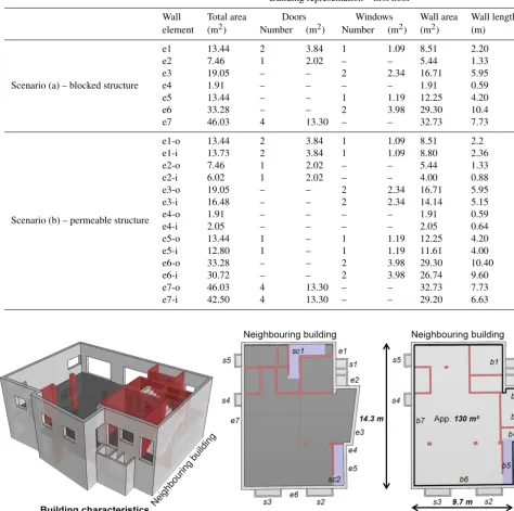
Figure 4 presents a perspective view of the considered building and shows top views of both, the building’s base-ment level and the first floor. With a floor area spanning ap-proximately 130 m2, the building features a rather complex structure, including a couple of potential openings for flood-ing, such as doors, light shafts and windows. With regard to the numerical model (Sect. 2.4) and the analysis of the simulation results (Sect. 2.5), the structural elements of the building are labelled accordingly. Further information on the structural elements of the building and the potential openings for indoor flooding processes is given in Sect. 2.3 (Table 1).
2.3 Hazard and building scenarios
A 300-year flood event is considered within hydrodynamic numerical modelling. In accordance with the reconstruction analysis of the flood event in November 2012 and further hy-drological catchment analyses (Department of Hydraulic En-gineering, Autonomous Province of Bolzano, unpublished), the corresponding peak discharge amounts to 120 m3s−1. The simulations are carried out in an unsteady mode, ap-proaching the expected 300-year flood hydrograph. Due to the computational effort, the simulations do not cover the entire design hydrograph. The investigation focuses on the rising limb of the design hydrograph, when the discharge ex-ceeds 30 m3s−1, and continue until the discharge falls below 30 m3s−1again in the falling limb. A discharge of 30 m3s−1 amounts to roughly 60 % of the HQ5 discharge and already leads to initial flooding of the cycle track at the bridge (Hofer, 2014). In order to keep the computational effort for the un-steady model simulations manageable, the simulation hydro-graph is chronologically scaled by a factor of 0.1 compared to the expected flood hydrograph under prototype conditions. With it, the computation time for the unsteady hazard sce-nario is 1020 s, and the total discharge volume entering the computational domain amounts to 720 270 m3.
Representing a preliminary study to this unsteady hazard scenario, steady-state simulations with the discharges 87 and
104 m3s−1and the 300-year peak discharge 120 m3s−1were also carried out. For this study, simulation results and any further details are presented by Hofer (2014). The discus-sion of the simulation results (Sect. 3.2) merely gives a very brief summary of it. Further, the influence of the simulation mode or rather the considered hazard scenario on the fluid– building interaction is analysed by qualitatively and quantita-tively comparing the results of the unsteady and steady-state simulations.
Concerning the implementation of the considered element at risk in the numerical model, three scenarios are analysed. Each is characterised by a certain degree of mutual influence between the building and the flow field on the surrounding flood plain. Scenario (a) treats the building as a fully blocked structure, not enabling any indoor flooding processes. The building envelope is thereby in accordance with the perspec-tive view in Fig. 4. All doors, light shafts and windows are permanently blocked. Table 1 illustrates the features of the wall elements e1–e7 on the first floor of the building envelope (Fig. 4). Concerning the listed wall areas, the dimensions of windows and doors are not included therein, although as-sumed to be closed for this scenario. Reflecting current stan-dard practice and methods in flood risk management and, more specifically, the consideration of buildings within inun-dation mapping (e.g. Tsakiris, 2014; Habersack et al., 2007), scenario (a) with a fully blocked building represents the ref-erence case for further scenarios.
With scenario (b), the building is treated as a permeable structure. All openings are set permanently and entirely open. This assumption runs contrary to scenario (a); however, it does also not fully conform to typical natural conditions. Also for scenario (b), the features of the wall elements (first floor) are listed in Table 1. In this case, wall surfaces in-side the building and on the outin-side are separately consid-ered with components each in the numerical model in order to allow for an individual analysis of wetted areas and fluid forces acting on the walls.
As shown in the perspective view in Fig. 4, the building features a couple of openings on its south-west and west sides, both directly facing to the Rio Vallarsa channel. Deal-ing with the efficacy of local structural protection measures, scenario (c) further considers specific permanent modifica-tions at the building, which are intended to reduce or best possibly prevent the fluid from flooding critical spots within the building. There, the light shafts s1, s4 and s5 (Fig. 4) are closed with a cover and the top levels of the light shafts s2 and s3 are raised by 0.8 m to a level which is expected to overtower the critical flow depth on the surrounding flood plain. Remaining openings of the building envelope are con-sidered to be open, which is in accordance with the setting of scenario (b).
Table 1.Building representation for the considered scenarios (a), with a fully blocked structure, and (b), assuming all doors, light shafts and windows to be entirely open; wall element notations refer to Fig. 4; for scenario (b), index “o” means the outside of the wall element, and “i” refers to the inside.
Building representation – first floor
Wall Total area Doors Windows Wall area Wall length element (m2) Number (m2) Number (m2) (m2) (m)
Scenario (a) – blocked structure
e1 13.44 2 3.84 1 1.09 8.51 2.20
e2 7.46 1 2.02 – – 5.44 1.33
e3 19.05 – – 2 2.34 16.71 5.95
e4 1.91 – – – – 1.91 0.59
e5 13.44 – – 1 1.19 12.25 4.20
e6 33.28 – – 2 3.98 29.30 10.4
e7 46.03 4 13.30 – – 32.73 7.73
Scenario (b) – permeable structure
e1-o 13.44 2 3.84 1 1.09 8.51 2.2
e1-i 13.73 2 3.84 1 1.09 8.80 2.36
e2-o 7.46 1 2.02 – – 5.44 1.33
e2-i 6.02 1 2.02 – – 4.00 0.88
e3-o 19.05 – – 2 2.34 16.71 5.95
e3-i 16.48 – – 2 2.34 14.14 5.15
e4-o 1.91 – – – – 1.91 0.59
e4-i 2.05 – – – – 2.05 0.64
e5-o 13.44 1 – 1 1.19 12.25 4.20
e5-i 12.80 1 – 1 1.19 11.61 4.00
e6-o 33.28 – – 2 3.98 29.30 10.40
e6-i 30.72 – – 2 3.98 26.74 9.60
e7-o 46.03 4 13.30 – – 32.73 7.73
e7-i 42.50 4 13.30 – – 29.20 6.63
Figure 4.Object of investigation within 3-D hydrodynamic modelling – (left) perspective view and (middle, right) top views of first floor and basement level; notations e1–e7 identify exterior walls on the first floor, b1–b7 denote to corresponding wall elements on the basement level; inner walls are coloured red, s1–s5 characterise light shafts and sc1–sc2 identify stair cases (coloured blue).
the building with the measures tested in scenario (c) is not expected.
For all building scenarios (a), (b) and (c), both the steady-state events and as well the unsteady torrential hazard sce-nario are computed.
2.4 Numerical model
scheme and a perspective view of the FAVOR-model (Flow Science Inc., 2012) are illustrated in Fig. 5.
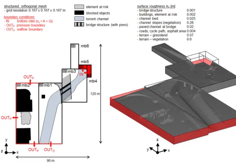
The computational domain, basically covering the section of the brick work channel of the Rio Vallarsa (Sect. 2.2) and the surrounding flood plain orographically right to the channel, is meshed with six structured, orthogonal mesh blocks (mb). The grid resolution is equally set to 0.167 m×0.167 m×0.167 m for every mesh block. The in-put boundary is defined as a bottom inlet, represented by two small and accurately defined areas at the upstream model boundary and inflow velocities in a positive vertical direc-tion. At the model outlets on the flood plain, pressure bound-ary conditions are set, each with the assumption that unreal-istic backwater effects can be excluded. As illustrated in the model scheme in Fig. 5, pressure boundary conditions are set at the Xmin, Ymin and Ymax boundary of mesh block mb2. At the downstream edge of the channel, the boundary condition “outflow”, coping best with a varying discharge at the un-gaged model boundary (Hofer, 2014), is applied. Con-cerning both, the grid resolution and the boundaries, com-prehensive tests on their influence on the flow field within the computational domain have been carried out by Hofer (2014), amongst simulations with uniform grid resolutions of 0.33, 0.167 and 0.25 m. Related to the modelling results with the grid size of 0.167 m, relative differences in flow depths and velocities of 1.75 % and 10 % at maximum in the chan-nel were analysed. Mesh refining from a grid size of 0.167 to 0.125 m increased the computation times by a factor of 5. An influence of the grid resolution on the model stability was not observed thereby and the adaptive (and in FLOW-3D inter-nally controlled) computational time step decreased with in-creasing grid resolution. Therefore, with regard to accuracy and computational effort, the mentioned grid resolution of-fers an optimal compromise (Hofer, 2014). Mesh block mb6 is set due to the fact that in the case of higher discharges, the flow enters also the cycle path in the near range of the bridge. Mesh block mb6 allows for a spreading along the cycle path towards upstream without reaching the Ymax boundary of the mesh block.
The considered building is situated within mesh block mb2. Depending on the considered building scenario (Sect. 2.3), it is modelled as blocked or permeable structure or rather a structure with local structural protection measures. In order to individually analyse wetted areas and force mag-nitudes on the wall elements, every element is implemented as an individual component in the model. Further, to distin-guish between impacts inside the building and on the outside, the wall elements of the first floor are modelled with two components each, partially overlapping each other and shap-ing the wall structure together (Hofer, 2014). The remainshap-ing buildings and objects are modelled as blocked objects. The 3-D numerical model contains 7.05 million cells. Thereof, 2.65 million cells represent active cells for the simulation (for sce-nario b).
With regard to a plausibility check of the numerical mod-elling results and, thereby, an appropriate definition of addi-tional roughness parameters for the channel section and the flood plain, no flood events have been observed in the re-cent past that caused relevant flooding or damages in the case study area. As already stated in Sect. 2.3, the peak discharge 55 m3s−1, observed in November 2012, caused bankfull flow conditions in the channel. This information was used for the calibration of the numerical model of the channel geom-etry by adjusting the corresponding roughness parameters. The model thus leads to overbank flooding at discharges of about 60 m3s−1(Hofer, 2014), and this adequately fits with available information and expert assessment (Department of Hydraulic Engineering, Autonomous Province of Bolzano, unpublished). Since any observation data is not available on the flood plain and for the building structure, roughness parameters are set to characteristic values commonly cited in the literature (e.g. Giesecke et al., 2014; Landesanstalt für Umweltschutz Baden-Württemberg, 2002). The spatial extent of specific surface structures and vegetation is ade-quately considered thereby. The chosen additional roughness coefficients are mentioned in Fig. 5.
Concerning the turbulence options in the numerical simu-lations, the standard two-equation k––turbulence model is set.
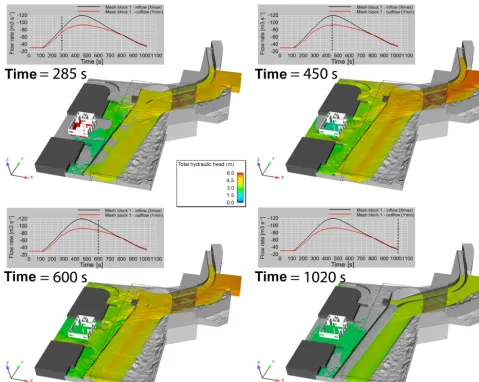
2.5 Results of unsteady hydrodynamic modelling Figure 6 illustrates snap shots of the simulation for scenario (b) with the assumption of a permeable building envelope. Perspective views of the computational domain at four dif-ferent time frames are pictured. The colouring of the fluid isosurface denotes to the total hydraulic head, which in-cludes water depth and velocity head. The isosurface value is thereby set to 0.25 in order to illustrate very low water depths on the outer channel embankment. Further, the flow rates at the channel in- and outflow of mesh block mb1 (Fig. 5) point out the maximum discharge capacity in the channel and the fluid volume impacting the adjacent flood plain. Negative flow rates at the mesh block boundaries are due to the ori-entation of the coordinate system set for the computations.
Figure 5.(Left) scheme of the hydrodynamic numerical model; (right) computational model representation with the FAVOR-method (Flow Science Inc., 2012).
side opposite to the channel via the light shafts s4 and s5 from the basement level and the openings of wall element e7 on the first floor. Within the falling limb of the hydro-graph, the flow depths in the building and on the surrounding flood plain decrease again. However, the basement level of the building remains fully filled up to the level of the ceiling of the storey in question. It should be noted that the storey ceiling is not figured out in Fig. 6, it is of course considered within numerical modelling. Wall elements of the basement level are coloured red in Fig. 6. Those of the first floor have a white colour.
To give a further impression on the characteristics of in-flux into in the building structure and flow conditions inside, Fig. 7 illustrates depth averaged velocities at sections in the directions of thexand theyaxis, again for scenario (b). With the section in the direction of theyaxis as a spatial reference, streamlines depict main flow paths at different time frames during simulation. A rather turbulent and temporarily signif-icantly changing flow pattern characterises the situation in-side the building. Initially, as long as the basement level is not entirely filled, the fluid enters the building mainly via light shaft s3 and the flow field in the building has a distinc-tive rotational character. As simulation time progresses, the
flow pattern becomes more and more disordered and flow in both directions occurs at the openings of the building enve-lope as well as on the inside.
Initially, maximum depth averaged velocities up to 5 ms−1 occur inside the building. These maxima are spatially limited to the vertical drops at the light shafts. Subsequently and, if focusing on the conditions on the basement level, with in-creasing filling ratio of the building volume, flow velocities significantly decrease and approach almost zero values.
Figure 6.Modelling results for scenario (b) after 285, 450, 600 and 1020 s of simulation – perspective view of the stl-geometries and the fluid isosurface representing the total hydraulic head (m), boundary flow rates (Xmax, Ymin) for mesh block mb1.
are analysed. Results for scenario (a) are coloured in black, the colour red is assigned to the results for scenario (b).
Concerning the peak ratios, there is only a marginal dif-ference between the scenarios (a) and (b). A maximum wet-ting percentage of roughly 25 % occurs at wall element e1 for both scenarios, the peaks at e5, e6 and e7 are 50 %, 50 % and 7.5 % accordingly. The comparatively low wetted areas at the outside of wall element e7 are due to the fact that it is oriented to the south of the building and thus not directly exposed to the flow.
However, some significant differences between the two scenarios (a) and (b) can be observed in the temporal devel-opment of wetting. In the case of scenario (a), flow on the almost flat flood plain is prevented from entering the build-ing at the light shafts (s2 and s3). The wettbuild-ing ratio at wall element e6 on the short side of the building features signifi-cantly higher values during the rising limb of the flood hy-drograph. The plateau in the red line for wall element e6
until the time frame of 450 s marks the filling progress of the basement level. Once completely filled, water accumu-lates at the outside of wall element e6 and the wetting ratio increases rapidly. There is no significant difference at wall element e6 between the scenarios during the falling limb of the hydrograph, except for a marginal lower water level for scenario (b) at the end of the simulation. The same holds for the characteristics of wetting at wall element e5 on the build-ing side facbuild-ing the Rio Vallarsa channel. In accordance to the situation at wall element e6, e1 is also impacted more sig-nificantly during the rising limb of the hydrograph. Due to the blockage of the building, damming on the flood plain ap-pears earlier, and the flow depths at wall element e1 increase accordingly.
Figure 7.Scenario (b) after 350, 450, 600 and 1020 s of simulation – 2-D sections and streamlines with depth averaged velocity contours (m s−1), illustrating flow paths and characteristics of in- and outflow of the building (stl-geometry of the building).
openings of wall element e7. With it, the relative difference in wetting between both scenarios is highest at the building en-velope not facing the Rio Vallarsa channel. With regard to the comparison in the block diagrams, durations with lower wet-ting ratios are on an average higher for scenario (b), whereas higher wetting ratios are lower. This holds for the wall ele-ments e1, e5 and e6.
On the basis of the hydraulics at the building, the dynami-cally impacting fluid forces are analysed in Fig. 9, left. Force magnitudes at the first-floor-wall elements e1–e7 are com-pared for the scenarios (a) and (b). Concerning scenario (b), the impacts in- and outside the building are plotted individu-ally (red dots in Fig. 9, left). Force magnitudes are calculated
from the temporarily varying pressure and shear forces; they represent the maximum total force on the wall element within the entire simulation period.
Figure 8.(Top line) ratio of wetted and total area of the wall elements e1, e5, e6 and e7 at the outside of the building for the scenarios (a) and (b); (lower line) comparison of wetting durations (number of time steps à 10 s) for the considered wall elements.
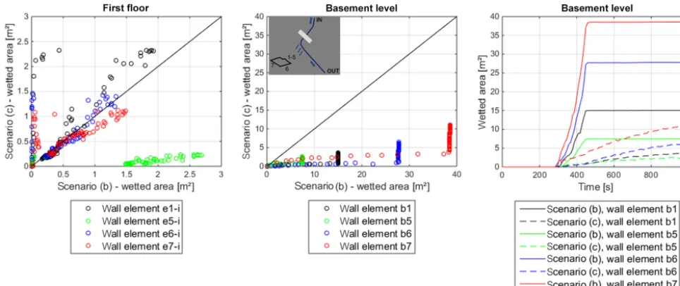
Figure 9. (Left) fluid force magnitudes (kN) on the building envelope for the scenarios (a) and (b); (middle) wetted areas of wall ele-ments (m2) inside the building for scenario (b); (right) specific fluid force magnitudes (kN m−2) at wall elements on the basement level for scenario (b).
This is mainly due to the facts that (i) the fluid firstly fills the basement level and only insignificantly impacts the first floor at the inside at the beginning of the flooding and (ii) the force components due to the dynamics of the fluid (lower veloci-ties) are comparatively lower.
With regard to scenario (b), Fig. 9 further shows the wetted area in function of the time each for the wall elements e1-i, e5-i, e6-i and e7-i on the first floor and the corresponding wall elements on the basement level. Concerning the latter, wetting ratios reach a value of 1.0 after 450 s of simulation and remain constant until the end of simulation. Due to the characteristics of the building structure, wetting on the first
Figure 10.Comparison of wetted areas (m2) during the simulations of the scenarios (b) and (c) – (left) wall elements e1, e5, e6, e7 on the first floor inside the building; (middle) wall elements b1, b5, b6 and b7 on the basement level (simulation results with output time steps à 10 s); (right) temporal characteristics of wetting for the wall elements on the basement level for the scenarios (b) and (c).
If changing the opening characteristics of the building, the fluid impact inside the building is significantly different, not necessarily going along with an exclusive decrease of im-pacts if specific local structural protection measures are built. This aspect is shown in Fig. 10 by means of a comparison of the scenarios (b) and (c). Wetted areas of the wall elements e1-i, e5-i, e6-i and e7-i on the first floor are compared (left diagram). The situation on the basement level is shown in the middle and left diagram.
In the case of scenario (c), the process of flooding the building occurs in a way other than for scenario (b): The ini-tial fluid influx via the light shafts is disabled due its covering and raise. The fluid enters the building through the doors and windows on the first floor, stays and spreads in the building and partially leaves again. The basement level is filled from the fluxes inside via the staircases; it does not get fully filled during the entire simulation period. Accordingly, wetted ar-eas and impacting forces on the basement level are signif-icantly lower for scenario (c) than for scenario (b). Higher impacts occur for scenario (c) on the first floor, except for wall element e5 on the building side facing the Rio Vallarsa channel. This wall element is affected only marginally due to the facts that the bordering staircase sc2 is placed directly in front and the fluid on the basement level does not reach the storey ceiling. Within this context it has to be noted that the scenarios (b) and (c) do not fully accurately represent the pure natural behaviour of the building in the case of flooding. Doors and windows are assumed to be fully open during the entire duration of the flood hydrograph. At real conditions, if not protected with specific sealing and reinforcement fea-tures, they are expected to have neither a full blocking nor
an open but a partially permeable effect. However, simula-tion scenario (c) highlights the need of an excellent plan-ning procedure for building hazard-proof buildings in order to achieve efficient and reliable flood protection.
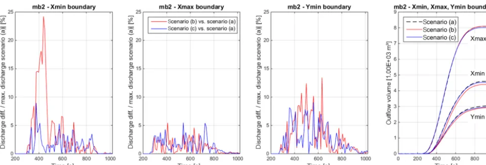
Whereas from a building’s durability point of view the im-pact of flooding is of basic relevance, the way of considering a certain element at risk within numerical modelling seems to insignificantly influence the flow field on the surrounding flood plain. To give an impression on this process of mu-tual influence, Fig. 11 illustrates time-dependent flow data at the boundaries of mesh block mb2. The differences of dis-charges between scenarios (b) and (a) (red lines in Fig. 11, left and middle) and as well between scenarios (c) and (a) (blue lines in Fig. 11, left and middle) are related to the max-imum boundary outflow for scenario (a) and plotted as abso-lute values against time at the boundaries Xmin, Xmax and Ymin of mesh block mb2. Mesh block mb2 covers the flood plain orographically right to the channel (Fig. 6) where a cer-tain influence of the building is expected.
Figure 11.Discharges at the boundaries Xmin, Xmax and Ymin of mesh block mb2 (Fig. 5) – (left and middle) time-dependent discharge differences between scenario (b) and (a) in relation to the maximum discharge of scenario (a) at the considered boundaries; (right) scenario-specific outflow volumes at the boundaries.
of the flood hydrograph (720 270 m3), a total of 2.1 % passes the boundaries of mesh block mb2 for scenario (a). A com-parison of the scenarios with each other reveals volume ratios within the range 0.9579–1.0002.
Differences in flow parameters (water depths, velocities) between the considered building scenarios are as well small, except for the area inside the building and very close to the building envelope. They are considerably smaller within the computational domain than at the model boundaries.
3 Discussion and conclusions
3.1 Fluid–building interaction – general relevance of indoor flooding processes under clear water conditions
The results of hydrodynamic numerical modelling (Sect. 2.5) show a rather marginal influence of the building on the flow field on the flood plain and in the Rio Vallarsa channel. Due to the small interior volume of the building compared to the volume of the simulated flood hydrograph, this behaviour is more or less independent from the way of considering the el-ement at risk within the simulation model (Fig. 11). If not for scaling the expected hydrograph (by a factor of 0.1 in order to cope with the computational effort) and perfectly simu-lating real conditions, this influence would be considerably smaller.
Otherwise, focusing on the impact of the fluid on the inside of the building, a certain impact can be observed. This im-pact on the inside is mainly characterised by relatively small flow velocities (Fig. 7) but long wetting durations that ba-sically extend beyond the duration of the hazard event. The impact (Fig. 9) does not threaten the stability of the build-ing (limit states ULS accordbuild-ing EN 1990, Sect. 1) but affects the building physics and, with it, the usability (limit states
SLS according EN 1990, Sect. 1). The latter may cover also potential serious damage of electrical and in-house installa-tions, furnishing and equipment. This kind of damage will be considerably higher under real conditions, when fine sed-iments (suspended load) that pass the debris retention dam, contribute also and get deposited inside the building. A sig-nificant impact on the stability of the building probably re-quires the contribution and consideration of conditions with intense sediment loads (WST and DBF according Heiser et al., 2015) or rather the modelling of geo-mechanical pro-cesses (Sect. 1).
However, with regard to the danger to life and limb inside buildings, numerical modelling under clear water conditions is highly valuable. The characteristics of flooding the build-ing provide information for evacuation plannbuild-ing or rather non-affected areas during hazard events.
3.2 Fluid–building interaction with different
hydrological modelling scenarios – comparison of an unsteady and a steady-state modelling approach The simulation results presented in Sect. 2.5 exclusively focus on the unsteady hydrological scenario, specified as 300-year torrential hazard and design event for flood risk management (Sect. 2.4). The present computational domain and element at risk was already studied by Hofer (2014) in terms of a steady-state analysis of specific hazard scenarios. Hofer (2014) simulated specific discharges up to 120 m3s−1 and analysed wetted areas and impacts on the considered building at the end of each simulation when steady-state con-ditions were achieved within the computational domain. Cri-teria for the steady-state condition were thereby mainly fo-cused on the fluxes at the mesh block boundaries. In anal-ogy with the unsteady modelling approach, the three building scenarios (a), (b) and (c) were analysed (Sect. 2.3).
When qualitatively comparing the results of the two dif-ferent modelling approaches and reflecting the propagation of flooding in the unsteady scenario simulation, the process of filling the interior volume of the building can obviously not be adequately modelled with a steady-state simulation. The basement level of the building is getting fully filled up until the end of steady-state simulation independently from flood discharge, only the required simulation time changes accordingly. As the evaluation of results is carried out solely at the end of the steady-state simulations when the maximum fluid impacts are supposed to appear, this presumed “unnatu-ral” process of filling the building certainly distorts the mod-elling results. Depending on the characteristics of the design flood (discharge volume), the retention effect of the con-sidered building is thereby either under- or overestimated: An underestimation is observed at conditions in which the considered building is in fact flooded, but the duration of overbank flooding within unsteady modelling is less than the steady state modelling duration. An overestimation possibly appears at conditions with very short durations of overbank flooding and impacting, as a steady state model, assuming a constant peak discharge, unnaturally extends these dura-tions. This statement is further underpinned by the fact that, with the unsteady simulations, maximum potential impacts may appear also at conditions, when both the basement level and the first floor of the building are filled but the water level on the basement level does not necessarily reach the storey ceiling (Figs. 6 and 8). The time of maximum impacts is thus mainly dependant on the characteristics of the flood hydro-graph. Further, with regard to an analysis of expected wetting durations (Fig. 8), a steady-state modelling approach does not allow any conclusions. Against this background, differ-ences in fluid impacts resulting from unsteady and steady-state modelling are observed mainly for scenarios, where in-door flooding actually appears to a rather less extent. This is the case for scenario (c) for example. Consideration of vol-ume of the flood hydrograph seems at least equally important
as the flood peak. Further, the differences of the results for the three considered building scenarios are less pronounced with the steady-state simulations.
A qualitative comparison of the steady-state and the un-steady modelling results reveal an underestimation of the im-pacts on the building for the steady-state simulations with the 120 m3s−1 discharge. Further details and results of the steady-state simulations can be found in Hofer (2014).
Irrespective of the capabilities and constraints of both modelling approaches, it has to be noted that the steady-state simulations require a substantially lower computational ef-fort. This is due to shorter simulation times leading up until the simulations reach steady-state conditions compared to the duration of the discharge hydrographs.
Summarising, the applicability of the steady-state mod-elling approach is reasonable in the context of preliminary studies with the objective of verifying the general appearance of indoor flooding processes for specific hydrological condi-tions or analysing the effects of local structural protection measures in terms of entirely preventing indoor flooding.
3.3 Computational modelling effort – capabilities and limits for practical application in flood risk management
Under given effort of hydrodynamic numerical modelling and with consideration of the illustrated intensity of the fluid–building interaction (Sects. 2.5, 3.1 and 3.2), the basic question, whether there is any sense in considering indoor flooding processes in practical application, arises. Figure 12 provides performance details from the unsteady numerical calculations. The left diagram shows the computation times for the scenarios (a), (b) and (c), each in relation to the sim-ulation time. Accordingly, the middle diagram presents the applied time step sizes and the diagram on the right points out the computation times per time step in relation to the sim-ulation time.
Basically, all accomplished computations require long computing times compared to the simulation time or rather real time conditions. With the use of an Intel core i7-3820 quad-core processor (@ 3.60 GHz), 32 GB main memory and a parallel software license code, computation times of about 200 h are achieved for the scenarios (a) and (b), without any substantial differences between these scenarios. The time step sizes generally decrease with the occurrence of flood-ing and spreadflood-ing on the flood plain. The computation time per time step features an almost linear relation to the fluid surface area within the computational domain, again with an insignificant influence of the building flooding process.
Figure 12.Computational effort – comparison of computation time (h) (left), time step size (1.0 E-3 s) (middle) and computation time per time step (s) (right) for the scenarios (a), (b) and (c).
The flow on these fine-structured, stepped obstacles leads to an adjustment of the time step size.
In a more general sense, 3-D hydrodynamic modelling of flood hydrographs and the spreading on a flood plain is a very time-consuming task, even though rather small compu-tational domains (0.564 ha in this study) are analysed. The computational effort can but does not necessarily have to further increase if building flooding processes are consid-ered. This statement is underpinned by the fact that for the unsteady scenario simulation the expected design flood was adapted by a scale factor of 0.1 (Sect. 2.3) in order to achieve manageable computation times. Practical application in flood risk mapping, typically covering a larger extent of the flood plain and at least a couple of elements at risk, seems to not be practicable (or mandatory) in this context. Compared to the rather small influence of a permeable building structure on the flow field on the surrounding flood plain, a potential significant increase of computation time is furthermore not reasonable.
However, for vulnerability analysis and the planning of local structural protection measures for specific elements at risk, the modelling of building flooding processes means a valuable tool. Specific planning options can be tested and verified on their efficiency. They can be further compared with each other within a cost–benefit analysis where poten-tial hazard impacts or rather avoided impacts and damages are considered. Compared to the general expense of the plan-ning process and, for the case of an insufficient efficiency of the measures due to a poor planning, to the extent damages, the costs for numerical modelling and scenario simulation is perfectly acceptable.
4 Aspects of further research
The assessment of the specific vulnerabilities of the built en-vironment is the pillar for any planning process that is
tar-geted at a reduction of the expected adverse consequences. These adverse consequences result from the interactions be-tween the hazard processes and the exposed elements, both in time and space. From a physical perspective, these interac-tions firstly take the form of damage-generating mechanisms, which are quantifiable knowing the hazard intensities and the physical response of the structures in terms of (i) deforma-tions with respect to the admissible states, (ii) the wetting process of the buildings envelope and its alterations. Given specified loading conditions and determined geometrical and material properties of the building envelope, the subsequent mass transport processes through it may result in secondary damage-generating mechanisms.
This work represents a step towards the development of a comprehensive physical vulnerability assessment frame-work and shows how advanced modelling techniques may be usefully employed for pure water floods. However, fur-ther research efforts are needed (i) to develop reliable and practicable 3-D codes for the whole spectrum of flow pro-cesses involving sediment transport at various rates and fea-turing different non-Newtonian flow behaviours, (ii) to cou-ple the simulation of flow dynamics with structural mechan-ics. In parallel, if the aforementioned advances are feasible, it is fundamental to provide for effective, easy handling and cheap methods as terrestrial photogrammetry to create high-resolution building models. Additionally, it is essential to op-timize the physical parameterization (i.e. material properties) of such models. In this context, physical scale model experi-ments could provide novel and valuable insights.
Self-evidently, only a limited number of key elements of the built environment should be analysed to such a level of detail; therefore a harmonisation with the available vulnera-bility information for the remaining exposed elements is nec-essary.
mitigation strategy. Conceiving vulnerability as a continuum along the risk cycle with respect to both, space and time, con-siderable efforts should be devoted to significantly enhance the societal capacities to cope with and recover from the re-maining adverse effects of occurring flood events. Last but not least it is essential that post-event design processes aim at reconfiguring the flood prone system by avoiding serious damage-generating mechanisms and not at reconstructing the elements of the built environment featuring the same old set of vulnerabilities.
Acknowledgements. The presented study was completed at the Uni-versity of Innsbruck and in close collaboration with the Department of Hydraulic Engineering of the Autonomous Province of Bolzano. The Unit of Hydraulic Engineering thanks the Department of Hy-draulic Engineering for this precious cooperation. Further thanks are due to the owner of the modelled element at risk for providing highly valuable plan documents of the building structure and expe-rience of flood event characteristics, and, most notably, for keeping an open mind for scientific research.
The presented study was conducted during the review stage of a 3-year research project, funded by the Austrian Science Fund (FWF): P 27400-NBL. It provides valuable information on capabil-ities and limitations of numerically modelling the process-building interaction.
Edited by: K. Schröter
Reviewed by: two anonymous referees
References
Alexander, D. E.: Confronting Catastrophe: New Perspectives on Natural Disasters, Harpenden, UK and New York, Terra and Ox-ford University Press, p. 5, 2000.
Armanini, A. and Scotton, P.: Experimental analysis on the dynamic impact of a debris flow on structures, Proceedings of the Inter-praevent 1992, Bern, Vol. 6, 107–116, 1992.
Carter, W. (Ed.): The disaster management cycle, Disaster manage-ment: a disaster manager’s handbook, Manila, Philippines: Asian Development Bank, 51–59, 1991.
Chiari, M.: Numerical Modelling of Bedload Transport in Torrents and Mountain Streams, doctoral thesis, Institute of Mountain Risk Engineering, University of Natural Resources and Life Sci-ences Vienna (BOKU), 2008.
Department of Hydraulic Engineering, Autonomous Province of Bolzano – South Tyrol: Ricostruzione dell’evento del 11.11.2012, unpublished.
Fell, R., Corominas, J., Bonnard, C., Cascini, L., Leroi, E., and Sav-age, W.: Guidelines for landslide susceptibility, hazard and risk zoning for land-use planning, Eng. Geol., 102, 85–98, 2008. Flow Science Inc.: FLOW-3D, v10.0, user manual, 2012.
Fuchs, S.: Susceptibility versus resilience to mountain hazards in Austria – paradigms of vulnerability revisited, Nat. Hazards Earth Syst. Sci., 9, 337–352, doi:10.5194/nhess-9-337-2009, 2009.
Fuchs, S.: Mountain hazards, vulnerability, and risk – a contribution to applied research on human-environment interaction.
Habilita-tion thesis at the University of Innsbruck, Austria, 2009, unpub-lished.
Fuchs, S., Heiss, K., and Hübl, J.: Towards an empirical vulner-ability function for use in debris flow risk assessment, Nat. Hazards Earth Syst. Sci., 7, 495–506, doi:10.5194/nhess-7-495-2007, 2007.
Gabl, R., Gems, B., De Cesare, G., and Aufleger, M.: Anregungen zur Qualitätssicherung in der 3-D-numerischen Modellierung mit FLOW-3D, WasserWirtschaft – Fachzeitschrift für Wasser und Umwelttechnik 03/2014, 15–20, doi:10.1365/s35147-014-0938-0, 2014.
Gems, B.: Entwicklung eines integrativen Konzeptes zur Mod-ellierung hochwasserrelevanter Prozesse und Bewertung der Wirkung von Hochwasserschutzmaßnahmen in alpinen Talschaften – Modellanwendung auf Basis einer regionalen Betrachtungsebene am Beispiel des Ötztales in den Tiroler Alpen Forum, doctoral thesis, Unit of Hydraulic Engineering, University of Innsbruck, Innsbruck University Press (IUP) (= Forum Umwelttechnik und Wasserbau, 13), 2012.
Gems, B., Wörndl, M., Gabl, R., Weber, C., and Aufleger, M.: Ex-perimental and numerical study on the design of a deposition basin outlet structure at a mountain debris cone, Nat. Hazards Earth Syst. Sci., 14, 175–187, doi:10.5194/nhess-14-175-2014, 2014a.
Gems, B., Sturm, M., Vogl, A., Weber, C., and Aufleger, M.: Anal-ysis of damage causing hazard processes on a torrent fan – scale model tests of the Schnannerbach Torrent channel and its entry to the receiving water, Digital Proceedings of the Interpraevent 2014 in the Pacific Rim, Nara, 2014b.
Gems, B., Sturm, M., Aufleger, M., and Neuner, J.: Reconstruc-tion of event-related bed-load transport processes in alpine catch-ments – application of TomSed on a large spatial scale, in: River Flow 2014, edited by: Schleiss, A. J., de Cesare, G., Franca, M. J., and Pfister, M.: Proceedings of the 7th International Confer-ence on Fluvial Hydraulics, London, Taylor & Francis, ISBN 978-1-138-02674-2, 941–949, 2014c.
Giesecke, J., Heimerl, S., and Mosonyi, E.: Wasserkraftanla-gen – Planung, Bau und Betrieb, 6. aktualisierte und er-weiterte Auflage, Springer-Verlag Berlin Heidelberg, p. 204, doi:10.1007/978-3-642-53871-1, 2014.
Habersack, H., Hengl, M., Knoblauch, H., Reichel, G., Rutschmann, P., Sackl, B., and Tritthart, M.: Fließgewässermod-ellierung – Arbeitsbehelf Hydrodynamik; Grundlagen, Anwen-dungen und Modelle für die Praxis, ÖWAV-Arbeitsbehelf, 37, 2007.
Heiser, M., Scheidl, C., Eisl, J., Spangl, B., and Hübl, J.: Process type identification in torrential catchments in the eastern Alps, Geomorphology, 232, 239–247, 2015.
Hofer, T.: 3D-numerische Modellierung der Durch- und Umströ-mung von Infrastrukturobjekten (Gebäuden), master thesis, Unit of Hydraulic Engineering, University of Innsbruck, 2014. Holub, M., Suda, J., and Fuchs, S.: Mountain hazards: reducing
vul-nerability by adapted building design, Environ. Earth Sci., 66, 1853–1870, doi:10.1007/s12665-011-1410-4, 2012.
Engineer-ing, University of Natural Resources and Applied Life Sciences, Vienna, 2002.
Hufschmidt, G.: A comparative analysis of several vulnerability concepts, Nat. Hazards, 58, 621–643, 2011.
Hunzinger, L. and Zarn, B.: Sediment Transport and Aggradation Processes in Rigid Torrent Channels. Proceedings of the Inter-praevent 1996, Garmisch-Partenkirchen, Vol. 4, 221–230, 1996. in.ge.na engineering office: Hydrogeologischer
Gefahrenzonen-plan, Gemeinde Leifers – Ausführlicher Bericht Wasserge-fahren/Piano delle zone di pericolo idrogeologico, commune di Laives – Relazione dettagliata pericoli idraulici, unpublished. Kappes, M., Keiler, M., von Elverfeldt, K., and Glade, T.:
Chal-lenges of analyzing multi-hazard risk: a review, Nat. Hazards, 64, 1925–1958, 2012a.
Kappes, M., Papathoma-Köhle, M., and Keiler, M.: Assessing physical vulnerability for multihazards using an indicator-based methodology, Appl. Geogr., 32, 577–590, 2012b.
Kienholz, H., Krummenacher, B., Kipfer, A., and Perret, S.: As-pects of integral risk management in practice – considerations with respect to mountain hazards in Switzerland, Österreichische Wasser und Abfallwirtschaft, 56, 43–50, 2004.
Landesanstalt für Umweltschutz Baden-Württemberg: Hydraulik naturnaher Fließgewässer, Teil 2 – Neue Berechnungsverfahren für naturnahe Gewässerstrukturen, 1. Auflage, Karlsruhe, 47–49, 2002.
Mazzorana, B., Levaggi, L., Formaggioni, O., and Volcan, C.: Phys-ical vulnerability assessment based on fluid and classPhys-ical me-chanics to support cost-benefit analysis of flood risk mitigation strategies, Water, 4, 196–218, doi:10.3390/w4010196, 2012a. Mazzorana, B., Levaggi, L., Keiler, M., and Fuchs, S.: Towards
dy-namics in flood risk assessment, Nat. Hazards Earth Syst. Sci., 12, 3571–3587, doi:10.5194/nhess-12-3571-2012, 2012b. Mazzorana, B., Comiti, F., and Fuchs, S.: A structured approach
to enhance flood hazard assessment in mountain streams, Nat. Hazards, 67, 991–1009, 2013.
Mazzorana, B., Simoni, S., Scherer, C., Gems, B., Fuchs, S., and Keiler, M.: A physical approach on flood risk vulnera-bility of buildings, Hydrol. Earth Syst. Sci., 18, 3817–3836, doi:10.5194/hess-18-3817-2014, 2014.
Papathoma-Köhle, M., Kappes, M., Keiler, M., and Glade, T.: Phys-ical vulnerability assessment for alpine hazards: state of the art and future needs, Nat. Hazards, 58, 645–680, 2011.
Papathoma-Köhle, M., Keiler, M., Totschnig, R., and Glade, T.: Improvement of vulnerability curves using data from extreme events: debris flow event in South Tyrol, Nat. Hazards, 64, 2083– 2105, 2012.
Rosatti, G. and Begnudelli, L.: Two-dimensional simulation of de-bris flows over mobile bed: enhancing the TRENT2D model by using a well-balanced generalized roe-type solver, Comput. Flu-ids, 71, 171–195, 2013.
Scheidl, C., Chiari, M., Kaitna, R., Müllegger, M., Krawtschuk, A., Zimmermann, T., and Proske, D.: Analysing Debris-Flow Im-pact Models, Based on a Small Scale Modelling Approach, Surv. Geophys., 34, 121–140, 2013.
Totschnig, R. and Fuchs, S.: Mountain torrents: quantifying vulner-ability and assessing uncertainties, Eng. Geol., 155, 31–44, 2013. Tsakiris, G.: Flood risk assessment: concepts, modelling, ap-plications, Nat. Hazards Earth Syst. Sci., 14, 1361–1369, doi:10.5194/nhess-14-1361-2014, 2014.