www.nat-hazards-earth-syst-sci.net/16/1807/2016/ doi:10.5194/nhess-16-1807-2016
© Author(s) 2016. CC Attribution 3.0 License.
Development of super-ensemble techniques for ocean analyses:
the Mediterranean Sea case
Jenny Pistoia1, Nadia Pinardi2,3, Paolo Oddo1,a, Matthew Collins4, Gerasimos Korres5, and Yann Drillet6
1Istituto Nazionale Geofisica e Vulcanologia, Bologna, Italy
2Department of Physics and Astronomy, University of Bologna, Bologna, Italy
3Centro euro-Mediterraneo sui Cambiamenti Climatici, Via Augusto Imperatore, 16–73100 Lecce, Italy 4College of Engineering, Mathematics and Physical Sciences, University of Exeter, Exeter, UK
5Hellenic Center for Marine Research, 46,7 Km Athens-Sounion Road, Anavissos, 19013, Greece 6Mercator Océan, Parc Technologique du Canal, 8–10 rue Hermès, 31520 Ramonville St Agne, France anow at: NATO Science and Technology Organization Centre for Maritime Research and Experimentation,
La Spezia, Italy
Correspondence to:Jenny Pistoia ([email protected])
Received: 10 February 2016 – Published in Nat. Hazards Earth Syst. Sci. Discuss.: 2 May 2016 Revised: 14 July 2016 – Accepted: 18 July 2016 – Published: 9 August 2016
Abstract. A super-ensemble methodology is proposed to improve the quality of short-term ocean analyses for sea surface temperature (SST) in the Mediterranean Sea. The methodology consists of a multiple linear regression tech-nique applied to a multi-physics multi-model super-ensemble (MMSE) data set. This is a collection of different operational forecasting analyses together with ad hoc simulations, cre-ated by modifying selected numerical model parameteriza-tions. A new linear regression algorithm based on empirical orthogonal function filtering techniques is shown to be ef-ficient in preventing overfitting problems, although the best performance is achieved when a simple spatial filter is ap-plied after the linear regression. Our results show that the MMSE methodology improves the ocean analysis SST esti-mates with respect to the best ensemble member (BEM) and that the performance is dependent on the selection of an un-biased operator and the length of training. The quality of the MMSE data set has the largest impact on the MMSE anal-ysis root mean square error (RMSE) evaluated with respect to observed satellite SST. The MMSE analysis estimates are also affected by training period length, with the longest pe-riod leading to the smoothest estimates. Finally, lower RMSE analysis estimates result from the following: a 15-day train-ing period, an overconfident MMSE data set (a subset with the higher-quality ensemble members) and the least-squares algorithm being filtered a posteriori.
1 Introduction
the posterior forecast error calculated from the multi-model ensemble. The optimal combination of several model outputs (each with its own strengths and weaknesses) that can sample the forecast uncertainty space is the underlying idea behind super-ensemble (SE) estimates. In this paper we used the heuristic SE concept of Krishnamurti et al. (1999) where dif-ferent and independent model forecast members are merged using a multiple linear regression algorithm. This method led to a reduced forecast RMSE for the 850 hPa meridional wind and hurricane tracking in the Northern Hemisphere. This first work provided the basis for the successive develop-ment focused on the multi-model super-ensemble (MMSE) approach (Evans et al., 2000; Krishnamurti et al., 2000; Sten-srud et al., 2000). While ensemble techniques are routinely used in operational weather forecasting (Toth and Kalnay, 1997; Stephenson and Doblas-Reyes, 2000), SE and MMSE approaches have mostly been applied in seasonal studies (Kr-ishnamurti et al., 1999; Stefanova and Kr(Kr-ishnamurti, 2002; Pavan and Doblas-Reyes, 2000; Kharin and Zwiers, 2002). Only preliminary work has been carried out in ocean fore-casting. The work of Rixen et al. (2009) is a reference for temperature predictions; simulated ocean trajectory SE methods are described in Vandenbulcke et al. (2009); and Lenartz et al. (2010) present a SE technique with a Kalman filter to adjust three-dimensional model weights. Rixen et al. (2008) introduced the concept of a hyper-ensemble, which combines atmospheric and oceanographic model outputs. In this paper we develop a new MMSE method to estimate sea surface temperature (SST) as this is an important product of ocean analysis systems with multiple users. Accurate knowl-edge of SST is fundamental both for climate and meteoro-logical forecasting; therefore increasing the capacity of SST analyses is crucial for the uptake of operational products. A MMSE data set is constructed to sample the major error sources for the SST forecast, and a new linear regression algorithm is developed and calibrated. A discussion of the current state of the art of SE techniques, to enhance the in-novation methodology proposed in this paper, can be found in Sect. 2. After a description of the multi-model data set in Sect. 3, a comprehensive explanation of the super-ensemble technique is reported in Sect. 4. Sensitivity studies on SE al-gorithm choices are proposed in Sect. 5. Finally, conclusions are drawn in Sect. 6
2 Methods used in the literature
The basic idea discussed in Krishnamurti’s work is that each model can carry somewhat different representation of the foreseen processes, so an appropriate combination can re-duce biases in space and time. In his work an unbiased linear combination of the available models, optimal (in the least-squares sense) with respect to observations during a training period of a priori chosen length, reduces the RMSE for pre-diction on the south–north component of winds at 850 hPa
(averaged over boundaries between 50 and 120◦E). Krishna-murti’s SE could uptake both Asian monsoon precipitation simulations and hurricane track-intensity forecasts. In his ap-proach all observations have equal importance, so Lenartz et al. (2010) applied this method for ocean wave forecast-ing, introducing a way to change the importance in the obser-vation using data assimilation techniques (Kalman filter and particle filter) adapted to the super-ensemble paradigm. With this technique the regression weights change on a timescale corresponding to their natural characteristic time, discarding older information automatically, and rate of change is deter-mined by the joint uncertainties of the weights, models and observations. Rixen et al. (2008) in very limited area could demonstrate that the SE methods outperforms the individual models on several error measures. Skill improvements can be found applying dynamic, non-Gaussian and regularized filters.
3 Multi-model multi-physics data set
The MMSE data set includes the collection of daily mean outputs from five operational analysis systems in the Mediterranean Sea and four outputs from the same opera-tional forecasting model but with different physical param-eterization choices. The study period lasts from 1 January to 31 December 2008. The main differences between the MMSE members are mainly due to the different numerical schemes used, the data assimilation scheme and the model physical parameterizations. Optimally interpolated satellite SST observations (OI-SST) (Marullo et al., 2007) are used as the truth estimator, and the model outputs are compared with the satellite OI-SST to assess their quality. The main char-acteristics of MMSE members are listed in Table 1, while a more detailed description of the originating analysis and forecasting systems can be found in Appendix A. Our aim is to estimate the most accurate daily SST for a 10-day analysis period that took place after a training period defined in the past. The resulting MMSE estimate is also called a posterior analysis. The similarities and differences between MMSE members and the OI-SST data set are quantified in terms of the anomaly correlation coefficient (ACC), RMSE and nor-malized standard deviation (SD). These statistical scores are listed in Table 2 for each MMSE member for the whole of 2008, with the seasonal cycle removed. Mercator-V0 best re-produces the SD of the observations, while INGV-SYS4a3 (Istituto Nazionale Geofisica e Vulcanologia) analysis has a higher ACC and lower RMSE. Thus hereafter INGV-SYS4a3 will be called the best ensemble member (BEM).
3.1 Thetruth estimatorchoice
Table 1.Multi-physics multi-model SE members model and data assimilation characteristics: the column lists the most significant differences between the models in terms of code and model physical parameterizations.
MMSE member Vertical mixing Horizontal Horizontal Assimilation scheme name CODE scheme diffusion viscosity
INGV-SYS3a2 OPA 8.2 (Madec et al., 1998) P. P. (Pacanowski and Philander, 1981) Bilaplacian Bilaplacian 3DVAR (Dobricic and Pinardi, 2008) INGV-SYS4a3 NEMO 2.3 (Madec, 2008) P. P. (Pacanowski and Philander, 1981) Bilaplacian Bilaplacian 3DVAR (Dobricic and Pinardi, 2008) Mercator-V0 NEMO 1.09 (Madec, 2008) k-epsilon (Gaspar et al., 1990) Bilaplacian Isopycnal Laplacian SAM2 (Brasseur et al., 2005) Mercator-V1 NEMO 3.1 (Madec, 2008) k-epsilon (Gaspar et al., 1990) Bilaplacian Isopycnal Laplacian SAM2+3DVAR (Lellouche et al., 2013) HCMR Princeton Ocean Model (Mellor and Blumberg, 1985) k-l (Mellor and Yamada, 1982) Laplacian Bilaplacian SEEK filter (Pham et al., 1998) INGV MP 1 NEMO 2.3 (Madec, 2008) (Pacanowski and Philander, 1981) Bilaplacian Bilaplacian no
INGV MP 2 NEMO 2.3 (Madec, 2008) k-epsilon (Gaspar et al., 1990) Bilaplacian Bilaplacian no INGV MP 3 NEMO 2.3 (Madec, 2008) (Pacanowski and Philander, 1981) Laplacian Bilaplacian no INGV MP 4 NEMO 2.3 (Madec, 2008) (Pacanowski and Philander, 1981) Laplacian Laplacian no
Table 2.Data set statistics, from left to right: standard deviation (SD) (with monthly mean seasonal signal removed) normalized by SD of OI-SST, centred root mean square error (RMSE) between members and OI-SST and anomaly correlation coefficient (ACC). All the values were evaluated over the year 2008.
MMSE member SD/SD(OI-SST) RMSE ACC
OI-SST 1.00 0.00 1.00
INGV-SYS3a2 1.16 0.16 0.91
INGV-SYS4a3 1.08 0.15 0.91
Mercator-V0 0.96 0.17 0.87
Mercator-V1 0.81 0.19 0.81
HCMR 0.81 0.20 0.80
INGV MP 1 0.82 0.17 0.87
INGV MP 2 0.83 0.16 0.87
INGV MP 3 0.86 0.17 0.86
INGV MP 4 0.87 0.17 0.86
ocean cruises, where a very dense data set of observation can be used to calibrate the SE procedures, but no inference is drawn for the entire Mediterranean Sea. The SE approach can be tested in a regional model using a robust and reliable truth estimator that can cover the same degree of freedom of the system. Satellite data such as OI-SST or delayed-time SSH can be optimally interpolated to get 2-D maps. The al-ternative of remote-sensing information would be to compare models with in situ observations that are sparse in space and time. In general only a dozen Argo floats are drifting in and sending information from the sea. The mooring buoy are in-termittent in time and affected by high representativeness er-ror since coastal model output is still less reliable than in the open ocean. For all these reasons the OI-SST choice astruth became straightforward. It must be pointed out that none of the models employed has assimilated the OI-SST. There is only flux relaxation through SST nudging for INGV mem-bers and Mercator, while HCMR (Hellenic Centre for Ma-rine Research) and Mercator assimilate the real-time GOS AVHRR (Global Ocean Satellite Advanced Very High Reso-lution Radiometer) SST (Casey et al., 2010).
4 Super-ensemble methodology
Our SE methodology is based on Krishnamurti et al. (1999). Let us callS1t the SE estimate of a model state variable and
Fi,t the model state at time “t” for the “ith” model. Let us
de-fine two different periods, the training and analysis periods, the former period preceding the target analysis period. AS1t
estimator is then defined as
S1t=O+ N P
i=1
ai Fi,t−Fi
O= 1
M
M X
t=1
Ot,
(1)
whereFi andOare the time mean over the training period,
as defined in Appendix B,ai are the regression coefficients,
N is the number of SE members and M is the number of training period days. The regression is unbiased because the time mean of the data set is removed and only model field anomalies are used. The regression coefficients are computed as a classical multilinear ordinary least-squares problem. Let us define the covariances of the model ensemble members as
M X
t=1
Fi,t−Fi
Fj,t−Fj
≡0i,j (2)
and the covariance between observations and model anoma-lies as
M X
t=1
Fj,t−Fj Ot−O≡φj. (3)
The regression coefficients are then written as
ai= 0i,j −1
·φj= M X
t=1
Fi,t−Fi Fj,t−Fj −1
Fj,t−Fj
Ot−O
. (4)
Yun et al. (2003) reported a skill improvement in the SE algorithm when the seasonal signal is removed prior to the regression procedure. The second SE method, called S2t,
seasonal cycle subtracted instead of the training period time mean. The definition of the new unbiased estimator is pre-sented in Appendix B. Kharin and Zwiers (2002) suggested that the poor performance of MMSE algorithms is due to overfitting i.e. biased estimates of the regression coefficients. This means that not all the model members and the observa-tions used in the estimation are really independent, and the matrix inversion in Eq. (4) is near to being singular. In order to reduce overfitting, several methods have been proposed. Following Boria et al. (2014), who used a spatial filter to re-duce overfitting in ecological niche models, we developed a new method, called S3, which filters the S2 estimates with a simple spatial median filter with a radius of 15km. This value is also related to the first baroclinic Rossby radius of defor-mation in the Mediterranean Sea (e.g., Robinson et al., 1987; Pinardi and Masetti, 2000). A principal component regres-sion coefficient technique defined by von Storch and Navarra (1995) offers an alternative way of performing the regression, ensuring more uncorrelated variables. In our formulation it is suggested that theFi,t are decomposed into horizontal
em-pirical orthogonal function (EOF) mode singular vectors of a data matrix which contains the training period model and observed fields. Thus we form a state variable vector2that contains model and observation anomalies for the training period:
2=Ot0Fi,t0
. (5)
Here the variablesOt0Fi,t0 indicate anomalies with respect to the seasonal and the training period. Decomposing the matrix 2into a horizontal EOF, called eof(x, y), and temporal am-plitudes2, we can write the least-squares solution of Eq. (4) computed for the amplitudes of the spatial EOFs. TheOt0and Fi,t0 fields will be projected into the retained eof(x, y)to ob-tain
Fi,m0 = p X
k=1
αk,m(ti)eofk(x, y) ,
Oi0= p X
k=1
βk(ti)eofk(x, y); (6) M
X
t=1
αj,tαj,t =0i,jeof; (7) M
X
t=1
αi,tβj,t =φjeof. (8)
The regression coefficients are now written for each eof com-ponent as follows:
aieof=0i,jeof
−1 ·φjeof=
M X
t=1
αi,tαj,t !−1 M
X
t=1
αj,tβj,t. (9)
A new SE estimate, S4, is now defined as S4t=O0+
N X
i=1
aeofi ·
Fi,t0 −F0i
. (10)
Figure 1.Flow chart of methodologies developed in the paper.
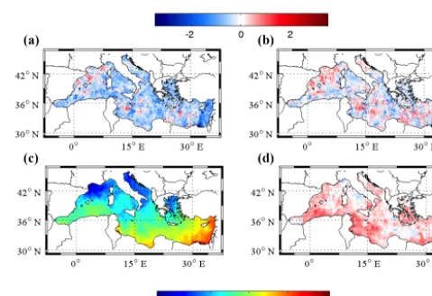
Figure 2. MMSE estimates for the first day of the test period (25 April 2008) using a training period of 15 days, S1-SST (top panel, left) and the corresponding estimate for S2-SST (top panel, right), SST from satellite (bottom panel, left) and best ensemble member SST (bottom panel, right).
The different statistical regression algorithms are summa-rized in Table 3. A flow chart (Fig. 1) is provided to help the reader in understanding the logical path that authors de-signed for the described procedures.
5 MMSE experiments
Table 3.Nomenclature and characteristics of the four MMSE algorithms used.
MMSE methods Extended name Main characteristics
S1 Classical SE Krishnamurti et al. (1999) regression
S2 Classical SE modified Seasonal signal removal before the regression
S3 Spatially filtered SE Seasonal signal removal before the regression and spatial filter
applied to the regression estimate
S4 EOF-based SE EOFs evaluated from observations and members and regression
performed on the EOF coefficients.
Figure 3. MMSE estimates for the last day of test period (4 May 2008), S1-SST (top panel, left) and the corresponding es-timate for S2-SST (top panel, right), SST from satellite (bottom panel, left) and best ensemble member SST(bottom panel, right).
5.1 Classical SE method experiments
In order to find the minimum training period length possi-ble, a simple experiment has been done using the observa-tions as one of the ensemble members in the training pe-riod. This test can be considered as the maximum skill that could be achieved with a MMSE approach, and it is also a way to check the coefficient estimates. For a training period of 15 days, all the regression coefficients are 0 except for the weight related to the observational member, which is re-trieved to be 1. Trimming the data set (removing members), we noticed that when the training period days (M) are less than the number of ensemble members involved (N), in our case 9 (Table 1), the algorithm fails, giving incorrect values for the coefficients. Hence the minimum training period units must be such that M > N. In our case any training period longer than 10 days will work well. However to add robust-ness to regression algorithm, we set 15 days as the minimum length of the learning period. On the basis of a 15-day train-ing period, Fig. 2 shows the S1 and S2 posterior estimates for the first day of the test analysis period. S1 and S2 recon-structed SST fields are very noisy compared to observations, and both S1 and S2 are clearly worse than the BEM estimate.
The two estimates at the end of the test analysis period are shown in Fig. 3, where the overfitting problem is even more evident. The field noise can be reduced by lengthen-ing the trainlengthen-ing period to 35 days, as shown in Figs. 4 and 5. Both S1 and S2 predictions show a reduction in the warm bias with respect to the BEM in the eastern Mediterranean (Figs. 2 and 3). However S1 does not show any improvement in terms of RMSE and ACC (data not shown). Even if we ne-glected the overfitting that affects SE prediction trained with a learning period longer than 35 days, we think long train-ing is out of the scope of our research since we are focused on a potential operative approach In order to examine the ef-fect of the specific MMSE members on the S1 estimation performance, we create three different MMSE data sets (Ta-ble 4). Data set A corresponds to an overconfident (Weigel et al., 2008) data set or correlated ensemble members. We consider data set B, which is well dispersed, to be the best and the worst ensemble member, together with other corre-lated members, i.e. with similar RMSE, SD and ACC (see Table 4), while data set C, which is poorly dispersed, con-siders worst members together with correlated members. To quantify the differences between the three data sets, a bias in-dicatord is estimated. This value corresponds to the domain averaged SST difference as follows:
d= hFt(x, y)−Ot(x, y)
Ot(x, y)
,i (11)
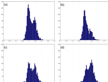
where the triangular parentheses indicate the domain aver-age. Ifdis close to 0, this means a small data set bias, while a positive (negative)d means a positive (negative) SST bias. Figure 6 shows the distributions of d for different MMSE data sets. The distributions are bimodal with two maxima, the first around 0◦C and the second around 0.05◦C, which means that the data set statistically tends to overestimate the spatial mean SST. From these distributions we can also ob-serve that
– data set A has the smallest bias because thed=0◦C peak is larger than the peak at 0.05◦C;
Figure 4. MMSE estimates for the first day of the test period (25 April 2008) using a training period of 35 days, S1-SST (left panel) and the corresponding estimate for S2-SST (right panel).
Figure 5.MMSE estimates with a 35-day training period and for the last day of the test period (4 May 2008), S1-SST (left panel) and the corresponding estimate for S2-SST(right panel).
– for data set C, which is constructed from badly dis-persed model ensemble members, the estimate enhances the positive bias.
Figure 7 presents the histogram ofd for the S1 estimates on the first day of analysis for the whole of 2008 as a function of the full and subsampled MMSE data sets. It is evident that all the MMSE data sets give a S1 distribution peak around d=0◦C with a strong reduction in the distribution width.
This means that the algorithm is capable of neglecting the in-formation from biased members. The small S1 bias remains the same till the 5th day of the analysis period (not shown), after which the performance of the algorithm starts to deteri-orate. On the last day, there is a nearly flat histogram (Fig. 8). This means that unbiased analyses can be produced for up to 5 days with a 15-day training period, no matter which MMSE data set is used. With respect to RMSE, different MMSE data sets and training period lengths give different results already on day 1 of the analysis period, as shown in Table 5, both for S1 and S2 posterior analysis estimates. It is now evident that the overconfident data set and the longest training pe-riod (35 days) produce on average the lowest RMSE values during the analysis period. In conclusion, the Krishnamurti et al. (1999) method can be applied relatively successfully to the oceanic multi-model state estimation case, using at least a 14 (and up to 35)-day training period and with only a five-member ensemble data set if the quality of the chosen members is high. However, the S1 and S2 estimates are both affected by noise, and only a modification in the regression method will lead to a low-RMSE posterior-analysis noise-less estimate. We want to enhance that these performances are due to the usage of a multi-model multi-physics choice.
Table 4.MMSE data sets: members are detailed in Table 1.
MMSE data set A MMSE data set B MMSE data set C (Overconfident data set) (Well-dispersed data set) (Badly dispersed data set)
INGV-SYS3a2 INGV-SYS3a2 Mercator-V1
INGV-SYS4a3 HCMR HCMR
Mercator-V0 INGV MP1 INGV MP1
Mercator-V1 INGV MP2 INGV MP2
HCMR INGV MP3 INGV MP3
INGV MP1 INGV MP4 INGV MP4
Table 5.RMSE mean value throughout the analysis period for the full data set (see Table 1) and the three data sets of Table 4 as a function of the training period length and S1 and S2.
SE members
Training periods
15 days 25 days 35 days
S1 S2 S1 S2 S1 S2
Full 1.99 1.59 1.07 0.86 0.79 0.68
Data set A 1.19 0.96 0.77 0.65 0.62 0.56
Data set B 1.21 0.98 0.81 0.67 0.64 0.57
Data set C 1.30 1.05 0.86 0.71 0.68 0.59
Here for the first time we can assess the SE prediction impact in terms of the data set composition. Our research activity be-gins studying the characteristic that a data set should fulfill in terms of the spread of the ensemble and the mean bias of each member. Only a multi-model multi-physics data set could satisfy all the requirements. We can prove this inference with a set of two subsamples: subsample D: multi-model (MM): INGV-SYS3a2, INGV-SYS4a3, Mercator-V0, Mercator-V1 and HCMR; subsample E: multi-model multi-physics (MM-MP): INGV-SYS3a2, INGV-SYS4a3, Mercator-V1, HCMR and INGV MP1. From Fig. 9 one can clearly see the improve-ments to SE brought about by substituting one member with a simulation with similar performances.
5.2 New SE method experiments
Figure 6.Distributions ofdin Eq.(11) for the full data set(a), overconfident data set A(b), well-dispersed data set B(c)and badly dispersed
data set C(d). The bin width is 0.05◦C. Area under the curve equals the total number of models per day in the year 2008.
Figure 7.The effect of multi-model composition in the distributions ofdfor the full data set(a), overconfident data set A(b), well-dispersed
data set B(c)and badly dispersed data set C(d). The bin width is 0.05◦C. The effect of multi-model combination of proposed subsamples
Figure 8.The effect of multi-model composition on the distributions ofdfor the full data set(a), overconfident data set A(b), well-dispersed
data set B(c)and badly dispersed data set C(d). The bin width is 0.05◦C. The effect of multi-model combination of proposed subsample on
the SE estimates valid for 10th (last) day of the test period with a training period of 14 days.
Figure 9.Domain average (over the Mediterranean) and time mean the over year 2008 of the RMSE for a 15-day training period for the overconfident data set A.
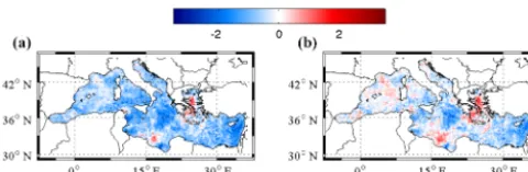
is 164 obtained with 35 days. As expected, the number of EOFs retained increases when we extend the training pe-riod, with some variability during the year. Usually the mini-mum number of EOFs was found in the summer. The S3 and S4 posterior estimates are shown in Figs. 12 and 13 for the first day of the test analysis period. Both estimates are much smoother than the equivalent S1 and S2 estimates in Fig. 2. The S3 also seems to be less biased with respect to obser-vations. A map of the differences between the truth and the SE estimates highlights the better performances of S3 com-pared to S4 for the whole test analysis period (not shown).
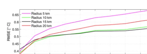
Figure 10. Domain average (over the Mediterranean) and time mean over the year 2008 of the RMSE of S3 estimates training the overconfident data set A for 15 days and with a different circular radius.
14 16 18 20 22 24 26 28 30 32 34 36 0
50 100 150 200
Length of the training period [days]
Number of EOFs
February March April May June July August September October November
Figure 11.Number of retained EOFs histogram, on ordinates the length of the training period, colour bar proportioned to the day of the experiments.
Figure 12. S3 and S4 estimate for the first day of the test period (25 April 2008) using a training period of 15 days, SE3-SST (left
panel,a) and the corresponding estimate for S4-SST (right panel,
b).
Figure 13.S3 and S4 estimates valid the last day of the test period (4 May 2008) using a training period of 15 days, S3-SST (left panel,
a) and the corresponding estimate for S4-SST (right panel,b).
1 2 3 4 5 6 7 8 9 10
0.5 1 1.5 2
Analysis period
R
M
S
E
°
C
S1 S2 S3 S4 B.E.M.
Figure 14. Domain average (over the Mediterranean) and time mean during the year 2008 of SE prediction RMSE overconfident data set A. SE predictions trained for 15 days. Error bars stand for the standard deviation of the RMSE during the year.
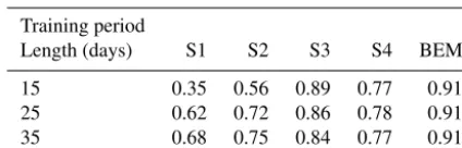
super-ensemble estimate. ACC mean values are listed in Ta-ble 6 and are also depicted in Fig. 15. As a result of this skill, S3 decreased its consistency in relation to an increase of the length of the training period. On the other hand, S4
1 2 3 4 5 6 7 8 9 10
0 0.2 0.4 0.6 0.8 1
Analysisperiod
ACC S1S2
S3 S4 B.E.M.
Figure 15.Spatial average over the Mediterranean Sea and time mean during 2008 SE prediction ACC of overconfident data set A. SE predictions trained for 15 days.
1 2 3 4 5 6 7 8 9 10
−0.2 0 0.2
Analysis period
BIAS
°
C
S1 S2 S3 S4 B.E.M.
Figure 16.Spatial average over the Mediterranean Sea and time mean during 2008 SE prediction bias of overconfident data set A. SE predictions trained for 15 days. Error bars stand for the standard deviation of the bias during the year.
had a constant ACC irrespective of the chosen training pe-riod. However BEM was the most “consistent” member. This means that, although our SE can be used as a statistical tool, physical constraints are needed in order to have more con-sistent maps too. Nevertheless it should be highlighted that S1 and S2 are even less consistent compared to the worst-contributing member. Bias skills were also evaluated for the proposed methodologies; however, as expected due to their construction, all the SE estimates were unbiased (Fig. 16). Thus no inference can be drawn from the bias skills.
6 Conclusions
Table 6.ACC mean value throughout the analysis period for data set A (see Table 1) as a function of the training period length for the proposed SE methodologies.
Training period
Length (days) S1 S2 S3 S4 BEM
15 0.35 0.56 0.89 0.77 0.91
25 0.62 0.72 0.86 0.78 0.91
35 0.68 0.75 0.84 0.77 0.91
cannot be successfully applied to estimate oceanic MMSE SST. An initial improvement to S1, named S2, is the subtrac-tion of the seasonal signal in the ensemble members and the unbiased estimator. This leads to a strong reduction in RMSE (more than 20 %), but the resulting field is noisy compared to observations. This is the well-known overfitting problem of the technique described in Kharin and Zwiers (2002). The further modification of S2 using a simple spatial filter, named S3, can give lower RMSE values than the BEM for the entire 10-day analysis period. A new methodology, based on EOFs, named S4, also reduces the RMSE. However S3 outperforms S4 and could represent a practical technique for applications in operational oceanographic analyses for up to 10 days on the basis of the previous 15 days of analyses. One could won-der if the proposed combination of models can offer interest-ing skill below the sea surface as well. Unfortunately sparse-ness of subsurface observations make it very hard to envis-age a horizontal EOF method that allow us to correctly take advantage of and spread the information coming from the observation itself. We must remark that this is only a starting point. MMSE techniques for ocean state estimation problems require further study before optimal methods can be found. In this paper we show that with a rather limited but over-confident data set (with a low bias of the starting ensemble members) the RMSE analysis can be improved. This poste-rior value-added estimation could, for example, be used to produce a more accurate MMSE analysis data set.
Future developments could involve the addition of phys-ical constraints during the regression, considering for ex-ample cross correlations with atmospheric forcing. MMSE should also be applied to the ocean forecast problem instead of the analysis problem. The difference for MMSE forecast estimates is that atmospheric forecast uncertainties are not contained in training period analyses, and the size of the ensemble members required could increase considerably, as well as the complexity of the estimation problem.
Data availability
Appendix A: Data set description
The analysis systems that generated the ensemble members of the experiments used in this paper are briefly described below:
– SYS3a2: system composed of the numerical code of OPA8.2 implemented in the Mediterranean Sea (Tonani et al., 2008) and 3DVAR assimilation scheme (Dobricic and Pinardi, 2008).
– SYS4a3 uses NEMO 2.3 (Oddo et al., 2009) as a numer-ical model and also 3DVAR for the assimilation. Other differences are due to the different boundary conditions, since here the model is nested within the monthly mean climatological field computed from the daily output of the Mercator 14oresolution global model.
– Mercator-V0 (PSY2V3R1): the numerical code is based on NEMO 1.09, and it is implemented in the North At-lantic and Mediterranean Sea with a horizontal resolu-tion of 121oand 50 vertical levels. The real-time system from 2008 to 2010 was initialized for a calibration phase in 2006. ECMWF analysis and forecasts are coupled daily. The data assimilation scheme is based on a local singular evolutive extended Kalman filter (Pham et al., 1998), and the observation assimilated are in situ tem-perature and salinity profiles in the Coriolis database, together with SST and along-track SLA. Further details are described in Brasseur et al. (2005).
– Mercator-V1(PSY2V4R1): the numerical code is based on NEMO 3.1 version, and it is implemented in the North Atlantic and Mediterranean Sea with a horizon-tal resolution of 121o and 50 vertical levels. The real-time system was initialized in October 2006 from a 3-D climatology of temperature and salinity (Levitus et al., 2005) providing analysis and forecast from 2010 to 2013. The code includes several improvements in the model configuration such as open-boundary condition (from the global system) and higher-frequency atmo-spheric forcing (each 3 h). The data assimilation scheme is similar to the previous version plus a bias correction based on the 3DVAR assimilation scheme (Lellouche et al., 2013)
– HCMR: Hellenic Centre for Marine Research (Korres et al., 2009). The Mediterranean Sea model is based on the Princeton Ocean Model (POM) code, a primi-tive equations 3-D model using the Mellor–Yamada 2.5 turbulence closure scheme. The model has a bottom-following vertical sigma coordinate system, a free sur-face and a split-mode time step. Potential tempera-ture, salinity, velocity and surface elevation are prog-nostic variables. The model has a horizontal resolution of 101o and 25 sigma layers along the vertical with a
logarithmic distribution near the surface and the bot-tom. The model includes parameterization of the main Mediterranean rivers, while the inflow/outflow at the Dardanelles is treated with open-boundary techniques. The Mediterranean model is forced with hourly surface fluxes of momentum, heat and water provided by the POSEIDON–ETA high-resolution (201o) regional atmo-spheric model (Papadopoulos and Katsafados, 2009) is-suing forecasts for 5 days ahead. The assimilation sys-tem for the Mediterranean Sea hydrodynamic model is very similar to the one presented in the work of Korres et al. (2010). It is based on the singular evolutive ex-tended Kalman (SEEK) filter with covariance localiza-tion and partial evolulocaliza-tion of the correclocaliza-tion direclocaliza-tions. The error covariance matrix is approximated with 60 EOF modes (correction directions), where the first 18 (the most dominant ones) are evolved with the model dynamics while the rest are kept invariant in time. The localization technique adopted for the Mediterranean Sea forecasting system is explained in Korres et al. (2010). The method localizes the covariance matrix by neglecting observations beyond a cut-off radius which is selected upon sensitivity studies to be equal to 200 km. – NEMO multi-physics: this is the same as SYS4a3
NEMO 2.3 code without assimilation but with different model physical parameterizations.
Appendix B: Algorithm time averages and projection on EOFs
Here we show how the observed and model fields are de-composed into different temporal signals. Let us consider O(x, y, t )to be the daily OI-SST andF (x, y, t )one of the model members’ daily mean SST. We can always decom-pose the signal into seasonal mean, training period mean and anomaly. Considering the two time average operators:
hf (x, y)is =1
q
q X
t=1
f (x, y, t )) (B1)
hf (x, y)iTR= 1
N
N X
t=1
f (x, y, t )) , (B2)
where “q” is the number of days in the month of the year with a value evaluated over a long time series mean from 2001 to 2007, andN is the number of training days, we write O (x, y, t )= hO (x, y)iS+ hO (x, y)iTR+O0(x, y, t ) ,
Author contributions. Jenny Pistoia with the supervision of Paolo Oddo and Nadia Pinardi designed and performed all the INGV multi-physics simulations and collected all the INGV anal-ysis. Matthew Collins supervised all the activity connected with the SE based on EOFs. Gerasimos Korres and Yann Drillet pro-vide respectively the HCMR and Mercator analysis members in the same grid of INGV members in order to build the MMSE data set. Jenny Pistoia prepared the manuscript with contributions from all co-authors.
Acknowledgements. This work was supported by the University
of Bologna as part of the graduate programme in geophysics and by the MyOcean2 Project. The CMCC Gemina project funded J. Pistoia’s studies at the University of Exeter. Publication was supported from the Italian Ministry of Education, University and Research under the project RITMARE.
Edited by: R. Archetti
Reviewed by: M. Bostenaru-Dan and one anonymous referee
References
Boria, R. A., Olson, L. E., Goodman, S. M., and Anderson, R. P.: Spatial filtering to reduce sampling bias can improve the per-formance of ecological niche models, Ecol. Model., 275, 73–77, doi:10.1016/j.ecolmodel.2013.12.012, 2014.
Brasseur, P., Bahurel, P., Bertino, L., Birol, F., Brankart, J.-M., Ferry, N., Losa, S., Remy, E., Schröter, J., Skachko, S., Testut, C.-E., Tranchant, B., Van Leeuwen, P. J., and Ver-ron, J.: Data assimilation for marine monitoring and predic-tion: The MERCATOR operational assimilation systems and the MERSEA developments, Q. J. Roy. Meteor. Soc., 131, 3561– 3582, doi:10.1256/qj.05.142, 2005.
Casey, K., Brandon, T., Cornillon, P., and Evans, R.: The Past, Present and Future of the AVHRR Pathfinder SST Program, Oceanography from Space: Revisited, 2010.
Dobricic, S. and Pinardi, N.: An oceanographic three-dimensional variational data assimilation scheme, Ocean Model., 22, 89–105, doi:10.1016/j.ocemod.2008.01.004, 2008.
Evans, R., Harrison, M., Graham, R., and Mylne, K.: Joint Medium-Range Ensembles from The Met. Office and ECMWF Sys-tems, Mon. Weather Rev., 128, 3104–3127, doi:10.1175/1520-0493(2000)128<3104:JMREFT>2.0.CO;2, 2000.
Feddersen, H., Navarra, A., and Ward, M.: Reduction of model sys-tematic error by statistical correction for dynamical seasonal pre-dictions, J. Climate, 12, 1974–1989, 1999.
Gaspar, P., Grégoris, Y., and Lefevre, J.: A simple eddy kinetic en-ergy model for simulations of the oceanic vertical mixing: Tests at Station Papa and long-term upper ocean study site, J. Geophys. Res., 95, 176–193, doi:10.1029/JC095iC09p16179, 1990. INGV: Istituto Nazionale Geofisica e Vulcanologia,
Multi-Model Multi-Physics Dataset, available at: http://oceanop.bo. ingv.it/mmse-dataset, Operational Oceanography Group (http: //oceanop.bo.ingv.it/), 2015.
Kalnay, E. and Ham, M.: Forecasting forecast skill in the Southern Hemisphere, American Meteorological Society, preprints of the
3rd International Conference on Southern Hemisphere Meteorol-ogy and Oceanography, Buenos Aires, 13–17 November, 24–27, 1989.
Kharin, V. and Zwiers, F.: Climate predictions with multimodel en-sembles, J. Climate, 15, 793–799, 2002.
Korres, G., Nittis, K., Hoteit, I., and Triantafyllou, G.: A high resolution data assimilation system for the Aegean
Sea hydrodynamics, J. Marine Syst., 77, 325–340,
doi:10.1016/j.jmarsys.2007.12.014, 2009.
Korres, G., Nittis, K., Perivoliotis, Tsiaras, Papadopoulos, , and Tri-antafyllou, H. G.: Forecasting the Aegean Sea hydrodynamics within the POSEIDON-II operational system, Journal of Opera-tional Oceanography, 3, 37–49, 2010.
Krishnamurti, T., Kishtawal, C., LaRow, T., Bachiochi, D., Zhang, Z., Williford, C., Gadgil, S., and Surendran, S.: Improved Weather and Seasonal Climate Forecasts from Multimodel Su-perensemble, Science, 285, 1548–1550, 1999.
Krishnamurti, T., Kishtawal, C., Zhang, Z., LaRow, T., Ba-chiochi, D., Williford, E., Gadgil, S., and Surendran, S.: Multimodel Ensemble Forecasts for Weather and Seasonal
Climate, J. Climate, 13, 4196–4216,
doi:10.1175/1520-0442(2000)013<4196:MEFFWA>2.0.CO;2, 2000.
Lellouche, J.-M., Le Galloudec, O., Drévillon, M., Régnier, C., Greiner, E., Garric, G., Ferry, N., Desportes, C., Testut, C.-E., Bricaud, C., Bourdallé-Badie, R., Tranchant, B., Benkiran, M., Drillet, Y., Daudin, A., and De Nicola, C.: Evaluation of global monitoring and forecasting systems at Mercator Océan, Ocean Sci., 9, 57–81, doi:10.5194/os-9-57-2013, 2013.
Lenartz, F., Mourre, B., Barth, A., Beckers, J., Vandenbulcke, L., and Rixen, M.: Enhanced ocean temperature forecast skills through 3-D super-ensemble multi-model fusion, Geophys. Res. Lett., 37, L19606, doi:10.1029/2010GL044591, 2010.
Levitus, S., Antonov, J., and Boyer, T.: Warming of the world ocean, 1955–2003, Geophys. Res. Lett., 32, L02604, doi:10.1029/2004GL021592, 2005.
Lorenz, E. N.: Deterministic Nonperiodic Flow,
J. Atmos. Sci., 20, 130–141,
doi:10.1175/1520-0469(1963)020%3C0130:DNF%3E2.0.CO;2, 1963.
Madec, G.: NEMO ocean engine, Note du Pôle de modélisation, In-stitut Pierre-Simon Laplace (IPSL), France, No. 27 ISSN: 1288-1619, 2008.
Madec, G., Delecluse, P., Imbard, M., and Levy, C.: OPA version 8.1 ocean general circulation model reference manual, Technical Report, LODYC/IPSL, Note 11, Paris, France, 91 pp., 1998. Marullo, S., Buongiorno Nardelli, B., Guarracino, M., and
Santo-leri, R.: Observing the Mediterranean Sea from space: 21 years of Pathfinder-AVHRR sea surface temperatures (1985 to 2005): re-analysis and validation, Ocean Sci., 3, 299–310, doi:10.5194/os-3-299-2007, 2007.
Mellor, G. and Yamada, T.: Development of a turbulence closure model for geophysical fluid problems, Rev. Geophys. Space Ge., 20, 851–875, 1982.
Mellor, G. L. and Blumberg, A. F.: Modeling Vertical and Horizontal Diffusivities with the Sigma Coordinate System, Month. Weather Rev., 113, 1379–1383, doi:10.1175/1520-0493(1985)113<1379:MVAHDW>2.0.CO;2, 1985.
Oddo, P., Adani, M., Pinardi, N., Fratianni, C., Tonani, M., and Pet-tenuzzo, D.: A nested Atlantic-Mediterranean Sea general circu-lation model for operational forecasting, Ocean Sci., 5, 461–473, doi:10.5194/os-5-461-2009, 2009.
Pacanowski, R. C. and Philander, S. G. H.: Parameterization of Ver-tical Mixing in Numerical Models of Tropical Oceans, Journal of Physical Oceanography, 11, 1443–1451, doi:10.1175/1520-0485(1981)011<1443:POVMIN>2.0.CO;2, 1981.
Papadopoulos, A. and Katsafados, P.: Verification of operational weather forecasts from the POSEIDON system across the East-ern Mediterranean, Nat. Hazards Earth Syst. Sci., 9, 1299–1306, doi:10.5194/nhess-9-1299-2009, 2009.
Pavan, V. and Doblas-Reyes: Multi-model seasonal hindcasts over the Euro-Atlantic: skill scores and dynamic features, Climate Dynamics, 16, 611–625, available at: http://link.springer.com/ article/10.1007/s003820000063, 2000.
Pham, D., Verron, J., and Roubaud, M.: A singular evolutive ex-tended Kalman filter for data assimilation in oceanography, J. Marine Syst., 16, 323–340, 1998.
Pinardi, N. and Masetti, E.: Variability of the large scale general cir-culation of the Mediterranean Sea from observations and mod-elling: a review, Palaeogeography, Palaeoclimatology, Palaeoe-cology, 158, 153–173, doi:10.1016/S0031-0182(00)00048-1, 2000.
Pinardi, N., Bonazzi, A., Dobricic, S., Milliff, R., Wikle, C., and Berliner, L.: Ocean ensemble forecasting. Part II: Mediterranean Forecast System response, Q. J. Roy. Meteor. Soc., 137, 657, doi:10.1002/qj.816, 2011.
Rixen, M., Ferreira-Coelho, E., and Signell, R.: Surface drift prediction in the Adriatic Sea using hyper-ensemble statis-tics on atmospheric, ocean and wave models: Uncertainties and probability distribution areas, J. Marine Syst., 69, 86–98, doi:10.1016/j.jmarsys.2007.02.015, 2008.
Rixen, M., Book, J. W., Carta, A., Grandi, V., Gualdesi, L., Stoner, R., Ranelli, P., Cavanna, A., Zanasca, P., Baldasserini, G., Trangeled, A., Lewis, C., Trees, C., Grasso, R., Giannechini, S., Fabiani, A., Merani, D., Berni, A., Leonard, M., Martin, P., Row-ley, C., Hulbert, M., Quaid, A., Goode, W., Preller, R., Pinardi, N., Oddo, P., Guarnieri, A., Chiggiato, J., Carniel, S., Russo, A., Tudor, M., Lenartz, F., and Vandenbulcke, L.: Improved ocean prediction skill and reduced uncertainty in the coastal region from multi-model super-ensembles, J. Marine Syst., 78, Supple-ment, S282–S289, doi:10.1016/j.jmarsys.2009.01.014, 2009. Robinson, A. R., Hecht, A., Pinardi, N., Bishop, J., Leslie, W. G.,
Rosentroub, Z., Mariano, A. J., and Brenner, S.: Small syn-optic/mesoscale eddies and energetic variability of the eastern Levantine basin, Nature, 327, 131–134, doi:10.1038/327131a0, 1987.
Shukla, J., Marx, L., Paolino, D., Straus, D., Anderson, J., Ploshay, J., Baumhefner, D., Tribbia, J., Brankovic, C., Palmer, T., Chang, Y., Schubert, S., Suarez, M., and Kalnay, E.: Dynami-cal Seasonal Prediction, B. Am. Meteorol. Soc., 81, 2593–2606, doi:10.1175/1520-0477(2000)081<2593:DSP>2.3.CO;2, 2000. Stefanova, L. and Krishnamurti, T.: Interpretation of
Sea-sonal Climate Forecast Using Brier Skill Score, The
Florida State University Superensemble, and the
AMIP-I Dataset, J. Climate, 15, 537–544,
doi:10.1175/1520-0442(2002)015<0537:IOSCFU>2.0.CO;2, 2002.
Stensrud, D. J., Bao, J.-W., and Warner, T. T.: Using Ini-tial Condition and Model Physics Perturbations in Short-Range Ensemble Simulations of Mesoscale Convective Sys-tems, Mon. Weather Rev., 128, 2077–2107, doi:10.1175/1520-0493(2000)128<2077:UICAMP>2.0.CO;2, 2000.
Stephenson, D. B. and Doblas-Reyes, F. J.: Statistical methods for interpreting Monte Carlo ensemble forecasts, Tellus A, 52, 300– 322, doi:10.1034/j.1600-0870.2000.d01-5.x, 2000.
Tonani, M., Pinardi, N., Fratianni, C., Pistoia, J., Dobricic, S., Pensieri, S., de Alfonso, M., and Nittis, K.: Mediterranean Forecasting System: forecast and analysis assessment through skill scores, Ocean Sci., 5, 649–660, doi:10.5194/os-5-649-2009, 2009.
Toth, Z. and Kalnay, E.: Ensemble Forecasting at NCEP and the Breeding Method, Mon. Weather Rev., 125, 3297–3319, doi:10.1175/1520-0493(1997)125<3297:EFANAT»2.0.CO;2, 1997.
Vandenbulcke, L., Beckers, J.-M., Lenartz, F., Barth, A., Poulain, P.-M., Aidonidis, M., Meyrat, J., Ardhuin, F., Tonani, M., Fra-tianni, C., Torrisi, L., Pallela, D., Chiggiato, J., Tudor, M., Book, J., Martin, P., Peggion, G., and Rixen, M.: Super-ensemble tech-niques: Application to surface drift prediction, Prog. Oceanogr., 82, 149–167, doi:10.1016/j.pocean.2009.06.002, 2009.
von Storch, H. and Navarra, A.: Spatial Patterns: EOFs and CCA. In Analysis of Climate Variability: Application of Statistical Tech-niques, Springer Verlag, Berlin, 227–257, ISBN-13: 978-3-642-08560-4, 1995.
Weigel, A. P., Liniger, M. A., and Appenzeller, C.: Can multi-model combination really enhance the prediction skill of probabilis-tic ensemble forecasts?, Q. J. Roy. Meteor. Soc., 134, 241–260, doi:10.1002/qj.210, 2008.