Hyperspectral Nonlinear Unmixing: Endmember
extracting Using Iterative Simplex CNN Method
Nandhini .K, Porkodi .R
Abstract— Hyperspectral remote sensing images are showing rapid improvements in many domain such as weather, land cover classification, underwater species identification, exploring the space etc. Over the past decades pixel-wise classification have been focussed by the research community by improving accuracy, but still the problems persists due to low spatial resolution and multiple scattering effects of light generates the mixed substances in a pixel. In recent decade, the sub-pixel-wise and object based methods are focussed in a hyperspectral image classification. This paper concentrates on the experimentation of hyperspectral sub-pixel wise classification. There are two different types of spectral unmixing techniques are based on linear and nonlinear unmixing approaches. In linear unmixing techniques assumes that in macroscopic pixel level, pure substances may present per pixel, but in reality the intimate mixtures present in microscopic level due to the scattering effects of light. Basically there are two step involved in the nonlinear unmixing: endmembers extraction and abundances fractions present per pixel. This paper proposed the novel iterative simplex volume analysis Convolutional Neural Network (IS_CNN) method to extract the end members. And further, this research work employed fully constrained least square (FCLS) method to extract the endmembers of the hyperspectral data. The overall performance of the proposed method is measured with Root mean squared error (RMSE), the IS_CNN RMSE Average value for all extracted end members is 0.08 which shows the significant performance when compared with the FCLS method.
Index Terms—CNN Method, Hyperspectral data, Nonlinear unmixing, Simplex Volume Analysis
—————————— ——————————
1 I
NTRODUCTIONImaging spectrometer often records the continuous spectral information of the particular scene which is present in the huge dimensionality of narrow adjacent bands (hyperspectral (HS) bands). Identifying and classifying the pure substances are playing a major role in any hyperspectral remote sensing domains. Basically, the remote sensing image classifications are fall into three broad categories: 1) Pixel-wise classification, 2) Sub-pixel-wise classification, and 3) Object-based classification methods. In general, the particular scene contains only one type of pure substances presented per pixel is called homogeneity spatial area. If there are two or more substances presented per pixel are referred to as heterogeneity spatial area. The pixel-wise classification is a traditional way of classifying the class labels by assuming that the pixels present in the bands are pure pixels. There are three different approaches are widely used for pixel-wise classification methods are: Supervised, unsupervised, and semi-supervised learning. The pixel-wise methods are highly recommended for homogeneity spatial area, but in heterogeneity spatial area, there is a pitfall in assuming that the particular scene contains only pure pixels are often leads to the low accuracy. Sub-pixel-wise classification methods are suitable for heterogeneity spatial area. Here, in each mixed pixel the pure substances are identified and classified. The performance in the accuracy is very high when compared to the pixel-wise-classification, especially in the heterogenic spatial area. The object-based
classification method is a different concept where the geographical objects are considered as the objects instead of the pixel values. Initially, image segmentation will be carried out and object-based approaches like ArcGIS feature analyst, E-cognition etc. are used to retrieve the spatial, textural, and contextual information [1] [2].
The mixture of substances in a pixel is referred to as spectral mixing which is classified by sub-pixel-wise classification techniques. There are two basic steps involved in the spectral unmixing 1) endmember determination and 2) abundance estimation. The presence of pure substances in each mixed pixel is determined as endmembers. The corresponding endmember’s fractions per pixel are estimated as abundance. There are two different approaches are used widely for spectral unmixing, they are linear and nonlinear unmixing. Assuming that the incident radiation will interact with only one substance by eliminating the multiple scattering between the substances are referred to as linearly mix per pixel in the macroscopic scale which requires linear unmixing approaches. If more than one substances are intimately present per pixel are referred to as nonlinear mixing in microscopic scale level which requires nonlinear unmixing approaches [3] [4] [5]. Figure 1 shows the different stages in the spectral unmixing [1].
The stages of spectral unmixing are the following; first stage is to reduce the hyperspectral dimensionality from high to low. The next stages are to extract the endmembers in a pixel and estimate the abundance fractions present in each pixel. In general the nonlinear function for spectral unmixing can be expressed in equation (1):
𝑌 = 𝑓(Μ, 𝑥) + 𝑛 … … … …. (1)
Here f is a nonlinear function, where M denotes the endmembers: {m1, m2, m3… mk}, and x is a transposed vector
with additive noise n [6]. The dimensionality reduction in
————————————————
Nandhini K, Department of Computer Science, Bharathiar University, Coimbatore-641046, India. E-mail: [email protected]
79
hyperspectral unmixing plays a crucial role in reducing the time and space complexity in computation. Initially, the HS data are projected into low dimensionality followed by using endmember determination algorithm where the pure substances are determined and then abundances are estimated. This paper concentrates and proposed the novel algorithm for nonlinear unmixing by considering the real world scenario.
Figure 1 The Stages in Spectral Unmixing
The remaining of the sections is organized as follows: Section 2 discusses about the literature study and analysis of nonlinear unmixing. Section 3 describes the methodology framework and implementation of the novel proposed algorithm. Section 4 discusses about the experimental results and section 5 concludes the research study with future work.
2 INFERENCE ON NONLINEAR UNMIXING METHODS
The widely used hyperspectral sensors dataset by a research community are AVIRIS, HYDICE, AISA, APEX, CASI, HyMap, OMEGA etc. These sensors collect the information by the number of bands, the range of the spectral (µm) and instantaneous field of view IFOV (m). Due to the scattering effects with the sensor there will be distinct substances intimate in a same microscopic pixel referred to as nonlinear mixing. There are different types of approaches and techniques are widely used for nonlinear unmixing are the following: intimate mineral mixture models, radiosity based approaches, neural networks, kernel methods, bilinear models, ray tracing, support vector machine techniques, piecewise linear techniques, manifold learning techniques, and nonlinear mixing detection [7]. The intimate mixtures in a pixel need to be concentrated by considering the spatial objects to improve the nonlinear unmixing algorithms. In modified bilinear model (MBM), the virtual endmembers andabundance mapping are subject to the sum-to-one constraint. The quadratic programming approaches are included on distinct parameters in MBM. The above method is compared by spatial information for nonlinear spectral mixture analysis (SNSMA) method considered the spatial objects by adopting the local windows in a pre-classification mapping. The above methods are experimented in HYDICE Urban hyperspectral dataset. SNSMA proves to best when compared with the following methods LS, FCLS, EVLMM, SLS, SFCLS, and NSMA [8].
Endmembers are determined by many linear and nonlinear methods which may parametric or non-parametric techniques. The simplex growing algorithm (SGA) was enhanced by new SGA (NSGA) and kernel NSGA (KNSGA) to determine the endmembers by faster implementation. Liaoying Zhao et.al (2015) focuses on the performance computing and they experimented with generated synthetic dataset with USGS spectral library and AVIRIS Cuprite hyperspectral real time dataset [9]. Abderrahim Halimi et al proposed a Metropolis-within-Gibbs algorithm in Bayesian algorithm to avoid the complexity in obtaining the analytical expressions of Bayesian estimators. Linear and nonlinear mixing approaches are experimented in AVIRIS Moffett Filed. Generalized Bilinear Model (GBM) is used for macroscopic components mixture and VCA algorithm is frequently used to determine the endmembers for Moffett field. A hierarchical Bayesian method is employed for nonlinearity with the intimate mixtures in a pixel [10]. Adopting the spatial relations between the adjacent pixels of the HS data in Bayesian algorithm attain the spectral information by focussing on the spectral unmixing [11].
The matched filtering (MF), mixture tune matched filtering (MTMF), and constrain energy minimization (CEM) are subpixel unmixing algorithms which is experimented with the EO-1 Hyperion Yoann Altmann et.al considers that the proposed model of nonlinear unmixing algorithm assumes that the pixel reflectances of unidentified pure substances are contaminated by additive white Gaussian noise which requires a second-order polynomial functions. The Bayesian algorithm is proposed with the Hamiltonian Monte Carlo algorithm due to large number of estimated Bayesian parameters. These algorithm performances are experimented with the synthetic datasets and the real time Hyspex Madonna dataset [12]. The kernel based nonlinear unmixing is from the Hilbert Space vector valued functions which got enhanced by dependant bands and using the contributions of the nonlinear neighbours. The kernel valued nonlinear functions are jointly modelled with the matrix valued kernels with the extensive range of the nonlinearities. The alternative direction method of multipliers (ADMM) is applied in the proposed iterative algorithm. FCLS, the scalar RKHS model (khype), and Extended endmember matrix method (Ext) are employed and analyzed the performance with the proposed kernel method. It is experimented with synthetic datasets and Meris Spectrometer Gulf of Lion, France HS data [13]. The extreme learning machine (ELM) regression ensemble algorithm provides the abundance estimation as per the ground truth information without prior determination of the endmembers. This algorithm performance is experimented with the AVIRIS Indian pines and Salinas Complete hyperspectral data. The
Dimensionality Reduction
Abundance Mapping Input: HS Data
relative error is considered as the validation measure which is estimated from the reconstruction error and the fraction of abundances [14].
The hyperspectral EO-1 Hyperion data are experimented with the following algorithms: matched filtering (MF), constrain energy minimization (CEM) and mixture tune matched filtering (MTMF) to map the Porphyry copper alterations. The MTMF performs the best when compared to the other algorithms [15]. The hyperspectral data of mangrove species discrimination in the Sunderbans Delta, India is experimented with the analysis of the end member detection by applying (N-FINDR) and automated target generation process (ATGP). The endmembers are identified and abundances are mapped by using constrained and unconstrained linear unmixing [16]. The multi-mixture pixel (MMP), bidirectional reflectance distribution function (BRDF) and the MMP associated with the proportion estimated (MPE) are the algorithms used for the macroscopic linear mixtures. Least squared error and radial basis function neural network (RBFNN) are physics based modelled algorithms used for the nonlinear unmixing. The above algorithms are experimented with the RELAB data [17]. The deep learning methods are introduced in a blind hyperspectral unmixing by adopting neural network auto encoder. The distinct activation functions such as ReLu, Sigmoid, LReLu, Shallow, Sigmoid SLReLu, and LReLu SLReLu are used to test the deep auto encoders. The non-negative matrix factorization (NMF), Vertex Component Analysis (VCA), dyadic cyclic descent (DCD) optimization, ℓ1 -NMF, R-CoNMF and ℓ1/2-NMF are compared with the deep auto encoder algorithms. It states that auto encoder performances are low when compared with the other existing algorithms [18]. The deep convolutional neural networks are employed for hyperspectral unmixing which map the abundances of the hyperspectral data and it contain only the two stages of the nonlinear unmixing: 1) extract the features 2) to estimate the abundance fractions the extracted features are to mapped. The cube-based CNN and pixel-based CNN are proposed to improve the accuracy of the unmixing hyperspectral data. The proposed models are experimented with the Jasper ridge and Urban hyperspectral data and it is compared with the autoassociative neural network (AANN), FCLS, and eSVM. The performance of the cube-based CNN performs better than the other algorithms [19]. The above literature study shows that for nonlinear unmixing FCLS, kHype, simplex volume analysis, classification algorithms such as SVM, neural networks, auto encoder, deep CNN etc., are often experimented with the AVIRIS and HYDICE HS data. Further, this study proposed the novel model namely iterative simplex CNN (IS_CNN) for extracting the endmembers.
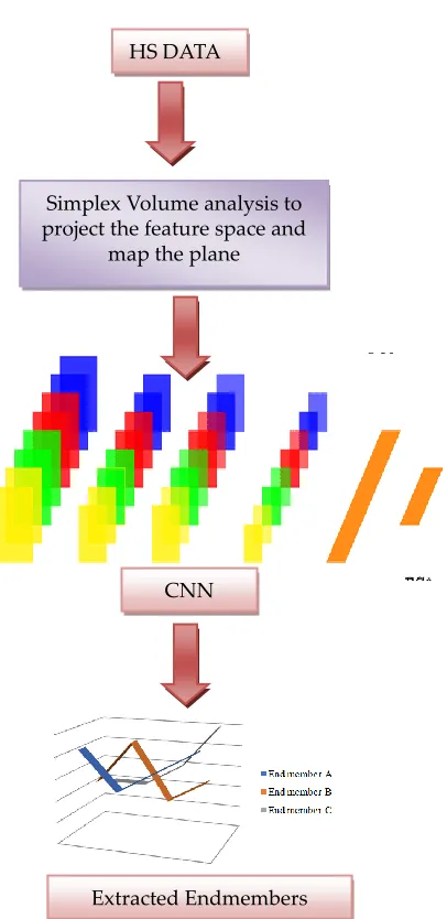
3. IS_CNN: ENDMEMBER EXTRACTION ALGORITHM
End member extraction is the key to unmix the spectral pure substances in a microscopic level of a pixel. The proposed method involves in identifying the endmembers where simple volume analysis method is often used in spectral non linear unmixing. The CNN method is known for the better image classification which is often experimented with combination of two or more convolutions and having advantages by addingmore layers for the in-depth study with the given real time data. The section 3.1 discusses about the procedure involved in building the IS_CNN algorithm.
3.1 Iterative Simplex Volume Analysis using Convolutional Neural Network (IS_CNN)
Assume S be a A x 1 observation spectrum of the column vector and EM= {e1, e2, ...., ek} be S x k matrix of the endmembers spectra. The equation (2) shows the formula for a simplex estimation k vertices e1, e2, ...., ek..
( 1, , . . . . , ) = (( 1) 1 | [1 1 … . . 1 ]|) … … … . ( )
Let k vertices e1, e2, ...., ek. of a simplex compose k-1 polyhedron edges as formulated as
P: {e2 – e1, ... ek – e1}and then equation (3) is equivalent to the volume of simplex
( 1, , … . , ) = ( 1) 1 √| ( | … … … . ( )
The feature space on simplex volume analysis is initialized by nonlinear mapping. In 𝒴 the original HS data are mapped which contains the huge dimensionality feature space F. Basically for dimensionality reduction minimum noise fraction (MNF) or Principal Component Analysis (PCA) techniques are used widely to reduce from A to the dimension k -1. For this study PCA technique is employed. Here ∅(𝑆) and ∅( ) are pixel vector and end member vector respectively in the F.
∅: 𝑆 ∈ 𝒴 → ∅(𝑆) ∈ 𝐹 … … … … … … . (4)
If T is a randomly generated target pixel then the simplex volume equation (5) in F is shown below
(∅( ), … . , ∅( )) = ( 1) 1 √| (( ∅ )
∅ | … … . ( )
The iteration i← 1:k end member vertices : matrix construction of the equation (5) will be updated to N ← N+1 (Where N: {1,2...}). This loop will be repeated till it satisfies the condition N= k constraint.
The CNN is involved to identify the target endmember pixels T from the constructed matrix. As depicted the network of the CNN contains seven layers Input, Convolutional layer 9x9 with nonlinear Sigmoid activation function, mean pool layer, stack layer, sigmoid with the dimension of 360, sigmoid with dimension of 60, softmax with dimension of 10 and cost function layer uses the cross entropy measure for extracting the endmembers. .
81
4 EXPERIMENTAL RESULTS AND DISCUSSION
The AVIRIS Indian Pine Hyperspectral dataset is used for this study to analyze the performance of the IS_CNN algorithm. The HS dataset contain 16 classes as per the ground truth information and with dimension of 145 x 145 x 220. Here 145 X 145 is the continuous spectral values for each band of 220. The proposed algorithm is compared with the FCLS nonlinear unmixing approach. Initially before estimating FCLS in a supervised manner the mixing matrix has to generate with the combination two end members estimated signatures. At last, the FCLS method is applied to the generated matrix to calculation the fraction of pure substances present in a pixel. The root mean squared error (RMSE) is obtained after extraction of the endmembers is considered as the performance measure. For FCLS, the RMSE is used to find the similarity from the estimated to true fraction of substances [20]. The Table 1 and Figure 3 shows the ground truth information for the AVIRIS Indian Pines HS data.
Figure 3: Ground truth with labels for AVIRIS Indian pine Hyperspectral Data
Table 1. Indian pines ground truth dataset with respective number of samples for each class
Table 2: RMSE is measured for two endmember extraction algorithms
Label Class No. of
Samples
1 Alfalfa 54
2 Corn-no till 1434
3 Corn-min till 834
4 Corn 234
5 Grass Pasture 497
6 Grass-Trees 747
7 Grass-Pasture-Mowed 26
8 Hay-Windrowed 489
9 Oats 20
10 Soybean-no till 968
11 Soybean-min till 2468
12 Soybean-clean 614
13 Wheat 212
14 Woods 1294
15
Buildings-Grass-Trees-Drives 380
16 Stone steel -Towers 95 Simplex Volume analysis to
project the feature space and map the plane
HS DATA
CNN
Extracted Endmembers
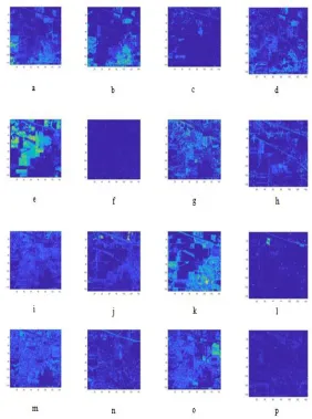
The results from the Table 2 shows that in FCLS, the extracted endmembers Alfalfa, Corn-no till, Corn-min till, Corn, Grass Pasture, Grass-Trees, Grass-Pasture-Mowed, and Hay-Windrowed RMSE measure is 0 and the overall average RMSE for FCLS is 0.18. The proposed IS_CNN method obtained the slightest error in all the extracted end members but still overall RMSE average is 0.08 which shows the significance performance in extracting the endmembers when compared to the FCLS. The Figure 4 shows the reconstructed image after the extraction of end members for the AVIRIS Indian pine HS data.
Figure 4: AVIRIS Indian pine image reconstruction after extracting the endmembers through IS_CNN: a) Alfalfa b)
Corn-no till c) Corn-min till d) Corn e) Grass Pasture f) Grass-Trees g) Grass-Pasture-Mowed h) Hay-Windrowed i)
Oats j) Soyabean-no till k) Soyabean-min till l) Soybean-clean m) Wheat n) Woods o) Buildings-Grass-Trees-Drives p)
Stone steel –Towers
5
C
ONCLUSION ANDF
UTUREW
ORKThe subpixel-wise classification especially in nonlinear mixing substances per pixel are often decrease the performance of the classification. Endmembers extraction and abundance mapping are the two stages of Hyperspectral nonlinear unmixing. Over the decades there are different nonlinear unmixing approaches are conducted based on the statistical algorithms and few on the classification techniques. In recent years, CNN, and Deep neural networks are experimented with nonlinear mixing Hyperspectral data to increase the performance of the accuracy. The FCLS and the novel proposed IS_CNN method are experimented with the AVIRIS Indian Pine dataset and proved that the average RMSE of the proposed method is much lesser than the FCLS method. This proposed algorithm involves with the
End Members FCLS IS_CNN
Alfalfa 0.00 0.01
Corn-no till 0.00 0.01
Corn-min till 0.00 0.03
Corn 0.00 0.04
Grass Pasture 0.00 0.05
Grass-Trees 0.00 0.05
Grass-Pasture-Mowed 0.00 0.05
Hay-Windrowed 0.00 0.07
Oats 0.14 0.08
Soybean-no till 0.17 0.09
Soybean-min till 0.27 0.13
Soybean-clean 0.28 0.14
Wheat 0.39 0.16
Woods 0.45 0.16
Buildings-Grass-Trees-Drives
0.53 0.17
Stone steel -Towers 0.64 0.17
83 traditional CNN technique to map the endmembers. In future
this research work will be extended to map the fraction of abundances by employing novel or hybridized deep neural networks.
Acknowledgements
This research study is supported under the University Research Fellowship (URF NO: C2/2016/2170) from theBharathiar University, Coimbatore, India.
References:
[1] Nirmal Keshava, ― A survey of spectral unmixing algorithms‖ , Lincoln Laboratory journal, Vol 14 (1), 2003.
[2] Miao Li, Shuying Zang, Bing Zhang, Shanshan Li & Changshan Wu (2014) A Review of Remote Sensing Image Classification Techniques: the Role of Spatio-contextual Information, European Journal of Remote Sensing, 47:1, 389-411, DOI: 10.5721/EuJRS20144723.
[3] Jie Yu, Dongmei Chen, Yi Lin & Su Ye (2017) Comparison of linear and nonlinear spectral unmixing approaches: a case study with multispectral TM imagery, International Journal of Remote Sensing, 38:3, 773-795, DOI: 10.1080/01431161.2016.1271475
[4] Liangrocapart, S., and Maria Petrou. "Mixed pixels classification." Image and Signal Processing for Remote Sensing IV. Vol. 3500. International Society for Optics and Photonics, 1998.
[5] Carmen Quintano , Alfonso Fernández-Manso , Yosio E. Shimabukuro & Gabriel Pereira (2012) Spectral unmixing, International Journal of Remote Sensing, 33:17, 5307-5340, DOI: 10.1080/01431161.2012.661095
[6] Nascimento, José MP, and José M. Bioucas-Dias. "Nonlinear mixture model for hyperspectral unmixing." Image and Signal Processing for Remote Sensing XV. Vol. 7477. International Society for Optics and Photonics, 2009.
[7] Heylen, Rob, Mario Parente, and Paul Gader. "A review of nonlinear hyperspectral unmixing methods." IEEE Journal of Selected Topics in Applied Earth Observations and Remote Sensing 7.6 (2014): 1844-1868.
[8] Cui, Jiantao, Xiaorun Li, and Liaoying Zhao. "Nonlinear spectral mixture analysis by determining per-pixel endmember sets." IEEE Geoscience and Remote Sensing Letters 11.8 (2014): 1404-1408.
[9] Zhao, Liaoying, et al. "Fast implementation of linear and nonlinear simplex growing algorithm for hyperspectral endmember extraction." Optik 126.23 (2015): 4072-4077.
[10] Halimi, Abderrahim, et al. "Nonlinear unmixing of hyperspectral images using a generalized bilinear model." IEEE Transactions on Geoscience and Remote Sensing 49.11 (2011): 4153-4162.
[11] Halimi, Abderrahim, et al. "A new Bayesian unmixing algorithm for hyperspectral images mitigating endmember variability." 2015 IEEE International Conference on Acoustics, Speech and Signal Processing (ICASSP). IEEE, 2015.
[12] Altmann, Yoann, Nicolas Dobigeon, and Jean-Yves Tourneret. "Unsupervised post-nonlinear unmixing of
hyperspectral images using a Hamiltonian Monte Carlo algorithm." IEEE Transactions on Image Processing 23.6 (2014): 2663-2675.
[13] Ammanouil, Rita, et al. "Nonlinear unmixing of hyperspectral data with vector-valued kernel functions." IEEE Transactions on Image Processing 26.1 (2017): 340-354.
[14] Ayerdi, Borja, and Manuel Graña. "Hyperspectral image nonlinear unmixing and reconstruction by ELM regression ensemble." Neurocomputing 174 (2016): 299-309.
[15] Ayoobi, Iman, and Majid H. Tangestani. "Evaluation of subpixel unmixing algorithms in mapping the porphyry copper alterations using EO-1 Hyperion data, a case study from SE Iran." Remote Sensing Applications: Society and Environment10 (2018): 120-127.
[16] Chakravorthy, Somdatta. "Analysis of end member detection and subpixel classification algorithms on hyperspectral imagery for tropical mangrove species discrimination in the Sunderbans Delta, India." Journal of Applied Remote Sensing7.1 (2013): 073523.
[17] Close, Ryan, et al. "Using physics-based macroscopic and microscopic mixture models for hyperspectral pixel unmixing." Algorithms and Technologies for Multispectral, Hyperspectral, and Ultraspectral Imagery XVIII. Vol. 8390. International Society for Optics and Photonics, 2012.
[18] Palsson, Burkni, et al. "Hyperspectral unmixing using a neural network autoencoder." IEEE Access 6 (2018): 25646-25656.
[19] Zhang, Xiangrong, et al. "Hyperspectral unmixing via deep convolutional neural networks." IEEE Geoscience and Remote Sensing Letters 99 (2018): 1-5.