R E G U L A R A R T I C L E
Open Access
Crime event prediction with dynamic
features
Shakila Khan Rumi
1*, Ke Deng
1and Flora Dilys Salim
1*Correspondence:
1School of Science, Computer
Science and Information Technology, RMIT University, Melbourne, Australia
Abstract
Nowadays, Location-Based Social Networks (LBSN) collect a vast range of information which can help us to understand the regional dynamics (i.e. human mobility) across an entire city. LBSN provides unprecedented opportunities to tackle various social problems. In this work, we explore dynamic features derived from Foursquare check-in data in short-term crime event prediction with fine spatio-temporal granularity. While crime event prediction has been investigated widely due to its social importance, its success rate is far from satisfactory. The existing studies rely on relatively static features such as regional characteristics, demographic information and the topics obtained from tweets but very few studies focus on exploring human mobility through social media. In this study, we identify a number of dynamic features based on the research findings in Criminology, and report their correlations with different types of crime events. In particular, we observe that some types of crime events are more highly correlated to the dynamic features, e.g.,Theft,Drug Offence,
Fraud,Unlawful EntryandAssaultthan others e.g.Traffic Related Offence. A key challenge of the research is that the dynamic information is very sparse compared to the relatively static information. To address this issue, we develop a matrix factorization based approach to estimate the missing dynamic features across the city. Interestingly, the estimated dynamic features still maintain the correlation with crime occurrence across different types. We evaluate the proposed methods in different time intervals. The results verify that the crime prediction performance can be significantly improved with the inclusion of dynamic features across different types of crime events.
Keywords: Crime event prediction; Dynamic features; Matrix factorization
1 Introduction
Crime event prediction is important to crime prevention in the society by helping the law enforcement agencies to design optimal patrol strategies. Reduction of crime events will benefit society in numerous ways. It will increase the public safety and decrease the economic loss. However, crime event prediction is a challenging task [1]. The spatial and temporal distributions of crime events differ from one type to the other. As shown in Fig.1, we can observe the difference in the spatial distribution of three different types of crime event, i.e.,Theft,Drug Offence, andAssaultrespectively in Brisbane. Many factors are rel-evant to the possibility that a particular type of crime event is going to occur in a region
Figure 1Spatial distribution of different types of crime event in Brisbane
in the near future. These include demographics, the distribution of different types of ser-vices, crime history, human mobility and so on.
Traditionally, crime event prediction uses the historical patterns of crime events, the information collected from geographic information systems (GIS) and demographic vari-ables, e.g. sex, income, age, and race and so on. But these variables are almost constant or only change slowly over time. Therefore, they do not capture the short-term variations of the factors which are relevant to the occurrence of crime events [2]. With the widespread use of social media such as Twitter and Foursquare in the last decade, large volumes of information have been generated which provide unprecedented opportunities to capture the city dynamics, i.e. human mobility across a city [3]. A few researchers take advan-tage of Twitter data to assist crime event prediction [4–6]. They capture the sentiments of neighborhoods by topic analysis of Twitter data. While the sentiments change over time, it typically takes a relatively long time to identify the change. According to some urban research [7], the diversity of visitors to a location and associated influences over time are directly relevant to an area’s safety and one can obtain such high dynamic information on human mobility from LBSN data. But they are ignored largely in crime event prediction. This work attempts to fill the gap.
For a given city withRregions (known asmeshblocksorcensus regions), we aim to iden-tify the regions where a certain type of crime event will happen in the next time interval. Several types of crime event are studied includingTheft,Unlawful Entry,Drug Offence,
Traffic Related Offence,Fraud, andAssault. The criminal offence which includes the il-legal taking of other persons belonging without consent to permanently or temporarily deprive the owner is defined asTheft. When a person enters a building (e.g. office, bank, shop etc.) with an intention to commit crime can be classified asUnlawful Entry.Drug Offenceincludes any form of sale, dealing, importing or exporting, manufacture or culti-vation of illegal drugs or other substances. The offences which are related to most forms of road traffic, including pertaining to the licensing, registration, road worthiness or use of vehicles, bicycle offences, and pedestrian offences can be classified asTraffic Related Of-fence. According to the Queensland Police,aFraudis a type of behavior towards a person or organization which is deceptive, dishonest, corrupt or unethical. All types of physical and mental harm towards a person are defined asAssault. This includes all types of phys-ical contact with a person without their consent.
cate-gories: historical, demographic, geographic and dynamic. We derive the historical features from the crime event records. They describe the density and trend of crime event in a re-gion and the surrounding rere-gions. The demographic features reflect the socio-economic conditions of residents in a region. The geographic features retain the information about the properties of venues in a region. While the crime event prediction has been studied by exploring historical, demographic, geographic features, the unique aspects of this work lies in the proposal of a series of dynamic features in crime event prediction. We extract the dynamic features from check-ins of Foursquare users. For a particular Foursquare user, the visiting history is associated with her/his habits and routines [8,9]. According to routine activity theory, the opportunities for crime events are optimized in places where victims and offenders come together in greater concentrations [10,11]. For example, a location with visitors from diverse backgrounds in a time interval is highly correlated with some types of crime event such asTheft; monitoring the fluctuation of visitor diversity at loca-tions provides useful information to the crime event prediction. The contribuloca-tions of this paper are summarized as follows:
• This work systematically explores highly dynamic human mobility from Location-Based Social Network to lift the crime event prediction performance. • This work identifies a number of dynamic features derived from Foursquare check-ins
based on the research findings in Criminology. On real data sets in Brisbane and New York City, we have conducted extensive tests with the widely used prediction models (including SVM, Random Forest, Neural Network, and Logistic Regression) and an ensemble model, and the widely used features (historical features, geographic features, demographic features) in existing crime event prediction studies. The prediction performance before and after adding the proposed dynamic features have been performed and compared. The test results demonstrate the improvement of
prediction performance after adding dynamic features is considerable and statistically significant.
• The dynamic features are highly sparse compared to the relatively static features. To handle this issue, we have developed a matrix factorization based approach to estimate the missing dynamic features across the city. Interestingly, the estimated dynamic features well retain the correlation with crime event occurrences of different types.
The rest of the paper is organized as follows. In Sect.2, we briefly introduce the related work in crime event prediction. Section3describes the data sets used in this study. Sec-tion4discusses the details of the prediction features and shows the correlations between dynamic features and different types of crime event. In Sect.5, the sparsity of dynamic fea-tures is addressed. The evaluation results on real data sets are reported in Sect.6. Finally, this work is concluded in Sect.7.
2 Related work
event occurrences. While the urban activities have argued that population diversity and visitors’ ratio contribute to an area’s safety [7,15], they change frequently due to human mobility. In our study, we have exploited the human mobility data from foursquare to rep-resent the human dynamics of a region for a short time period. Later, it has verified the impact of dynamic features on top of related constant features in short-term crime event prediction of various types. We have categorized the existing works into four following types.
2.1 Crime event prediction using historical information
Traditional methods for crime event prediction assume that crime events are most likely to happen in the vicinity of past crime events. For a given region, the historical data of a certain type of crime events is analyzed to predict the possibility of the crime event to happen in the near future (e.g. [1]). Various models have been developed over the past decade including regression model, machine learning techniques like Neural Networks, Support Vector Machine (SVM), One Nearest Neighbor (1NN), Decision Tree, Random Forest, and Ensemble Learning.
In [1], they focus onBurglaryprediction. The city is divided using a grid. For each grid cell, the number of Burglary in the past is counted by month. They run several classifiers including 1NN, J48, SVM, Neural Network and Naive Bayes to predict the possibility of
Burglaryin the next month for each grid cell based on the crime historical data in this cell and neighboring cells. It shows J48, SVM, Neural Network always outperform the others and Neural Network often performs better than J48 and SVM. But this model solely depends on the past history of crime events in the vicinity.
In [16] and its extended version [13], the authors propose a Cluster-Confidence-Rate-Boosting algorithm (CCRBoost) which concurrently considers the spatial and temporal factors as well as the relevant types of crime event. For example, a type of crime event, e.g.,
Robbery, is used as an indicator of the relevant crime event to be predicted, e.g.,Burglary. Different indicators of the same location in the same period of time are used to form a vector. Each vector has one class label which informs whether this location is a hot spot for the crime event to be predicted.
In [17], the authors use the theory of self-exciting point process (SEPP) method in crime prediction particularly in residential burglary prediction. SEPP is a popular approach for modeling space-time clustering of seismic activity. They demonstrate that a better pre-diction performance can be achieved using this model. Commercial software for crime prediction like PredPolbuses SEPP as an underlying algorithm. This tool predicts crime based on the location and time of past crime event data.
2.2 Crime event prediction using geographic and demographic information
the census information extracted from demographic data, and the temporal information (i.e. the number of months from the last occurrence of crime event).
Some crime prediction tool e.g, Hunchlab considers other information with historic in-formation. It is designed by GIS firm Azavea [18]. It takes account wider range of variables with near-repeat victimization. The variables include seasonality, social and environmen-tal risk factors.
2.3 Crime event prediction using social media
The above studies explore the geographic and demographic information observed over a long time period i.e. months. Some researchers further embedded the features extracted from social media data like Twitter in their prediction model. In [4], the probability of a certain type of crime event at a given location in a city is predicted by considering infor-mation in the surrounding regions from two aspects: the density of crime events of the same type and the topics of tweets in the surrounding regions. The density of crimes is evaluated using Kernel Density Estimation(KDE). The topics of the tweets in surrounding regions are modeled using Latent Dirichlet Allocation (LDA). Using the density as one feature and each topic as a separate feature, a logit model is trained.
In [5], the authors use topics from the tweets posted by local News Agencies for each day as a predictor of the occurrence of crime events in the following day using a General Linear Regression Model (GLM). In order to source the topics from tweets, Semantic Role Labelling (SRL) and LDA are applied. SRL is a method to extract events from tweets and these events form a document for each day. Since the number of events in a document can be very large, LDA method is applied to identify the topics for each document and calculate the probability of the document belonging to each topic. These topics are used as predictor in crime event occurrence in the following day. In [6], the authors extend their work [14] with the topics identified from tweets in [5]. But the information extracted from tweets in this work has a drawback. The tweets of News Agencies only contain information of breaking news. Many types of crime event such asTheftare ignored and many details are missing due to the limitation of the number of words in tweets.
2.4 Crime event prediction using human mobility
One study further consider human behaviors extracted from the mobile network activities and demography, for example, the number of people connecting the mobile networks in different regions over time [19]. In [20], the crime event interference problem takes advan-tage of Point Of Interest (POI) information to estimate the population distribution across a city and information of taxiflows to help understanding the spatial correlation between nearby places. In [21], the authors extend the work [20] by representing the temporal dy-namics and multihop transition using a flow graph; they combined the spatial graph and flow graph through a graph embedding method.
next time interval based on previous weight matrices. Finally, the number of crime is pre-dicted based on this weight matrices.
Recently, the crime event occurrences in New York City are studied using the features extracted from Foursquare data [23,24]. For a given region, the authors extract a number of features and verify the spatial correlation between the extracted features and the num-ber of crime events in a region in [23]. In [24], the authors measure the ambient population of a census region and analysis crime incidents from demographic point of view. Instead of crime event prediction, these two works focus on measuring the relationship between crime event occurrences and local features. In contrast, our study aims to verify the spatial and temporal correlation between the proposed dynamic features and the occurrence of a crime event in a region in the next time slot.
3 Data sets
Two data sets have been collected. One is from Brisbane, the capital city of Queensland, Australia and the other is from New York City, USA.
3.1 Brisbane
The crime event records of Queensland, Australia, are collected from the API available in Queensland government data websitecfrom 01/2013 to 09/2013. In the collected data, we focus on the section in Brisbane only. It provides the information on occurrence location and time of different types of crime events. There is a total 17 types of crime events in this data set. In this study, we select the 6 types of crime events introduced in Sect.1. The frequency distribution of these crime events isTheft(30.34%),Unlawful Entry(13.38%),
Drug Offence(8.85%),Traffic Related Offence(8.67% ),Fraud(4.13%) andAssault(3.71%). The geographic unit of this data set is census regions. There are total 13,161 census regions in Brisbane. The mean size of these regions is 0.082 km2which is very fine-grained spatial division. The demographic data of Brisbane is collected from Australian Bureau of Statistics.d
The Foursquare venue data and check-in data in Brisbane for the same time period as crime event records are obtained from the authors [25,26]. In these papers, they demon-strated that they filtered out noise and invalid check-ins from the foursquare datasets as much as possible. They filtered out noisy data using three different steps. First, they filtered the fake check-ins by analyzing the sudden movement of users. Second, they removed the check-ins with no venue information. Finally, they filtered out the check-ins of inactive users. Hence, the probability of propagation of noise across areas is minimal. The venue is also known asPoint Of Interest(POI). Foursquare venue data are static data which refer to the information relating to venues including the location in longitude and latitude for-mat and the category of service. We have a total of 4421 venues in Brisbane. Foursquare divides the venues into nine major categories. These areArtsandEntertainment, Col-lege and University,Food,NightLife Spot,Outdoor and Recreation,Professional and Other Places,Residential,Shop and Service, andTravel and Transport. The Foursquare check-in data are dynamic data which are the user check-ins at various venues. The data set consists of 20,454 check-ins performed by 611 users.
3.2 New York City
In New York City, the frequency distribution of these crime events isTheft(27.06%), Un-lawful Entry(3.95%),Drug Offence(6.82%),Traffic Related Offence(1%),Fraud(2.18%) andAssault(15.17%).
We partition the New York City by census regions as well. It consists of total 2166 re-gions. The mean size of these regions is 0.36 km2. The demographic data of New York City is collected from United States Census Bureau.fWe consider the population size for every census region of 2011 census.
The Foursquare venue data and check-in data in New York City for the same time pe-riod as crime event records of New York City are obtained from the authors of [27]. The authors have filtered out the noise using same steps described in Sect. 3.1. There are a to-tal of 43,964 venues in New York City. As in Brisbane, they are organized into nine major categories. There are about 0.23 million (i.e., 227,428) check-ins performed by 1083 users.
4 Prediction features
We now introduce the features used in crime events prediction which are categorized into four categories: historical features, geographic features, demographic features, and dynamic features.
4.1 Historical features
According to near-repeat theory in criminology research, the crime events are more likely to happen in the vicinity of past crime events [28]. To retain the historical knowledge about crime event occurrence, we calculate features based on the crime event density for each regionr. Suppose the current date isdand the next time interval istnext.
4.1.1 α-Days crime event density
Crime events are generally concentrated in few locations. According to near hotspots, the crime event that has happened recently can be described by the previous near crime events [29]. Theα-days crime event density characterizes the recent crime event distribution. It is based upon the number of crime events at regionrduring time intervaltin the past α days. Since the area size and the population size of different regions are not uniform, it is improper to use the number of crime events only [30]. So, we normalize crime event density by area size and population size respectively:
DAi(r,tnext) =
d
j=d–αCrj(r) A(r) ,
DPi(r,tnext) =
d
j=d–αCrj(r) P(r) ,
(1)
where Crj(r) is the number of crime events occurred at dayjin regionrduring time
inter-valt;A(r) andP(r) are the area size and population size of regionrrespectively. In this work, we consider both 7-days and 30-days crime event density, i.e.,α= 7 andα= 30.
4.1.2 Crime event trend
historical data, and then the sliding window moves ahead day-by-day until the starting time isd–α. For the sliding window at each starting time, the crime event density is de-fined as the ratio between the number of crime events happened in the sliding window and the number of days of the sliding window. The trend is modeled using polynomial regression of order 2. Crime is a rare event. It does not happen regularly in a certain place. It causes fluctuations in the dataset. Hence, polynomial regression is required to model the trend of crime event density in a region. The trend can be modeled using polynomial regression of order 2 or higher. For simplicity the trend is modeled using polynomial re-gression of order 2. The crime events density of the sliding window covering the nextw
days after the current datedis computed, and the average is used as the crime event trend.
4.1.3 Neighborhood crime event density
According to [31], the crime rate in one region can be influenced by the crime rate of its neighborhood regions. The neighborhood crime event density reflects the situation of surrounding regions. We check the spatial correlation of crime event occurrence by cal-culating theMoran Iindex. We test it for crime typeTheft,AssaultandDrug Offence. In theMorantest, we use the binary weight matrix which assigns weight 1 for all neighbour regions and zero otherwise. Observing the test results, we found positiveMoran I statis-tics for each type of crime event. It indicates that there is a spatial autocorrelation be-tween neighbourhoods in terms of crime event densities. Specifically, the nearby regions have more impact on each other than other regions. TheMoran Istatistic forAssaultis
p= 0.572 while this value forTheftisp= 0.153. The lowpvalue indicates the findings are statistically significant. This indicates that the regions of occurringAssaultare more clustered thanTheft. This situation can also be visually observed in Fig.1.
For each adjacent region, theα-days crime event density is computed and the average of all adjacent regions is used as the neighborhoodα-days crime event density. For each adjacent region, the crime event density trend is calculated and the average of all adjacent regions is used as the neighborhood crime event density trend.
For each adjacent region, theα-days crime event density is computed and the average of all adjacent regions is used as the neighborhoodα-days crime event density. For each adjacent region, the crime event density trend is calculated and the average of all adjacent regions is used as the neighborhood crime event density trend.
4.1.4 Seasonal crime event density
Previously, seasonal patterns have been observed in some crime types e.g., Assault [32]. Inspiring from this we calculate seasonal crime event density for each type of crime event. The season of the current date is considered. For regionrin time intervaltnext, the crime event density of the same season is computed and divided by the number of days of the season, i.e., the average number of crime events per day in this season is used as the sea-sonal crime event density.
4.2 Geographic features
The geographic features describe the regional information of Foursquare venues in each region including venue category density, venue category distribution, and regional diver-sity.
Table 1 Spearman’s rank correlation coefficients between POI categories and crime event types
POI Category Type of crime event
Drug Offence Assault Unlawful Entry Theft Fraud
Arts and Entertainment 0.39 0.39 0.25 0.43 0.42
College and University 0.13 0.24 0.29 0.41 0.09
Food 0.35 0.38 0.27 0.4 0.37
NightLife Spot 0.51 0.48 0.15 0.47 0.36
Outdoor and Recreation 0.2 0.23 0.09 0.14 0.04
Professional and Other Places 0.28 0.32 0.15 0.37 0.34
Residential 0.03 0.18 0.06 0.03 0.02
Shop and Services 0.4 0.47 0.36 0.49 0.51
Travel and Transport 0.3 0.37 0.15 0.39 0.3
Table 2 Spearman’s rank correlation coefficients between theft and POIs at different time intervals
Time Interval
POI Category Arts and Entertainment
College and University
Food Nightlife Spot
Outdoor and Recreation
Professional and Other Places
Residential Shop and Service
Travel and Transport
[0–3) 0.38 0.33 0.35 0.51 0.12 0.35 0.03 0.43 0.41
[3–6) 0.19 0.18 0.27 0.58 0.06 0.3 0.02 0.23 0.28
[6–9) 0.39 0.47 0.31 0.37 0.12 0.36 0.03 0.34 0.37
[9–12) 0.44 0.32 0.31 0.39 0.15 0.32 –0.004 0.48 0.43
[12–15) 0.48 0.5 0.38 0.38 0.12 0.36 0.01 0.5 0.3
[15–18) 0.48 0.3 0.37 0.28 0.18 0.25 0.02 0.49 0.37
[18–21) 0.41 0.38 0.38 0.35 0.07 0.29 0.03 0.45 0.3
[21–24) 0.35 0.15 0.29 0.47 0.16 0.3 0.11 0.25 0.39
in the regions where at least one venue of that venue category situates. The results are shown in Table1for Brisbane. ForDrug OffenceandAssault, the most correlated POI category isNightLife Spot; forTheftandFraud, the most correlated POI category isShops and Service. The results are consistent with the obvious facts [33,34]. TheResidentialarea is least correlated with any type of crime event.
We also examine the Spearman’s rank correlation coefficient in different time intervals. Table2illustrates that forTheftagainst different venue categories. The most correlated venue category isShops and Servicewithin the interval [9–21), and isNightlife Spot includ-ingNightclubandBar within the interval [21–6). The other venue categories are much weakly correlated withTheftat all time intervals.
4.2.1 Venue category distribution
As shown in Table1, different venue categories have different impacts to different types of crime event at different time intervals. For example, crime events will be likely to hap-pen at night near the night life spots. Previous studies also showed that Drug Offence, Assault normally happens near Bar [34] or other nightlife spots where Theft type of crime events mostly happens in shopping areas [33]. We calculate the number of venues for each category. The nine venue categories considered are shown in Table1. Venue category dis-tribution is defined as follows:
Pi(r) = Ni(r)
N(r), (2)
whereNi(r) is the number of venues of categoryiin regionrandN(r) is total number of
4.2.2 Venue category density
For regioni, venue category density is calculated as
Di(r) = Ni(r)
A(r), (3)
whereNi(r) is the number of venues of categoryiin regionrand the area size of the region
isAi. The intuition behind is that density of venues (without considering categories of
venues) is correlated to the number of crime events in the same region [20].
4.2.3 Regional diversity
To quantify the venue heterogeneity of regionr, we apply Shanon’s Entropy measure [35]. The entropy of regionris calculated as follows:
H(r) = –
i∈P
Ni(r) N(r)×log
Ni(r) N(r)
, (4)
whereNi(r) is the number of venues of categoryiin regionrandN(r) is the total number of
venues in regionr. Generally, the area with high entropy is expected to be diverse in terms of venues, that is, the number of venues of different categories are similar; the area with low entropy is expected to be less diverse, i.e., the number of venues of some categories dominates that of other categories. The intuition behind is that a diverse location may attract the crime events offenders. The intuition behind is that a diverse location attract different groups of people. It also describes variety of usage of a region (shop, college). Such diversity index is good predictor in crime event prediction model [19]. The similar entropy has been applied for identifying the optimal locations for new retail stores by calculating the entropy of the locations inside a certain radius [36].
4.3 Demographic features
Previous studies have shown that the crime event occurrences in a place are correlated with the socioeconomic and demographic features of this location and its neighborhood area [19,20]. Figure2illustrates the demographic information across the Brisbane city
including the number of residents, median age, median income and gender ratio in each region. We can observe that the number of residents in most regions is between 0 and 500. A few regions have more than 500 residents. It also illustrates median age and me-dian income distribution for each region. If comparing the crime event distribution shown in Fig.1, we can visually observe that crime event happens where median age of the popu-lation is respectively low in general. It indicates that the young popupopu-lation is more related to the crime event than the aged population. Also, we can observe that crime events are more likely to occur in low income regions. Similarly, we can see that crime events are more likely to occur in the regions where the number of females are less than the num-ber of males. The other demographic features that we also consider are the fraction of stable population, rented household, diversity of ethnic background, and diversity of in-come.
4.4 Dynamic features
Urban activists have argued that the population diversity and visitor ratio contributes to an area’s safety [7,15]. Due to human mobility, the population diversity and visitor ratio always change over time. To capture the dynamics, we explore Foursquare check-ins to obtain six featuresVisitor Ratio,Region Popularity,Visitor Entropy,Visitor Homogeneity,
Observation Frequency, andVisitor Count. In particular, the last four features have been used to measure the social diversity in other studies [37–41].
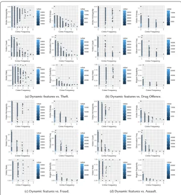
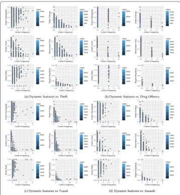
We show the correlation between the dynamic features and different types of crime events including Theft, Drug Offence, Assault, Fraud for time interval [15:00–18:00) (Fig.3) and for time interval [21:00–24:00) (Fig.4) in New York City. Note that any point (x,y) in the two figures, only ifx= 0 andy= 0, corresponds to a region where dynamic fea-tures exist and this type of crime event occurs in the specified time interval. Even though the number of such points is limited, interesting information can be observed.
The hexbin plots show no linear correlation between the features and the crime event frequency. In most cases, no crime event occurs no matter the values of dynamic fea-tures is high or low. It is consistent with the fact that the crime event of all types are typi-cally rare. However, we can still observe the crime events are more likely to happen when the dynamic features fall in a range of values. For example, whenVisitor Entropyis 0.5,
Theftis much more likely to happen compared to whenVisitor Entropyis near 1 or less than 0.1.
4.4.1 Visitor entropy
The diversity of population in a location describes the area’s safety. Visitor Entropy reflects the diversity of visitors in a location with respect to his visits. Such entropy has been used in [37] to measure the social diversity. Shanon’s entropy measure can be used to quantify to which extent the visitors to a venue are frequent visitors. For regionrat time interval
t, the entropy is defined as follows:
H(r,t) = –
u∈U(r)
Pr,t(u)log2Pr,t(u), (5)
wherePr,t(u) is the probability that useruvisits regionrand its neighborhood at time
Figure 3Correlation between dynamic features and crime event occurrences in the interval [15–18) in New York City
time intervalt. The high visitor entropy of a region at a certain time interval means that many visitors are not frequent visitors; the low entropy means many visitors are frequent visitors.
As shown in Figs.3and4, whenVisitor Entropyis near 1, the crime event of different types are less likely to happen; whenVisitor Entropyis less than 0.5, the situation becomes complex.
4.4.2 Visitor homogeneity
Figure 4Correlation between dynamic features and crime event occurrences in the interval [21–24) in New York City
dimension corresponds to a venue category. We use pairwise cosine similarity between the visitors in the high dimension space. The visitor homogeneity in the regionrand its neighborhood at time intervaltis measured as follows:
HMi(r,t) =
u,v∈U(r,t)sim(u,v)r,t
U(r,t) . (6)
whereU(r,t) is the set of all visitors who visit regionrand its neighborhood at time interval
tandsim(u,v)r,tis the cosine similarity between two visitors inU(r,t).
As illustrated in Figs.3and4, whenVisitor Homogeneityis over 0.25 the crime events are less likely to happen forDrug Offence,Assault,Fraud. ForTheft, the situation is complex. But it still indicates the lowVisitor Homogeneityimplies the higher possibility ofTheft.
4.4.3 Region popularity
opportunity [10,11]. To assess the popularity of regionrat time intervalt, we count the number of check-ins observed in the region at that time interval, and then divide it by the total number of check-ins observed in all regions at the same time interval, that is:
RP(r,t) = |C(r,t)|
r∈R|C(r,t)|
. (7)
whereC(r,t) is the total check-ins at time intervaltandRis the set of all regions in the city.
Figure3and4indicateRegion Popularityis a good indicator of crime event. When the value ofRegion Popularityis over 0.3, the crime event is very unlikely to happen for all crime types; when the value ofRegion Popularityis less than 0.3, the possibility of crime event occurrence increases markedly.
4.4.4 Visitor ratio
The visitor ratio of a regionrat time intervaltis defined as follows:
VRr,t=| V(r,t)|
|C(r,t)|, (8)
whereV(r,t) denotes the number of check-ins by new users in regionrand its neighbor-hood atttime intervals, andC(r,t) is the total check-ins at time intervalt. To do that, we first find the four most visited venues of each Foursquare user since on average a people only visits 2–4 places regularly [42]. Then for each check-ins we check whether it is a new venue for this visitor. If it is, the relevantV(r,t) is increased by 1.
Even though there is not clear value boundary, the higherVisitor Ratiovalue shows the trend of the higher probability of crime event occurrence as demonstrated in Figs.3and 4.
4.4.5 Visitor count
The number of unique users in regionrat time intervalt,|U(r,t)|, is defined asVisitor Count. It gives the absolute number of visitors.Visitor Counthas been used as a feature to measure the diversity of location [38]. We use this feature into our problem to reflect location diversity dynamically in crime event prediction. According to the correlation be-tweenVisitor Countand crime events as presented Figs.3and4, whenVisitor Countis less than 2, a crime event is more likely to happen for different crime event types.
4.4.6 Observation frequency
We also consider|C(r,t)|, i.e., the number of check-ins in regionrand its neighborhood at time intervalt, as a dynamic feature.Observation FrequencyandRegion Popularityare related more and less. WhileObservation Frequencyis the absolute number,Region Pop-ularityis a relative number. WhenObservation Frequencyis less than 3, the crime event of different types are much more likely to happen compared to that when Observation Frequencyis over 3.
5 Crime event prediction
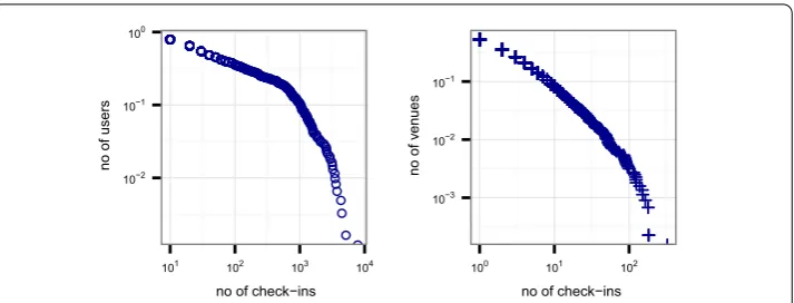
Figure 5Complementary cumulative distribution function (CCDF) of check-ins in Brisbane
About 10% of venues have 10 check-ins and 1% of venues have 100 check-ins. Even though the correlation between the dynamic features and the crime events exists as shown in Fig.3 and Fig.4, the dynamic features are missing in many time intervals of many regions. As a result, when training a prediction model for a particular crime type at a particular time interval, it is hard to find many useful regions at this time interval where dynamic features exist and this type of crime occurs. Note that any point (x,y) in Fig.3and Fig.4correspond a useful region only ifx= 0 andy= 0. This situation seriously limits the practical value of dynamic features in crime event prediction. It is essential to address this issue first.
5.1 Dynamic feature estimation
Suppose two regionsr1andr2have the similar dynamic features at many different time intervals. If the dynamic feature inr1is missing at a time interval but is known inr2at the same interval, it is reasonable that we estimate the value inr1 from the value inr2. Suppose the dynamic features of the same region at two time intervalst1andt2, for ex-ample [14:00, 14:20] and [16:20, 16:40], are similar over many days. If the dynamic feature of this region in time intervalt1is missing in one day but is known in time intervalt2in the same day, it is reasonable that we estimate the missing value int1from the value in
t2. Motivated by the recommender system [43], we use collaborative filtering technique to estimate the missing dynamic features. Specifically, the latent factor model based on matrix factorization is applied.
Matrix factorization models map both time intervals and regions to a joint latent factor space of dimensionalityf, such that interactions between time intervals and regions are modeled as inner products inf. Accordingly, each time intervaliis associated with a vector
qi∈Rf, and each regionuis associated with a vectorpu∈Rf. In the resulting dot product qT
ipu, the approximation of regionu’s dynamic features at different time intervali, denoted
asrui, leads to the estimate
ˆ
rui=qTi pu. (9)
To learn the factor vectors (puandqi), the system minimizes the regularized squared error
on the set of known dynamic features:
min
q,p
(u,i)∈K
rui–qTipu 2
+λqi2+pu2
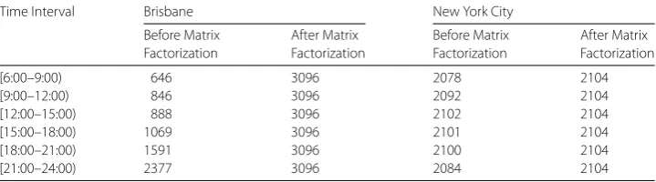
Table 3 Number of regions with dynamic features
Time Interval Brisbane New York City
Before Matrix Factorization
After Matrix Factorization
Before Matrix Factorization
After Matrix Factorization
[6:00–9:00) 646 3096 2078 2104
[9:00–12:00) 846 3096 2092 2104
[12:00–15:00) 888 3096 2102 2104
[15:00–18:00) 1069 3096 2101 2104
[18:00–21:00) 1591 3096 2100 2104
[21:00–24:00) 2377 3096 2084 2104
whereKis the set of the (u,i) pairs for whichruiis known (the training set). The system
learns the model by fitting the known dynamic features. However, the goal is to general-ize those known dynamic features in a way that estimates the missing dynamic features. Thus, the system should avoid over-fitting the known dynamic features by regularizing the learned parameters, whose magnitudes are penalized. The constantλcontrols the extent of regularization and is usually determined by cross-validation. We setλ= 0.001 and op-timize the cost function until converge. Table3shows the number of regions in different time intervals before and after matrix factorization.
We observe that the correlations after matrix factorization are highly similar to that before matrix factorization as shown in Figs.3and4. It means that the estimated dynamic features can be effectively used in crime event prediction. If a region does not have any check-in at all time intervals, the dynamic features cannot be estimated and thus the crime event prediction in this region cannot be explored by dynamic features. Such regions are ignored in this work. Again, to prevent the extreme sparse data, we ignore the regions where less than 10 check-ins have been observed in the whole time period. We also remove the time intervals when the number of check-ins is generally low and needs to be filled in large number. Particularly, it includes the time period between 1 am–6 am.
5.2 Ensemble method
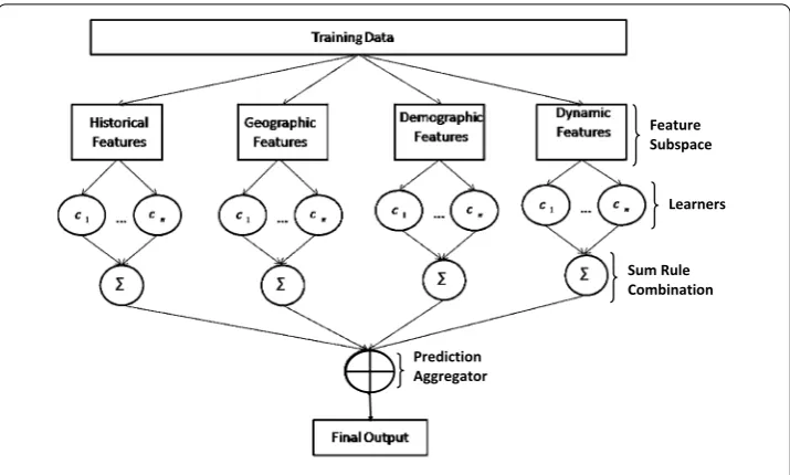
We select four prediction models which are Random Forest (RF), Neural Network (NN), kernel Support Vector Machine (SVM), Logistic Regression Model (LR). Besides these, we also use an ensemble based learning framework for crime event prediction. The structure of the ensemble method is demonstrated in Fig.6. It takes the following four steps.
• The first step divides the training space based upon the types of the features. For our problem, we divide the training space into four subsets, i.e., historical, geographic, demographic and dynamic, to provide different views in the prediction model. • The second step builds classifiers using different learning algorithms for each
non-overlapping training subset (each subset corresponding to one set of features). In our problem, the feature space is high dimensional and from heterogeneous sources. When we divide the feature space based on feature types, it may create linear and non-linear combination of features. Hence, in our proposed ensemble model, we choose different combination of learning algorithms including linear model,
kernel-based model, tree-based model and ensemble model. We selected the popular classifier algorithms of these models as component classifiers. In particular, we choose Support Vector Machine (SVM) as a kernel-based model, Classification and
Figure 6Ensemble model for crime event prediction
model and Linear Discriminant Analysis (LDA) as a linear model. These classifiers are denoted asc1, . . . ,cnin Fig.6and explained below in more detail.
•Support Vector Machine (SVM) This is a binary classifier which non-linearly maps the input vectors to a high-dimensional space [44]. A linear decision surface is constructed in this space where the margin between the training patterns and the decisions boundary tends to be maximized. Several kernel function including Polynomial, Radial Basis Function (RBF) and Perceptrons are used to serve this purpose [45].
•Classification and Regression Tree (CART) This is a tree based learning algorithm which constructs classification or regression tree based on the dependent vari-ables [46]. If the dependent variables are categorical, it constructs the classifica-tion tree; if the dependent variables are numerical, it constructs the regression tree. CART creates rules for splitting the data at a node based on one variable. After splitting the data, recursion is applied in the child node until stopping rules are found. Finally, the leaf nodes generate the final prediction.
•Linear Discriminant Analysis (LDA) This is another binary classification algo-rithm which separates the classes based on the linear combination of the predic-tors [47]. LDA model assumes that each of the predictors has the same variance. It calculates the mean and variance of the predictors for each class based on this assumption.
•Random Forest (RF) This is an ensemble learning method which constructs multi-ple decision trees (ntree) in a random subspace of the feature space [48]. For each
subspace, the unpruned tree generates their classifications and in the final step, all the decisions generated byntreeare combined for final prediction [49].
this work is
Os=
j∈C
Ojs, (11)
whereCis set of classifiers andOjsis the outcome of classifierjon training subsets.
• The fourth step aggregates the outcomes of each feature subsets for the final outcome. We train an SVM learning algorithm to aggregate the predictions made by each training subset.
6 Experiments
In this section, the experiment results are reported and discussed. The data used in the experiments is introduced in Sect.3. The aim of the experiments is to examine the effec-tiveness of the dynamic features to crime event prediction at different settings.
6.1 Data preparation
First, we partition a day into 3 hours interval. Given a region, we predict whether it will be a hot spot in the next time interval for a particular type of crime (in other words, predict whether at least one crime event of a particular type will happen in this region in the next interval). Most of the existing works focused on comparatively long term crime prediction e.g. 1 day, 1 year. With the aim for short-term crime event prediction a day is divided into total eight intervals and each interval spans 3 hours. Crime prediction in finer temporal grain will help the police to design their patrol strategies dynamically and it will increase the probability to reduce crime rate more effectively. The shorter span of time interval, e.g., 1 hour, is better for short-term crime prediction. However, crime is a rare event and inter-sharing time of check-ins is high. Hence, we aggregate 3-hours interval data in our study.
As discussed in Sect.5, it is hard to find many regions within a specified time interval where dynamic features exist and a particular type of crime event occurs. This makes it difficult to train a useful prediction model. So, the matrix factorization based method is applied to estimate the missing dynamic features as discussed in Sect.5.1. In this exper-iment, the prediction models with dynamic features are trained after the estimation of missing dynamic features.
We partition the data in about 70% as the training set and the rest 30% as the test set for both cities, Brisbane and New York City. Particularly, in Brisbane, the data lies be-tween 01/02/2013–30/06/2013 is considered as the training set and bebe-tween 01/07/2013– 16/09/2013 as the test set. In New York City, the training set involves the data between 03/03/2012–31/10/2012 and the data between 01/11/20112–15/02/2013 are test set.
Most of the existing crime event prediction models used AUC, F1-score, Accuracy as their evaluation metrics [4,13,19]. Hence, In this paper we have chosen the Area Under Curve (AUC) under Receiver Operating Characteristic (ROC) curve, Accuracy, F1-score as the evaluation metrices.
6.2 Effectiveness of dynamic features
Five prediction models have been applied. They are the Random Forest (RF), Neural Net-work (NN), kernel Support Vector Machine (SVM), Logistic Regression Model (LR), and the introduced ensemble method (Ensemble). In particular, the Radial Basis Function (RBF) kernel is used in SVM. RBF is a real-valued function which calculates the Euclidean distance of the input variables from its origin [51]. We measure the performance of each model trained on combination of the historical, geographic and demographic features and then combining them with the dynamic features, for different types of crime event includ-ingTheft,Drug Offence,Assault,Fraud,Unlawful EntryandTraffic Related Offenceduring different time intervals.
6.2.1 Brisbane
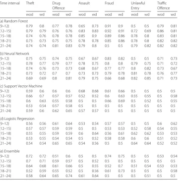
The test results of AUC values with RF, NN, SVM, LR and Ensemble models are shown
in Table 4. We observe the improvement of the AUC values after adding the dynamic
features within different time intervals for different types of crime event. While the pre-diction performance varies based on the type of crime event and time interval for most of the prediction models, the RF shows the consistent improvement of AUC values after adding the dynamic features. In specific, with RF within different time intervals, the AUC values increase up to 4% after considering the dynamic features forTheft, 4% forDrug Offence, 16% forAssault, 2% forFraud, and 6% forUnlawful Entry. No improvement has been observed forTraffic Related Offence. The test results verify that the dynamic features are significant to predict different types of crime event except forTraffic Related Offence. Interestingly, RF also possesses the best AUC values for all types of crime event within dif-ferent time intervals. RF algorithm is consistent and adapts to sparsity. The convergence rate of the algorithm depends on only the strong features and hence, it is independent on the noise variables in the model [52]. For further evaluation, we report Accuracy% and F-1 score% with RF model in Table5. We observe that the models with dynamic features yield better Accuracy% and F-1 score% than the models without dynamic features within different time intervals for different types of crime events.
6.2.2 New York City
Table 4 AUC comparison with and without dynamic features for Brisbane (“wod” and “wd” represent without and with dynamic features respectively)
Time interval Theft Drug Offence
Assault Fraud Unlawful
Entry
Traffic Offence
wod wd wod wd wod wd wod wd wod wd wod wd
(a) Random Forest
[9–12) 0.79 0.8 0.77 0.78 0.65 0.73 0.91 0.9 0.5 0.5 0.79 0.81
[12–15) 0.79 0.79 0.76 0.76 0.83 0.83 0.92 0.91 0.72 0.69 0.86 0.81
[15–18) 0.74 0.76 0.78 0.78 0.85 0.9 0.89 0.86 0.78 0.8 0.83 0.81
[18–21) 0.73 0.73 0.75 0.75 0.78 0.78 0.85 0.86 0.78 0.8 0.82 0.82
[21–24) 0.74 0.74 0.81 0.83 0.79 0.8 0.5 0.5 0.79 0.82 0.82 0.82
(b) Neural Network
[9–12) 0.75 0.75 0.74 0.75 0.67 0.67 0.83 0.82 0.5 0.5 0.71 0.73
[12–15) 0.78 0.77 0.79 0.77 0.78 0.75 0.8 0.8 0.79 0.75 0.71 0.72
[15–18) 0.74 0.76 0.73 0.73 0.68 0.67 0.77 0.77 0.8 0.82 0.73 0.67
[18–21) 0.73 0.72 0.7 0.7 0.73 0.73 0.79 0.78 0.81 0.78 0.76 0.77
[21–24) 0.69 0.69 0.8 0.81 0.79 0.75 0.66 0.68 0.82 0.85 0.71 0.73
(c) Support Vector Machine
[9–12) 0.59 0.6 0.6 0.6 0.68 0.68 0.61 0.66 0.5 0.5 0.5 0.5
[12–15) 0.66 0.7 0.57 0.57 0.52 0.52 0.6 0.63 0.55 0.55 0.5 0.58
[15–18) 0.6 0.63 0.55 0.58 0.5 0.5 0.66 0.69 0.5 0.52 0.5 0.55
[18–21) 0.53 0.54 0.57 0.58 0.5 0.5 0.5 0.5 0.5 0.5 0.5 0.5
[21–24) 0.59 0.6 0.62 0.65 0.57 0.57 0.5 0.5 0.5 0.5 0.5 0.5
(d) Logistic Regression
[9–12) 0.56 0.56 0.61 0.64 0.53 0.54 0.57 0.57 0.5 0.5 0.6 0.62
[12–15) 0.57 0.57 0.59 0.59 0.5 0.5 0.53 0.53 0.52 0.58 0.54 0.55
[15–18) 0.55 0.55 0.59 0.59 0.6 0.64 0.56 0.61 0.62 0.62 0.53 0.53
[18–21) 0.53 0.55 0.54 0.54 0.5 0.52 0.58 0.58 0.6 0.6 0.51 0.52
[21–24) 0.54 0.54 0.65 0.65 0.54 0.56 0.5 0.5 0.64 0.64 0.52 0.52
(e) Ensemble
[9–12) 0.72 0.72 0.51 0.6 0.5 0.5 0.74 0.75 0.5 0.5 0.53 0.54
[12–15) 0.7 0.71 0.59 0.57 0.5 0.52 0.5 0.5 0.5 0.5 0.5 0.5
[15–18) 0.64 0.68 0.61 0.66 0.5 0.55 0.52 0.7 0.51 0.54 0.53 0.53
[18–21) 0.52 0.59 0.55 0.52 0.5 0.56 0.61 0.73 0.5 0.5 0.5 0.58
[21–24) 0.58 0.64 0.65 0.74 0.61 0.64 0.5 0.5 0.5 0.51 0.5 0.5
Table 5 Metrics comparison with and without dynamic features for Brisbane (“wod” and “wd” represent without and with dynamic features respectively)
Time interval Theft Drug Offence
Assault Fraud Unlawful
Entry
Traffic Offence
wod wd wod wd wod wd wod wd wod wd wod wd
(a) Accuracy%
[9–12) 96.14 95.41 90.6 98.57 96.55 98.11 96.65 94.88 86.78 95.8 90.28 97.37 [12–15) 96.57 96.86 90.93 98.68 96.61 98.03 96.54 96.37 86.78 95.8 90.14 96.67 [15–18) 94.4 94.4 91.2 98.75 96.59 98.43 97.98 94.34 89.86 96.69 90.1 96.4 [18–21) 93.63 96.28 90.73 97.79 96.45 98.88 97.56 95.04 87.54 97.11 89.55 97.75 [21–24) 92.88 97.96 90.65 98.57 96.45 98.3 97.54 95.6 86.45 95.84 90.01 97.19 (b) F-1 Score%
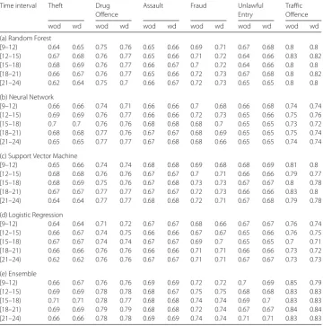
Table 6 AUC comparison with and without dynamic features for New York City. “wod” and “wd” represent without and with dynamic features, respectively
Time interval Theft Drug Offence
Assault Fraud Unlawful
Entry
Traffic Offence
wod wd wod wd wod wd wod wd wod wd wod wd
(a) Random Forest
[9–12) 0.64 0.65 0.75 0.76 0.65 0.66 0.69 0.71 0.67 0.68 0.8 0.8
[12–15) 0.67 0.68 0.76 0.77 0.65 0.66 0.71 0.72 0.64 0.66 0.83 0.82
[15–18) 0.68 0.69 0.76 0.77 0.66 0.67 0.7 0.72 0.64 0.66 0.8 0.8
[18–21) 0.66 0.67 0.76 0.77 0.65 0.66 0.72 0.73 0.67 0.68 0.8 0.82
[21–24) 0.62 0.64 0.75 0.7 0.66 0.67 0.72 0.73 0.65 0.65 0.8 0.8
(b) Neural Network
[9–12) 0.66 0.66 0.74 0.71 0.66 0.66 0.7 0.68 0.66 0.68 0.74 0.74
[12–15) 0.69 0.69 0.76 0.77 0.66 0.66 0.72 0.73 0.65 0.66 0.75 0.76
[15–18) 0.7 0.7 0.76 0.76 0.68 0.68 0.68 0.7 0.65 0.65 0.73 0.72
[18–21) 0.68 0.68 0.77 0.76 0.67 0.67 0.68 0.69 0.65 0.65 0.75 0.74 [21–24) 0.65 0.65 0.77 0.77 0.67 0.68 0.68 0.66 0.65 0.65 0.74 0.74 (c) Support Vector Machine
[9–12) 0.65 0.66 0.74 0.74 0.68 0.68 0.69 0.68 0.68 0.69 0.81 0.8
[12–15) 0.68 0.68 0.76 0.76 0.67 0.67 0.7 0.71 0.66 0.66 0.79 0.77
[15–18) 0.68 0.69 0.75 0.76 0.67 0.68 0.73 0.73 0.67 0.67 0.8 0.78
[18–21) 0.67 0.67 0.77 0.77 0.67 0.67 0.72 0.73 0.66 0.66 0.83 0.8 [21–24) 0.64 0.64 0.77 0.77 0.68 0.68 0.72 0.71 0.67 0.68 0.79 0.78 (d) Logistic Regression
[9–12) 0.64 0.64 0.71 0.72 0.67 0.67 0.68 0.66 0.67 0.67 0.76 0.74
[12–15) 0.66 0.67 0.74 0.75 0.66 0.66 0.67 0.67 0.65 0.66 0.76 0.75
[15–18) 0.67 0.67 0.74 0.74 0.67 0.67 0.69 0.7 0.65 0.65 0.7 0.71
[18–21) 0.66 0.66 0.76 0.76 0.66 0.66 0.71 0.71 0.66 0.66 0.73 0.72 [21–24) 0.62 0.62 0.76 0.76 0.67 0.67 0.71 0.71 0.67 0.67 0.73 0.73 (e) Ensemble
[9–12) 0.66 0.67 0.76 0.76 0.69 0.69 0.72 0.72 0.7 0.69 0.85 0.79
[12–15) 0.69 0.69 0.78 0.78 0.68 0.67 0.75 0.75 0.68 0.68 0.83 0.83
[15–18) 0.71 0.71 0.78 0.77 0.68 0.68 0.74 0.74 0.69 0.7 0.83 0.83
[18–21) 0.69 0.69 0.79 0.79 0.68 0.68 0.72 0.74 0.67 0.67 0.84 0.84 [21–24) 0.66 0.66 0.78 0.78 0.69 0.69 0.74 0.74 0.71 0.71 0.83 0.83
reported in Table7. Same as Brisbane, the models with dynamic features yield better Ac-curacy% and F-1 score% than the models without dynamic features within different time intervals forTheft,Drug Offence,AssaultandFraud. The performances slightly decrease within some time intervals forUnlawful EntryandTraffic Related Offence.
6.3 Significance test
Table 7 Metrices comparison with and without dynamic features for New York City (“wod” and “wd” represent without and with dynamic features respectively)
Time interval Theft Drug Offence
Assault Fraud Unlawful
Entry
Traffic Offence
wod wd wod wd wod wd wod wd wod wd wod wd
(a) Accuracy%
[9–12) 69.55 72.55 77.14 78.05 68.0 69.86 64.86 64.07 63.84 64.61 72.73 72.04 [12–15) 73.39 76.22 75.42 77.1 67.07 68.68 67.41 67.86 62.16 60.21 72.32 71.4 [15–18) 74.63 76.56 77.96 78.85 68.54 70.31 67.05 67.84 61.72 61.59 72.96 71.69 [18–21) 72.46 75.07 74.58 75.59 67.49 69.6 67.05 66.02 61.56 59.74 71.6 70.55 [21–24) 67.32 69.01 74.22 76.0 68.46 69.72 69.05 67.49 63.28 75.12 71.3 69.7 (b) F-1 Score%
[9–12) 81.83 83.89 87.08 87.65 80.87 82.14 78.64 78.05 77.86 78.44 84.2 83.74 [12–15) 84.36 86.25 85.92 87.01 80.15 81.3 80.48 80.8 76.6 75.09 83.93 83.3 [15–18) 85.18 86.46 87.55 88.1 81.17 82.42 80.22 80.79 76.26 76.15 84.35 83.49 [18–21) 83.73 85.5 85.33 86.0 80.42 81.92 80.26 79.5 76.15 74.74 83.44 82.71 [21–24) 80.26 81.46 85.1 86.27 81.12 82.01 81.68 80.58 77.47 78.84 83.23 82.13
Table 8 Estimatedp-value for different crime types at different time interval
Time Interval Theft Drug
Offence
Assault Fraud Unlawful
Entry
Traffic Related Offence (a) Brisbane
[9–12) 0.04 0.95 0.172 0.02 0.81 0.81
[12–15) 0.002 0.589 0.828 0.019 0.97 0.97
[15–18) 0.01 0.01 0.987 0.02 0.189 0.19
[18–21) 0.189 0.631 0.877 0.83 0.4 0.04
[21–24) 0.01 0.048 0.1 0.828 0.4 0.42
(b) New York City
[9–12) 1.5e–8 0.005 1.68e–7 0.0007 0.31 0.31
[12–15) 2.84e–8 3.09e–7 1.44e–6 0.0001 0.05 0.03
[15–18) 2.2e–7 3.45e–5 1.09e–5 0.002 0.31 0.02
[18–21) 2.2e–7 5.12e–6 6.94e–9 0.03 0.006 0.001
[21–24) 4.25e–7 9.15e–6 1.73e–7 0.03 0.02 0.01
of the time intervals in both cities. It proves that the dynamic features are significant in
Theftprediction. Conversely, largerp-value forTraffic Related Offenceat some time inter-vals justifies that dynamic features are less significant to predict this type of crime event. For the other types of crime event, the significance of the dynamic features depends on time interval and city. We can observe that the improvement after adding the dynamic features are statistically significant for more types of crime event within different time in-tervals in New York City than Brisbane. It proves that the availability of fineness human mobility data increases the significance of dynamic features in predicting different types of crime event.
6.4 Individual dynamic feature
For the different types of dynamic feature, the effectiveness in crime event prediction is not the same. We evaluate the importance of each individual dynamic feature to predict a crime event. In particular, we report the test result forTheftprediction. However, the same analysis can be applied to the other types of crime event.
experi-Table 9 The AUC with and without individual dynamic feature forTheftprediction
Dynamic Features Brisbane New York City
[15–18) [21–24) [15–18) [21–24)
wod wd wod wd wod wd wod wd
Visitor Homogeneity 0.807 0.808 0.770 0.794 0.676 0.681 0.626 0.628
Visitor Entropy 0.807 0.818 0.770 0.785 0.676 0.680 0.626 0.629
Region Popularity 0.807 0.810 0.770 0.769 0.676 0.679 0.626 0.632
Visitor Ratio 0.807 0.823 0.770 0.788 0.676 0.676 0.626 0.628
Visitor Count 0.807 0.812 0.770 0.777 0.676 0.679 0.626 0.625
Observation Frequency 0.807 0.809 0.770 0.771 0.676 0.675 0.626 0.626
wod: without dynamic features; wd: with dynamic features.
ments. The experimental results are shown in Table9. The higher values of the AUC un-der ROC curve of these results show the extent to which the dynamic feature improves the prediction performance. While we observe a significant improvement in most of the cases in these results, the effectiveness of each dynamic feature varies with respect to time interval and city. In particular,Visitor Homogeneityis the most important dynamic feature for Brisbane (4.8% improvement in AUC) and New York City (1% improvement in AUC) within the interval [21–24) and [15–18), respectively. On the other hand,Region Popular-ityandVisitor Ratioare the most important features for New York City (1.2% improvement in AUC) within the interval [21–24) and Brisbane (3.2% improvement in AUC) within the interval [15–18), respectively. We also observe thatRegion PopularityandVisitor Count
show a slightly decreased AUC values for Brisbane and New York City, respectively, within the interval [21–24), which indicates them as a noise inTheftprediction. The fact that different dynamic features may prove more or less significant across cities, types of crime event, and time intervals signifies that the problem of crime event prediction is not trivial.
6.5 Static vs. dynamic features
The effectiveness of all features (including static and dynamic) is investigated with LR for
Theftprediction. To make it comparable, all features are normalized in between 0 and 1 [20]. The coefficient of each feature in the LR model indicates the importance of the cor-responding feature. The most important 12 features (6 positives and 6 negatives) in two time intervals are shown in Table10for Brisbane and New York City. The positive coef-ficient means that the feature is positively correlated with the occurrence of crime events and the negative coefficient denotes the opposite. We observe that historical features have the strongest correlation with the occurrence of crime event. In Brisbane, we observe that the most positively correlated feature is30-days crime densitywhile the most negatively correlated feature is7-days crime densityfor both intervals. In New York City, they are sea-sonal densityand30-days crime densityrespectively. It reveals an interesting pattern that
Thefthappens in the same region but less frequently. That is, it does not happen weekly but happen monthly in Brisbane and it follows a seasonal pattern in New York City.
For the dynamic features within the interval [15–18),Visitor Counthas positive corre-lation withTheftwhereasRegion PopularityandVisitor Homogeneityare negatively cor-related withTheftin Brisbane. It is interesting that the opposite happens within the inter-val [21–24). In New York City,Observation Frequencyis positively correlated withTheft
Table 10 The most correlated features withTheft
[15–18) pm [21–24) pm
Positive coefficient Negative coefficient Positive coefficient Negative coefficient (a) Brisbane
30-days Crime Density (Population based) (1.1e+02)
7-days Crime Density (Population based) (–1.1e+02)
30-days Crime Density (Population based) (52.67)
7-days Crime Density (population based) (–52.5) Seasonal Crime Density
(0.71)
Visitor Homogeneity (–0.43)
Seasonal Crime Density (1.3)
Visitor Count (–0.61)
Visitor Count (0.56) 30-days crime Density (Area based) (–0.39)
Visitor Homogeneity (0.67)
Gender Ratio (–0.32) Location Diversity (0.32) Median Income (–0.16) 30-days Crime Density
(Area based) (0.66)
Median Income (–0.13) Gender Ratio (0.27) Region Popularity
(–0.12)
Median Age (0.4) POI Category Distribution (Outdoor and Recreation) (–0.08)
POI Category Distribution (Shop and Services) (0.266)
7-days Crime Density (Area based) (–0.12)
Region Poularity (0.356) POI Category Distribution (College and University) (–0.06)
(b) New York City Seasonal Crime Density (0.99)
30-days Crime Density (Area based) (–0.35)
Seasonal Crime Density (2.12)
30-days Crime Density (Area based) (–2.14) 7-days Crime Density
(Population based) (0.36)
POI Category Distribution (Nightlife) (–0.17)
30-days Crime Density (Population based) (1.17)
7-days Crime Density (population based) (–0.71) Gender Ratio (0.27) 30-days Crime Density
(Population based) (–0.13)
Gender Ratio (0.22) Visitor Entropy (–0.095)
Regional Diversity (0.26) POI Category Distribution (Travel and Transport) (–0.09)
Venue Category Density (0.17)
Median Age (–0.06)
Rented House (0.18) POI Category Distribution (Outdoor and Recreation) (–0.06)
Observation Frequency (0.16)
Ethnic Diversity (–0.05)
Observation Frequency (0.16)
Visitor Ratio (–0.05) Economic Diversity (0.157) POI Category Distribution (Travel and Transport) (–0.04)
withTheftwithin the interval [15–18), which isVisitor Entropywithin the interval [21– 24).
7 Conclusion
This work assists in solving the crime event prediction problem with its focus on explor-ing relevant dynamic features. Specifically, we propose to use the features extracted from human mobility to represent the dynamics of a region. Compared with previous studies on crime event prediction where relatively static features were the focus, this work was motivated by the research findings in Criminology which hold that many human-related factors such as social diversity and population distribution are relevant to an area’s safety. By capturing human mobility data through social media, it allows us to improve crime event prediction in finer spatiotemporal granularity.
beyond the scope of the aimed research problems and will shed light on the field of spa-tiotemporal data analysis.
In future, we plan to extend our work in multiple ways. One of them is instead of verify-ing the model usverify-ing data of same city only; we can use data from one city as trainverify-ing data and other one as test data. This could place the model verification in better way. However, the data distributions of different cities are vastly different. Hence, the problem needs to be formulated from transfer learning and domain adaptation point of view.
Acknowledgements
We thank all the CRUISE members for helpful discussion.
Funding
Not applicable.
Abbreviations
AUC, Area Under Curve; CARET, Classification and Regression Tree; CCDF, Complementary Cumulative Distribution Function; CCRBoost, Cluster-Confidence-Rate-Boosting; GAM, General Additive Model; GIS, Geographic Information System; GLM, General Linear Regression Model; KDE, Kernel Density Estimation; LBSN, Location Based Social Network; LDA, Latent Dirichlet Allocation; LDA, Linear Discriminant Analysis; LR, Linear Regression; NN, Neural Network; POI, Point of Interest; RBF, Radial Basis Function; RF, Random Forest; ROC, Receiver Operating Characteristic; SRL, Semantic Role Labeling; SVM, Support Vector Machine; 1NN, One Nearest Neighbor.
Availability of data and materials
Data and materials are available upon request.
Competing interests
The authors declare that they have no competing interests.
Authors’ contributions
SKR, KD and FS equally scoped the research. SKR formulated the initial idea, conducted the computational experiments and drafted the manuscript. KD and FS revised the problem formulation, guided the experiments and drafted the manuscript. All authors read, edited and approved the final manuscript.
Endnotes
a https://www.police.qld.gov.au/
b http://www.predpol.com/how-predictive-policing-works/
c https://data.qld.gov.au
d http://www.abs.gov.au/
e https://data.cityofnewyork.us/Public-Safety/
f https://www.census.gov/about/regions/new-york.html
Publisher’s Note
Springer Nature remains neutral with regard to jurisdictional claims in published maps and institutional affiliations.
Received: 27 February 2018 Accepted: 7 October 2018
References
1. Yu C-H, Ward MW, Morabito M, Ding W (2011) Crime forecasting using data mining techniques. In: 2011 IEEE 11th international conference on data mining workshops, pp 779–786
2. Cohn EG (1990) Weather and crime. Br J Criminol 30(1):51–64
3. Zheng Y, Capra L, Wolfson O, Yang H (2014) Urban computing: concepts, methodologies, and applications. ACM Trans Intell Syst Technol 5(3):38
4. Gerber MS (2014) Predicting crime using Twitter and kernel density estimation. Decis Support Syst 61(1):115–125 5. Wang X, Gerber MS, Brown DE (2012) Automatic crime prediction using events extracted from Twitter posts. In:
International conference on social computing, behavioral-cultural modeling, and prediction. Springer, Berlin, pp 231–238
6. Wang X, Brown DE, Gerber MS (2012) Spatio-temporal modeling of criminal incidents using geographic, demographic, and Twitter-derived information. In: Intelligence and security informatics (ISI), 2012 IEEE international conference on, pp 36–41. IEEE
7. Jacobs J (1961) The death and life of American cities