Volume-7 Issue-2
International Journal of Intellectual Advancements
and Research in Engineering Computations
Information retreival complex query mapping on multi agent cloud
Mrs.B.Deepa
1, S.Rashma
2, R.Rubana
2, N.Sandiya
21
Assistant Professor, Department of Computer Science and Engineering, Nandha Engineering
College
2
UG-Students, Department of Computer Science and Engineering, Nandha Engineering College
ABSTRACT
Mining large data requires intensive computing resources and data mining expertise, which might be inaccessible to most of the users. With the regularly obtainable cloud computing resources, data mining tasks cannot be stimulated to the cloud or outsourced to the third party to save cost. In this new pattern, data and model confidentiality becomes the major un ease to the data owner. Data owners have to understand the possible trade-offs among client-side costs, model quality, and confidentiality to justify outsourcing solutions. In this paper, we propose the RASP Boost framework to address these problems in confidential cloud-based learning. The RASP-Boost approach works with our previous developed Random Space Data Perturbation (RASP) method to protect data confidentiality and uses the boosting framework to conquer the complexity of learning high-class classifiers as of RASP disconcerted data. So, we have to build up some cloud-client combined boosting algorithms. These algorithms need low client-side calculation and communication expenses. The client does not call for to stay online in the progression of learning models. So, we have methodically studied the confidentiality of data, model, and learning process under a realistic security model. Experiments on public datasets illustrate that the RASP-Boost approach can give high-quality classifiers, while preserving high data and model confidentiality and require low client-side expenses.
Keywords:
Cloud Computing, Scheduling, Optimization, Workflows, Resource capacity, Resource provisioning, Deadline, Virtualization, Virtual Machine, Auto-scaling, Consolidation, Mutation.INTRODUCTION
OLAP
A winning company nowadays has several decisions to formulate. The enhanced those decisions are entire, the further unbeaten, and gainful, the company is. To many leading decision makers, the ability to analyse faster and better than the competition resources better decisions, developed profitability, and more success. Optimization of the relational database (RDB) has enable many companies to ably accumulate the data about dealings, giving decision maker extra knowledge to utilize. However, there is a higher boundary to the quantity of data that one can have in an RDB and at a standstill achieve a resourceful
study on. The On-Line Analytical Processing (OLAP) allow user to carry out rapid and effectual study on great amounts of data.
The data are stored in a multi-dimensional method that more openly models genuine business data. And OLAP too allows users to contact summary data earlier and easier. They can then drill down into the summary records to get more detailed data, if need be. For a more detailed explanation of the OLAP rules.
field are analysed, and a significant outline of the product and/or product line is specified. Furthermore, issues connected to data-mining and data-warehouses are addressed.
OLAP system workings
An OLAP structure is integrated of numerous works. A top-level sight of the system includes a data source, an OLAP server, and a client. The data source is actually the source of data going to be analysed. Data from the basis are transferred or mocked keen on the OLAP server, anywhere it is prearranged and prepared to offer short query times. The client is the user interface to the OLAP server. In this segment, the role of each part and the implication in the complete system is described.
The source in an OLAP system is the server that stores the data to be analysed. Depending on the use of the OLAP product, the source could be a data warehouse, a legacy database housing company data, a collection of spread sheets that holds business data, or a grouping of any of the above. The capability of an OLAP product to work with data from a number of sources is very important. Requiring that all source data is stored in a particular format or in a confident database is problematic for database administrators. It too reduces the authority and suppleness of the OLAP product. Administrators and users find that OLAP products that allow data mining from not only a wide selection of sources, but multiple sources, are more flexible and useful than those that have additional needs.
Server
It is the back-end of an OLAP system of the OLAP server. This is what does all of the work (depending on the model of the system), and where data that is dynamically accessed is stored. Dissimilar philosophies preside over the architecture of the server. In particular, a major feature of an OLAP product is whether the server uses a multi-dimensional database (MDDB) to stock up the data, or a relational database (RDB). This section labels pros and cons to all approach.
MOLAP
The MOLAP stand meant for Multidimensional On-Line Analytical Processing. This way that the server uses an MDDB to stock up data. Because most OLAP products are based on and the term OLAP regularly refers to MOLAP as well. The purpose for using an MDDB is evenly open. It can ably store data that are by temperament multidimensional, provided so as to a resource of fast querying of the database. Data are transmitted from a data source (as described above) into the multidimensional database, and then the database is aggregated. This recalculation is actually what allows the OLAP queries to be quicker, since the computation of summary data is formerly done. The query time converts a function solely of the time required to access one piece of data, as opposed to the time to access many pieces of data and performing the computation. This approach also chains the philosophy of undertaking the work once, and by means of the results completed. Multidimensional databases are a quite new technology. All The uses of MDDBs bear the alike drawbacks that mainly new technologies do. Namely, they are not as robust as RDBs, and are not as enhanced to the same extent. An added disadvantage is that most multidimensional databases are incapable to be used while aggregating data, so it frequently takes point in time for new information to adapt on hand for study.
ROLAP
MDDBs do. They are intended for huge amounts of data. A main argument next to RDBs is that querying a huge database with SQL to obtain summary data typically resulted in multifaceted queries. skilled SQL computer operator could easily connection up valued system resources attempting to implement a query that is very simple in a MDDB.
Application OLAP
This is by future the largest area, and is generally what is thought of or referred to by the term OLAP. Application OLAP frequently consists of a multidimensional database that is to be accessed by an exacting application, or maybe multiple applications. There is Vendors in this area which is mainly offer clients for the database. The client can just be a viewer, or it can be a healthy application that provides the user a lot.
Iceberg query
Data mining is the development of evaluating data from different perspective and shortening it keen on useful information - the information that can be used to boost income, cuts costs, or together. Data mining software is the one of a number of analytical tools used for analyzing data. Data mining software allows the users to analyze data from many diverse magnitude or approaches, group it, and summarize the relationships acknowledged. Precisely, data mining is the process of ruling relationships or else patterns between dozens of fields in huge relational databases. Data mining software analyze associations and patterns in stored transaction data based on open-over user queries. More than a few types of analytical software are accessible statistical, machine learning, and neural networks.
Data mining brings a allotment of reimbursement to businesses, society, governments, sales, marketing, insurance, health care, transportation and medicine and so on.
Market Segmentation
Recognize the general features of clients who buy the same products from your company.
Fraud Detection
Discover which transactions are most likely to be falsified.
Direct Marketing
Make out which scenario must be integrated in a transmitting listing to acquire the uppermost response frequency.
Banking/Finance
Used to identify client consistency by analyzing the data of customer purchasing activities. Interactive marketing compute what each individual accessing a Web site is most likely interested in seeing.
Data mining relationship
Data mining covers of some of four types of relationships are sought Classes Stored data is used to find data in prearranged groups. For example, a restaurant sequence could source client purchase data to define when clients visit and what they typically order. This information might be used to enlarge traffic by having daily specials. Clusters Data items are grouped according to logical relationships or consumer preferences. For example, data can be mined to spot market segments or consumer affinities.
Associations
The Data can be mined to classify associations. The beer-diaper example is an example of associative mining Sequential patterns Data is mined to anticipate behavior patterns and leanings. For example, outside tools seller might guess the probability of a backpack being purchased based on consumer's purchase of sleeping bags and hiking shoes.
attribute grouping occurs in the database, or the smallest amount, highest, sum or average value of some attribute. Queries are performed on the cube to recover decision hold up information. Lately, introduced the CUBE operator for appropriately supporting multiple aggregates in OLAP database. CUBE operator is the n-dimensional generation of group-by operator. It computes group-by consistent to all possible combinations of a list of features.
In this work, we presented a tactic to efficiently answer joint queries on both structured and text types of data. The records which are in data warehouses are usually extracted from other database systems and consequently contain only what is known as structured data. A huge quantity of text document is insufficient for processing ingeniously joint queries over structured and text data. a proposal for providing quick approximate answers to the iceberg query is devised with the purpose of helping the user refine the threshold before issuing the “final” iceberg query with the suitable threshold. That is, it tries to eradicate the need of a domain expert or histogram statistics to make a decision whether the query will actually return the preferred “tip” of the iceberg. This tactic for upcoming with the exact threshold is complementary to the efficient processing of iceberg queries. This paper gives passing introduction about data mining used of data mining and its events. This paper presents a complete survey on the existing most important information about the evaluation of iceberg queries, the need for ice berg queries and algorithm employed for evaluation of iceberg queries. The objectives of iceberg queries are calculated in this paper. This gives us the future direction to work on efficient evaluation of iceberg queries. The main objective of Iceberg queries is to retrieve data quickly. The query optimization is the cleansing process in database administration and it help carry down speed of carrying out. Data mining techniques are often measured by their speed. The reason behind this that the faster the tool can run and the larger the data set which it can be applied. The Iceberg queries are usually very elite to calculate as they require more than a few scans of relationships.
Sequence databases
This provides a multiplicity of way to query the data and bioinformatics analysis tools to help facilitate genetic study. The basic association of these databases has bent the way computer-based molecular biology research is conducted. This chapter will put up an understanding of series databases by reviewing data storage space, ordinary tools and online resources linking to these resources. If the laboratory is the groundwork of untried biology, nucleotide sequence databases are the foundation of genomic bioinformatics. These databases provide raw genetic data, nucleotide sequence, and a variety of resources to extract information from it. Simple questions relating to subjects such as presence or absence of homologous sequences, amount of genetic data available for an organism, and literature related to genes can be answered through the nucleotide sequence databases. First and foremost, these database provide a complete resource for publicly available nucleotide sequence data.
genetic data encountered in many online databases and bioinformatics research applications.
The most informative area of the GBFF is the Features Table. As described in the introductory section, the features in the table are used by all of members of the INSDC. One or more qualifiers may accompany each of the feature elements, which allows for a further description of it. The feature is aligned to the left side of the document with the corresponding sequence located directly across; the qualifiers are listed directly below separated by a forward slash To assist with annotations, data contributors are asked to provide as much of the feature information as possible before submitting the entry keen on the database. Web Feat at EBI and the Sequin Help documentation at Gen Bank, both listed in Table 1, assist with the annotation process by outlining the features and qualifiers needed for a successful database entry. Three important Features of the Features Table are Source, Gene, and CDS (Coding Sequence). Source is the only required feature of the table and one of the few features with a mandatory qualifiers. Source depicts the natural source of the series start with the necessary life form qualifier. Some of the optional qualifiers include cell_ line, plasmid, gender, strain, tissue type etc. Gene is described as a range in the nucleotide sequence that has been identified as a gene, for which there is a corresponding name. The gene qualifiers include allele, map, product and partial. CDS describes an area of a sequence that has been translated from a nucleotide chain to a sequence of amino acids.
Probabilistic algorithm
The applicability of these probabilistic methods to strong control is currently restricted by the information that the sample generation is possible only in very special cases which include systems exaggerated by real parametric indecision bounded in rectangles or spheres. Sampling in more general indecision sets is normally performed during over bounding, at the expense of an exponential rejection rate. In this paper, randomized algorithms for solidity and performance of linear time invariant uncertain systems described by a general - pattern are considered. In particular, efficient polynomial-time algorithms for indecision
other contributions attacked the same problem following a parallel line of research, with the goal of computing upper and lower bounds (instead of the “true” value) of the toughness edge for very general feedback configurations. In extra terms, the local point of these papers is to develop either necessary or sufficient conditions for robust stability and performance. The nice feature of these bounds is that their evaluation generally requires the solution of convex programs which can be easily performed. In this setting, is indeed bounded in a given set, but it is also a random matrix with a given probability distribution. In this way, both probabilistic and deterministic information is captured. In this paper, the class of so-called radically symmetric distributions in excess of the insecurity set is studied.
RELATED WORKS
Previous studies on privacy-preserving data mining (PPDM) are often based in the context of sharing data and mined models without leaking individual data records. Thus, the confidentiality of data and model is not the major concern, but the private information hidden in the shared data is. Three groups of techniques have been developed in PPDM. (1) Additive perturbation techniques that hide the real values by adding noises. Because the resultant models are not protected, they are not appropriate for outsourced mining. (2) Cryptographic protocols that enable multi-party collaborative mining without leaking either party‟s private information. These protocols typically do not move the original data to another party, but exchange intermediate results, which are proved not breaching data privacy. However, the learned models are shared by the participants. (3) Data anonymization that disguises personal identities or virtual identifiers in the shared data. It only protects personal identities, while the sensitive attributes and the resultant models are not protected. Some of the PPDM work also targets on outsourced mining, such as geometric data perturbation and random projection perturbation, which can be applied to cloud-based or data-mining-service based mining. They typically transform both the data and the learned models, trying to protect the confidentiality of both. The
dataset has much lower computation and storage complexity than privately learning a model from a dataset. It would be interesting to study the possibility of using their building blocks to construct algorithms learning models from datasets.
Secure database outsourcing has similar security assumptions to confidential cloud mining. The major database components are moved to the cloud to save costs. Typical techniques include order preserving encryption (OPE), crypto-index , and secure kNN [20]. However, if the dimensional data distributions are known, OPE and crypto-index cannot protect data confidentiality. uses OPE for some database query operations and thus provides weak security guarantee on distributional attacks. Note that although OPE is one component of the RASP perturbation method, RASP does not preserve dimensional order after the A transformation, which invalidates the distributional attacks on OPE.
Theoretical background
First, we will give the notations and basic concepts used in this paper. Then, we will briefly introduce the RASP perturbation method and its important properties to make the paper self-contained.
Notations and Definitions
Our work will be focused on classifier learning on numeric datasets. Classifier learning is to learn a model t = f(x) from a set of training examples R = {(xi , ti), i = 1 . . . N}, where N is the number of examples, xi ∈ R d is a d-dimensional feature vectors describing an example, and ti is the label (or target value) for the example - if we use „+1‟ and „-1‟ to indicate two classes, ti ∈ {−1, +1}. The learning result is a function t = f(x), i.e., given any known feature vector x, we can predict the label t for the example x. The quality of the model is defined as the accuracy of prediction on the testing set T that has the same structure. We will use the boosting framework in our approach to preserving model quality in cloud mining. A boosted model is a weighted sum of n base classifiers, H(x) = Pn i=1 αihi(x), which has the following features. (1) The base models hi(x) can be any weak learner, of which the accuracy is slightly higher than a
random guess. For example, it has >50% accuracy for the two-class problem. (2) αi, αi ∈ R, are the weights of the base models, which are learned by using algorithms such as AdaBoost. In general, a weak learner can be treated as a simple decision rule, such as: if h(x) < 0 then t=-1, otherwise t=+1, for the two-class case. One of the simple weak learners is linear classifier (LC): h(x) = w T x + b, where w ∈ R k and b ∈ R are to be learned from examples. With linear classifiers, h(x) is a hyperplane and f(x) < 0 defines a half space. An even simpler weak learner is decision stump (DS). Let Xj denote the j-th dimension of the feature vectors and a be some constant in Xj ‟s domain. A condition Xj < a can be used as a decision rule, for example, if Xj < a then t=-1; otherwise, t=1. Note that Xj < a can be represented in the form of a hyperplane w T x + b < 0 as well, by setting b = −a and all dimensions of w to 0 except for dimension j, wj to 1. Thus, decision stump is also a linear classifier.
RASP perturbation
is the secret key matrix shared by all vectors, but vi is randomly generated for each individual vector. As a result, the same original vector xi can be mapped to different yi in the perturbed space due to the randomly chosen vi , which provides the desired in deterministic feature. Because of the dimensional OPE transformations, the y vectors makes approximately normal distribution with the major population around the origin, which is resilient to a certain kind of attack as discussed later. Secure Half-Space Query. The RASP perturbation approach enables a secure query transformation and processing method for half-space queries [5]. A simple half-half-space query is like Xi < a, where Xi represents the dimension i and a is a scalar. It can be transformed to an encrypted half space query in the perturbed space: y T Qy < 0, where y is the perturbed vector, and Q is the (d + 2) × (d + 2) query matrix, which can be done as follows. Note that Xi −a < 0 is equivalent to (Xi −a) (V −v0) < 0, where V is the appended noise dimension in zi which guarantees V − v0 > 0. Let zi = (E (xi) T , 1, vi) T be the intermediate extended vector, i.e., zi = A−1yi . The two parts Xi−a and V −v0 are transformed to z T u and v T z, respectively, where u = (w T, −E (a), 0)T , w is the dimension indication vector: all entries are zero except for the dimension i set to 1, and v = (0, . . . , −v0, 1)T is a vector with all entries zero except for the last two. Plug in z = A−1y, we get the quadratic form y T (A−1) T uvT A−1y < 1. For any value pairs in the original space, if they have an order, say a < b, then we also have the same order EOP E (a) < EOP E (b). 0. Thus, we have Q = (A −1) T uvT A −1. (2) Under the security assumptions, which will be described later, as long as the matrix A keeps confidential, there is no effective method to recover the condition Xi < a from the exposed matrix Q. The half-space queries can be generalized to general linear queries. However, it would be difficult to convert a linear query, say w T x + b < 0, in the original space to a query in the RASP-perturbed space, because of the non-linear OPE transformation. Instead, we can design linear queries based on the intermediate space and derive the query matrix Q, where each record si = E (xi). A linear function f (z) = u T z with u = (w T, −b, 0) T is g(s) = w T s + b in the OPE transformed d dimensional space. f (z) can be
readily mapped to the final perturbed space, giving the query matrix Q. This method will be used in our design of general linear classifier.
The rasp-boost framework
We will briefly describe the procedure of learning with the cloud or the mining service provider, and the security model in this context. Using cloud infrastructure services for mining and using data mining services are slightly different in terms of the level of user involvement in the mining process. Figure 1) shows the interactions between the cloud and the client. The data owner prepares protected data (e.g., perturbed datasets), P = F (D), and auxiliary data (e.g., queries), exporting them to the cloud. Then, they use the cloud resources to mine models. Data owner needs to take care of all the mining steps, which may include multiple interactions between the client and the cloud. This two-party framework gives more flexibility for the design of confidential mining algorithms as you can expect the client side to be an integrated part of the mining process. In contrast, with data mining services, the data owner only provides the perturbed data and auxiliary data in the beginning and is notified when the models are ready. In this setting, the data owner prefers not staying online in the process of mining, and thus, ideally, the intermediate interactions should be minimized or eliminated. Our design will consider eliminating the interactions in the middle of learning so that they can be applied to both application scenarios.
Major procedures
Preparing Training Data
The data owner uses the RASP perturbation to prepare the training data for outsourcing. To protect the confidentiality of training data, we assume it is sufficient to protect the confidentiality of the feature vectors xi of each training record {xi, ti} while leaving ti unchanged. This procedure exposes very limited information to the attackers. Thus, the problem becomes learning from the perturbed data {(Perturb (xi), ti)}.
Privately Learning Models
of -effective learning. Let H be the classifier learned from the original data D = {(xi, ti)} and HP be the one learned from D0 = {(P (xi),ti)}, where P() is a specific perturbation method.
Definition 1. Let Error (H ,D) represent the classification evaluation function that applies the classifier H to the data D and returns the error rate. For any set of testing data D, if , where is a userdefined small positive number, we say that learning from the perturbed data is -effective.
In practice, because of the downgraded data quality (e.g., noise addition) or the specific way transforming the data, the available learning methods are quite limited and learning from perturbed data often results in sub-optimal models (i.e., has to be large). To find -effective classifiers for small, we propose to use the boosting idea in our framework. This framework extends the existing boosting algorithm such as AdaBoost [22], and generates models in the following form.
, (3)
Where are the models learned from
the perturbed data with special base learners. Note that the parameters αi are exposed in our approach, which, however, does not affect the confidentiality of
the model HP - without knowing cannot be used.
Applying Learned Models
There are two methods to apply the learned models that are in a protected form HP. Let Dnew be the new dataset. (1) Transforming the new data with the same parameters: Pnew = P (Dnew) and then applying HP (Pnew). This method is useful when the testing procedure has to be done in the cloud. (2) Recovering the model in the original space: Transform (HP) → H0, H0 works in the original data space, and then applying H0 (Dnew). The model recovering approach seems more cost-effective for the data owner. It is done once for applying all new data later. However, sometimes the model cannot be easily recovered. For example, a linear model in the RASP-perturbed space corresponds to a non-linear model in the original space, which is
difficult to recover due to the nonlinear OPE transformation.
Security modeling
Clearly, this outsourced learning scenario involves with two parties: the data owner and the service provider who is either the cloud infrastructure provider or the data mining service provider. Because we consider only the confidentiality of data and model, it is appropriate to assume that the service provider is an honest-but-curious party, who aims to breach the data owner‟s privacy but honestly provides services. This assumption is practical for real-world service providers.
There are two levels of adversarial prior knowledge. (1) If the user only uses the cloud infrastructure for mining, we can safely assume the adversaries know only the perturbed data, corresponding to the ciphertext-only attack in cryptoanalysis. (2) In the case of data-mining services, we also assume the adversaries know the feature distributions, as such information might be provided for model analysis or exposed via other channels to the service provider. We exclude the case of insider attacks, e.g., an insider on the client side colludes with the adversary and provides perturbation parameters or original unperturbed data records. In general, we consider the level-2 knowledge to allow the results applicable to both scenarios of outsourced mining.
The curious service provider can see the outsourced data, each execution step of the mining algorithm, and the generated model in the protected form. However, the adversary should not have any statistically meaningful estimation of the original data and actual models.
1..N}. MSE = 1/N PN i=1(ˆvi − vi) 2. Let et be an estimation method in the set of all possible methods E. Then, the level of preserved confidentiality can be evaluated by the measure ζ = minet∈G MSEet. Normalization allows the metric to be used crossing dimensions and datasets.
The {vi} and {vˆi} series can be considered as samples from the random variables X and Xˆ, respectively. Thus, MSE is the mean E(X − Xˆ) 2, with which we have
Proposition 1
A random guess attack with the level-two prior knowledge gives 2var(X) to the MSE-based confidential measure.
Proof: Note that the variance of X −Xˆ is var(X −Xˆ) = E(X − Xˆ) 2 − E2 (X − Xˆ) by definition of variance. Thus, we have E(X − Xˆ) 2 = var(X − Xˆ) + E2 (X − Xˆ). Since Xˆ and X have the same distribution and random guess makes them independent, we have var(X − Xˆ) = 2var(X) and E(X − Xˆ) = 0. This gives the meaningful upper bound of the measure, or the inherent confidentiality for a given distribution. It is quite intuitive - for a known distribution with small variance, the attacker can always get good estimation by random guess. Let 0 be some user-defined small positive threshold so that the user can tolerate the confidentiality loss in the sense that the best possible attack can only result in 2var(x)−£ < ζ. We consider data confidentiality is satisfactorily protected: if any estimation attack in polynomial time complexity will result in ζ > 2var(x)−£ for each dimension or any possible attack will take exponential time complexity, which is computationally impractical.
Model Confidentiality
The goal of protecting model confidentiality is to protect from unauthorized use of models. Thus, it is directly related to model utility. We define model confidentiality as a function of two factors: the unknown model parameters and the impact of the estimated unknown parameters on model utility. We assume the type of model is always known since the learning procedure is exposed to the adversary.
Let p represent the m unknown parameters, and U (f) be the utility of the model f, which is
accuracy in classification modeling. Let U (f|p, D) be the average model utility if p is randomly drawn from a distribution D. The impact of parameter is defined as the reduction of model utility c (f, p, D) = (U (f) – U (f|p, D))/U (f) under the estimated distribution D (i.e., the attack).
We use c (f, p) = min{c (f, p, Di)} for all possible attacks Di to define model confidentiality with the following intuitive understanding. (1) T he unknown well-protected key parameters should be enough to make the whole model useless. (2) The insignificant parameters, known or not, may not affect overall model utility. The upper bound of this measure is given by a random-guess based model, which gives U (f|p, D) ≈ 0.5 for a two-class problem. The specific upper bound should be determined by the optimal model utility U (f), which is specific to each dataset. Let η be this upper bound, and be some user-defined tolerance threshold for confidentiality breach. If c > η − £, we consider the model confidentiality is well protected.
Process Privacy
In addition to the data and model confidentiality, the learning process (the cloud-client protocols) should not affect data and model confidentiality. We define process privacy as the learning process not providing any additional information to what the adversary have already known.
Core rasp-boost algorithms
In the RASP-Boost framework, the key is the algorithms that can learn base learners from the perturbed data. We categorize the algorithms into two categories: the pool based and the seed based. For each category, we will investigate two types of base classifiers: random decision stumps and random linear classifiers.
allows model evaluation and comparisons to be done independently by the cloud; (2) the testing procedure is also independently done by the cloud. These features maximize the use of cloud and eliminate the cloud-client interactions in the iterations.
Algorithm 1 Cloud-Client Boosting on
Perturbed Data
1. N: the number of records, ωi,k: the weight for the record i in k-th iteration, n: the number of iterations, yi: the perturbed records in the cloud 2. ωi,0 ← 1/N,i = 1..N; //by cloud
3. prepare and send a set of base classifiers H0 encoded and protected with perturbation parameters; // by client
4. extend H0 to a large set H1 with some algorithms (optional) // by cloud
5. for k from 1 to n do
6. search H1 to find a base classifier hk(y) that minimizes the weighted error with weights {ωi,k,i = 1..N}; // by cloud
7. apply pi = hk(yi) to each record yi and generate the prediction {pi,i = 1..N}; // by cloud
8. compute the weighted error rate €k= ; // by cloud
9. ; // by cloud
10. ωi,k ← ωi,k−1 exp−tiαkhk(xi), and ; // by cloud
11. normalize ωi,k by ωi,k ← ωi,k/Z; // by cloud 12. end for
13. repeat the above procedure for different parameter settings, such as n; // by cloud
14. download {αi,hi(),i = 1..n}; //by client
The key steps include (1) Step 3: the client prepares and sends a set of encoded base classifiers, (2) the optional Step 4: the cloud extends the set with an algorithm, and (3) Step 6: the cloud works with the pool of encoded base classifiers to find the base classifier h k that works reasonably well on the weighted examples.
The original AdaBoost algorithm in each iteration will search for one classifier hk that minimizes the weighted error rate ε for N examples in a family of weak classifiers H. Specifically, it is defined as
, where
.
The search space H is often limited, for example, the entire set of decision stumps for all dimensions. However, in the RASP-Boost framework the client needs to encode and transfer the set H to the cloud, which is prohibitively expensive for a large set such as the entire set of decision stumps. Instead, we let the client prepare a small pool of base classifiers, and the cloud tries to find an acceptable one from the pool in each iteration. Theoretically, this method still works because the boosting framework requires only weak base classifiers. The major problem is how the candidates in the pool give ≈ 0.5 weighted error rate (for two-class problem) in certain iteration, which will significantly reduce the model quality.
In the following, we will present the key idea of encoding the base classifiers for RASP-perturbed data. Then, we develop several algorithms for the client to generate the pool of base classifiers and for the cloud to (optionally extend and) search the pool.
Query-based Linear Classifiers
Half-space queries can be transformed to the RASP perturbed space and processed on the perturbed data. Specifically, a half-space condition like Xi < a is transformed to the condition yT Qy < 0. This query transformation has to be done by the client, as the perturbation parameters will be used to generate Q. With the transformed query, it is possible to count the number of „+1‟ and „-1‟ examples on a half plane as the following query shows.
select count(t==”+1”), count (t==”-1”)
from P={yi=RASP(xi),ti}
where yT Qy < 0.
Similarly, with the other half-space condition yT Qy ≥ 0 we can get the counts for the other half of the dataset. Based on these numbers, a classifier can be designed, for example, as
f(y) = y T Qy ( < 0, return prediction − 1 ≥ 0, return prediction + 1 (4)
prediction error > 50%, the prediction rule is reversed. The classification rule based on a single dimension such as Xi < a is traditionally called Decision Stump (DS).
The method for defining our DS classifiers can be extended to general linear classifiers (LC)
defined in the space zi =
as we have described
in Section 3. A general linear query in OPE transformed d-dimensional space si = EOPE (KOPE,xi), g(s) = w
T
s+b, where w ∈Rd and b ∈R, can be equivalently represented as f(z) = uTz <0, with u in the form of , with which we can then derive the query matrix Q = (A−1)TuvTA−1 with the v vector defined previously in Section 3.
In the following, we will design algorithms to generate DS and LC classifiers in the perturbed space, aiming to minimize the client-side costs and maximize model quality.
Pool-based algorithms
In this set of algorithms, the client generates a pool of randomly selected linear classifiers, based on only the dimensional distribution of the training data. The cloud will select one from the pool. We will discuss two methods for the client to generate the pool, and the method for the cloud to utilize the pool.
Random Decision Stump Pool
(DSPool). In this method, the client randomly selects a set of decision stumps to encode and transfer. The key problem is to select effective
decision stumps that shatter the major population of the records. Since a decision stump in the original space is mapped directly to another decision stump in the OPE transformed space, we can work with the OPE space directly to simplify the encoding procedure. The OPE space has each dimension in a normal distribution. For E(Xi) < E(a), if we draw E(a) from the normal distribution
, we have great chance to shatter the
major population well. Specifically, the dimension will be randomly selected, and then the splitting value is drawn from the corresponding normal distribution. We will study in experiments how the size of the pool affects the cloud-side learning result.
Random Linear Classifier Pool
(LCPool). Similar to decision stumps, we can also generate random linear classifiers f(z) = uTz in
the space , with randomly
generated . As there are an
unlimited number of linear classifiers, the problem is again to appropriately sample them to get the relevant ones into the pool.
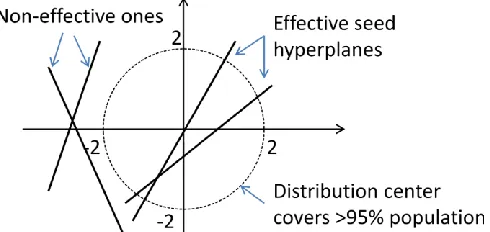
The basic idea is to find the hyperplanes that shatter around the center of the dataset. Because the OPE transformed dimensions have normal distributions, we can imagine the records projected to these d dimensions are distributed in an ellipsoid. Figure 2 shows the two-dimension, with each dimension in standard normal distribution. The majority of the records is inside the hyper-sphere of radius γ = 2 with the center at (0 ,0).
Fig. 2. Effective hyperplanes shatter around the distribution center.
Thus, to shatter in the major population, we need to have the distance between the center o and
(5)
Where kwk is the length of the vector w, and |b| is the absolute value of b. γ can be set to the minimum dimensional standard deviation. To satisfy this condition, we can simply generate a unit-length random vector w, and then choose a random value b so that |wTo+b| < γ. Intuitively, the smaller the |wTo+b| value, the closer the hyperplane will be to the center. The client randomly generates a set of such hyperplanes as the pool and send to the cloud. Again, we will investigate how the pool size affects the learning result.
Cloud-side Processing
The cloud side will search the pool to find the best one that gives the lowest weighted error rate. Depending on the data distribution and the randomly generated candidates, there is a small probability that all the base learners in the pool give weighted error rates ∼ 50%. This probability will exponentially decrease with the increasing pool size. We will study the lower bounds of pool size for different datasets in experiments.
Seed-based Algorithms
In the pool based algorithms, the client needs to generate a set of randomly selected base classifiers, encode them, and send to the cloud. It might be costly, e.g., with hundreds of encoded classifiers. In the following, we consider reducing the client‟s work further by using the seed-based algorithms. The client will send a few randomly selected “seed classifiers”, and the cloud will generate a pool based on these seeds. The following algorithms depend on the linearity property of the query matrix Q.
Derived Decision Stumps (Derived DS)
The query matrices on the same dimension has the following linearity property.
Proposition 2
For half-space conditions on the same dimension, say Xi < a and Xi < b, a linear combination of the corresponding query matrix Qa and Qb: Qa + τ (Qb − Qa), τ ∈ R, is the query
matrix of some condition Xi < c on the same dimension.
Proof: For the condition Xi < a, we have the corresponding query y T Qay < 0 in the perturbed space, where Qa = (A−1) T uav T A−1 , u T a = (w, −E(a), 0) and v T = (0, . . . , v0, 1).
Similarly, Qb = (A−1) T ubv T A−1 , where u T b = (w, −E(b), 0). Therefore, it follows
Qa + τ (Qb − Qa) = (A −1) T (ua + τ (ub − ua))v T A −1 (6)
Where ua + τ (ub − ua) = (w, −E(a) − τ (E(a) − E(b)), 0). According to the definition of OPE, the value E (a) + τ (E (b)− E (a)) in the encrypted domain must correspond to a value in the original domain of Xi . Thus, Qa + τ (Qb − Qa) is the query matrix of some condition Xi < c.
Note that since τ can be any real value, E (a) + τ (E (b) − E(a)) can be any value in the OPE domain if E(b) 6= E(a). Therefore, with two randomly picked seed decision stumps on the same dimension, we can derive all decision stumps on the same dimension. However, not all of these decision stumps are effective for our use. Again, we hope the result will shatter around the center of the population (e.g., in the range (µ−2σ, µ+2σ) for the normalized data). We can achieve this goal by setting the seeds around the bounds [−γ, γ] on the OPE domain, where γ can be some value in (0, σ) and τ in the range (0, 1). With such a setting, we have |E(a) + τ (E(b) − E(a))| ≤ |(1 − τ )E(a)| + |τE(b)| < 2σ to shatter around the center of the population.
Derived Random Linear Classifier (Drived
LC)
The linearity property of query matrices can be extended to general linear classifiers on the OPE space.
Proposition 3
Assume a set of query matrices {Qi,i = 1..m} encode the general linear functions
OPE space, respectively. Then, ,
where τi ∈ R, represents a valid general linear function in the OPE space.
Proof: Similarly, we have =
. Apparently, is a valid
parameter vector for a general linear function in the OPE space.
Two key problems are to be addressed. First, we want the generated hyperplane to shatter around the major population. For simplicity of presentation, we assume all the dimensions have the center on 0. As we have discussed, the condition | Pm i=1 τibi |/k Pm i=1 τiwik < γ should be satisfied. However, k Pm i=1 τiwik can be a very small value close to 0, which dissatisfies the condition. Second, the random combination Pm i=1 τiwi represents the direction of the generated hyperplane, which should be able to cover as many possible directions as possible. We have the following result to address these problems.
Proposition 4
Let {wi , i = 1..d} be the random orthonormal vectors and P (τ1, . . . , τd) be a random unit vector, i.e., d i=1 τ 2 i = 1, and |bi | < γ/d. This condition is satisfied.
Proof: The proof follows the logic that if 1 and |Pmi=1 τibi| < γ then the
condition is satisfied. Let R be an orthonormal matrix, i.e., RT R = I. {wi} can be considered as the rotational transformation of the standard basis {ei , i = 1..d}: wi = Rei , where all elements of ei are 0 except for the i-th set to 1. Also, the transformation Rw for any vector w preserves the length of w, i.e., kRwk = kwk. Therefore, k Pd i=1 τiwik = k Pd i=1 Rτieik = k Pd i=1 q τieik = Pd i=1 τ 2 i = 1. Meanwhile, since |τi | ≤ 1, if |bi | < γ/d we have | Pd i=1 τibi | ≤ Pd i=1 |τi ||bi | ≤ γ. It is also straightforward to prove that any unit vector w can be represented with the above combination method Pd i=1 τiwi , where Pd i=1 τ 2 i = 1. It implies that this combination method can generate hyperplanes in any direction. Note that the d random orthogonal vectors {wi} can be easily obtained by applying QR decomposition of a random invertible d×d matrix. A random unit vector τ can be obtained from a random vector r by τ ← r/krk. Thus, it is easy for both the client to generate the seed vectors
and the cloud to generate the random combinations.
Cloud-side Processing
The cloud side will randomly generate a batch derived decision stumps or linear classifiers to find the best one. Similar to the pool based algorithms, the problem is the appropriate number of random trials. We will investigate this problem in experiments.
Cost analysis
and O (d (d+ 2)2) for linear classifiers. Thus, if the pool has a size of p, the first option has the total cloud side cost O (k (d + 2)2N), while the second O (kp (d + 2)2N).
Confidentiality analysis
Confidentiality guarantee consists of several parts: the confidentiality of perturbed data in the cloud, the confidentiality of queries and the learning process, and the confidentiality of generated models. We discuss them separately in the following.
Data confidentiality
Data confidentiality has been discussed in our paper on the RASP approach for outsourced databases. We include the key points here to make the paper self-contained. According to the threat model, the attacker may know only the perturbed data, i.e., the first level of prior knowledge, or the distribution of each dimension, i.e., the second level, which corresponds to the brute-force attack, and the ICA attack, respectively.
To conveniently represent the complexity of attacks, we assume each value in the vector or matrix is encoded with or converted to n-bit integers. Let the perturbed vector y be drawn from a random variable Y, and the original vector x be drawn from a random variable X. The corresponding matrices are X and Y .
Brute-Force Attack
This attack will examine each possible original matrix X according to the known Y . We show that this process is computationally intractable. The goal is to show the number of the valid X dataset in terms of a known perturbed dataset Y . Below we discuss a simplified version that contains no OPE component - the OPE version has at least the same level of security.
Proposition 5
For a known perturbed dataset Y , there exists O(2(d+1)(d+2)n) candidate X datasets in the original space to be examined.
Proof: For a given perturbation Y = AZ, where Z is X with the two extended dimensions, we have A −1Y = Z. Let B = A −1 and B
d+1 represent the (d + 1)-th row of A−1. We have B d+1Y = [1,...,1], i.e., the
appended (d + 1)- th row of Z. Keeping B d+1 unchanged, we randomly generate other rows of B for a candidate Bˆ. The result Zˆ = BPˆ is a validate estimate of Z if Bˆ is invertible. Thus, the number of candidate X is the number of invertible Bˆ.
The total number of Bˆ including non-invertible ones is 2 (d+1)(d+2)n. Based on the theory of invertible random matrix, the probability of generating a non-invertible random matrix is less than exp −c(d+2) for some constant c. Thus, there are about (1 − exp −c(d+2))2(d+1)(d+2)n invertible Bˆ. Correspondingly, there are a same number of candidate X.
Thus, examining all possible X is computationally intractable, and the brute-force attack is impractical.
ICA Attack
With the known distributional information, the attacker can do more on estimating the original data than simple. The known most relevant method is called Independent Component Analysis (ICA). For a multiplicative perturbation Y = AX, the fundamental method, is to find an optimal projection, wY , where w is a d+2 dimension row vector, to result in a row vector with its value distribution close to that of one original attribute. This goal is approximately achieved by examining the non-gaussianity2 characteristics of the original distribution - finding the projections by maximizing the non-gaussianity of the result wY. The non-gaussianity of the original attributions is crucial because any projection of a multidimensional normal distribution is still a normal distribution, which leaves no clue for recovery.
To simplify the proof, we assume the original dimensions are independent. We have the following result.
Proposition 6
There are O (2dn) candidate projection vectors, w, that lead to the same level of non-gaussianity.
we consider grouping all the independent d + 1 dimensions together as the submatrix Z1. Z1 contains the sample vectors from a d + 1-dimensional normal distribution N (µ, Σ), where µ is the mean and Σ is the covariance matrix. Thus, the RASP transformation can be represented as Y = (A1, A2) (Z T 1, 1)T, where A1 is the first d + 1 columns of the A matrix, A2 is the last column, and 1 is the added constant row of 1. It follows Y = A1Z + A2 · 1. According to the basic property of multidimensional normal distribution, A1Z contains samples from the multidimensional normal distribution N (A1µ, A1ΣAT 1). A2 · 1 simply adds a constant to each row vector (i.e., a dimension) of A1Z, which does not change the dimensional distribution. Therefore, Y has a multidimensional normal distribution.
It immediately follows that any projection wY will not change the Gaussianity of the result, and there are O (2dn) such candidates of w.
Thus, enumerating all possible projections and analyzing each is computationally impractical. It shows that any ICAstyle estimation that depends on Gaussianity is equally ineffective to the RASP perturbation. In addition to ICA, Principal Component Analysis (PCA) based attack is another possible distributional attack, which, however, depends on the preservation of covariance matrix. Because the covariance matrix is not preserved in RASP perturbation, the PCA attack cannot be used on RASP perturbed data. It is unknown whether there are other distributional methods for approximately separating X or A from the perturbed data Y, which will be studied in the ongoing work.
Query and Process Privacy
Queries in the proposed algorithms consist of two parts: the original queries generated by the client, and the derived queries by the cloud using the seed-based query derivation algorithms, for which we need to check whether the derivation algorithm gives additional information. According to the threat model, the attacker does not have any additional prior knowledge about queries except for the known matrix Q. Now, the task is to find the decomposition of a query matrix Q = (A−1 ) T uvT A−1 to figure out any information about A−1 and u (since v is constant, we consider it is known
by the public). We show that a stronger attack with additional knowledge of u is still computationally intractable.
Proposition 7
With known u, there are about O (2(d−1)(d+2)n) valid guesses of A that result in the same query matrix Q.
Proof: Without loss of generality, we can assume that Q encodes a condition Xi < a. Let ri be the i-th row of A−1 . Q is represented as (ri − E(a)rd+1) T (rd+2 − v0rd+1). Note that Q is only determined by the three rows of the matrix A−1 . The remaining d − 1 rows are free to choose, leading to 2 (d−1)(d+2)n valid candidates of A−1 , among which O(2(d−1)(d+2)n) are invertible .
This shows a lower bound of the difficulty in attacking the Q matrix without any additional information. The next problem is whether the cloud-side algorithms will breach additional information. Obviously, since all the algorithms either simply search the pool or use purely random combinations of existing query matrices, there is no additional information is leaked.
Model confidentiality
As we have discussed in Section 4, model confidentiality is defined as c (f, p) = min{c (f, p, Di)}, where f is the learned model, p are the unknown parameters, Di is the p distribution estimated by an attacker, c(f, p, Di) is the model utility reduction under the attack. The smaller the reduction, the more effective the attack.
For classification modeling, we use the accuracy on the testing data T as the model utility. In a boosting model f(x) = Pn i=1 αihi(x), the model parameters consist of n, {αi}, and the parameters in hi(x). If hi(x) are decision stumps, the parameters include the selected dimension, the splitting value, and the direction: Xj < a or Xj ≥ a. For linear classifiers on the OPE space, w, b, and the direction: w tx + b < 0 or w tx + b ≥ 0 are the parameters of the base model.
parameters. As we have discussed, under our security assumption the only known attack on the query matrix is the brute-force attack, which, however, is computationally intractable. Since hi(x) (especially for smaller i) are significant to the model, we expect the model confidentiality is preserved well. In experiments, we will further explore the concept of model confidentiality
Evaluation
The previous sections have addressed several major aspects: the cloud-client algorithms, the
client-side cost analysis, and the confidentiality analysis. The experiments will study how the cloud-client algorithms perform in terms of different settings that may also involve the trade-off between model quality and client-side costs. Specifically, we will show the scalability of our approach with client-side computation and communication costs on real datasets. We will conduct a set of experiments to understand which of the four private learning methods is the best in terms of costs and model quality. We will evaluate model confidentiality with the proposed method.
Table: Datasets for experiments.
Dataset Records Dimensions Link
German Credit 1000 20 https://goo.gl/lVy34O
Ozone Days 2536 73 https://goo.gl/Si6aDh
Spam base 4601 57 https://goo.gl/WPyXTi
Bank Marketing 45211 17 https://goo.gl/vvgj3M
Twitter Buzz 140000 77 https://goo.gl/Yfy80u
Experiment setup
Datasets
For easier validation and reproducibility of our results, we use a set of public datasets from UCI machine learning repository for evaluation, each of which has only two classes. These datasets have been widely applied in various classification modelling and evaluation. These datasets have been widely applied in classification modelling and evaluation. Table 1 lists statistics of the datasets. They cover different scales and dimensions to make the results more representative. In pre-processing, each dimension of the datasets is normalized with the transformation , Where is the mean
and is the variance of the dimension j.
Implementation
We implement the perturbation methods based on the algorithms in the corresponding papers. The RASP-Boost framework is implemented based on the A da Boost algorithm. The four learning algorithms are implemented as plugins to the framework. All these implementations use C++ and are thoroughly tested on a Ubuntu Linux server. We also used the Sickest-Learn toolkit to
generate the AdaBoost baseline accuracy based on the original datasets for comparison.
CONCLUSION
single-dimensional method and the multi-resource method without skewness consideration. From the comparisons, we found that ignoring heterogeneity in the workloads led to huge wastage in resources. Specifically, by conducting simulation studies with three synthetic workloads and one cloud trace from google, it revealed that our proposed allocation
approach that is aware of heterogenous vms is able to significantly reduce the active pms in data centre, by 45% and 11% on average compared with single-dimensional and multi-resource schemes, respectively. We also showed that our solution maintained the allocation delay within the present target.
REFERENCES
[1]. A. Narayanan and V. Shmatikov, “Robust de-anonymization of large sparse datasets,” in Proceedings of the IEEE Symposium on Security and Privacy, 2008, pp. 111–125.
[2]. R. Agrawal and R. Srikant, “Privacy-preserving data mining,” in Proceedings of ACM SIGMOD Conference. Dallas, Texas: ACM, 2000. [3] B. C. M. Fung, K. Wang, R. Chen, and P. S. Yu, “Privacy-preserving data publishing: A survey of recent developments,” ACM Computing Survey, vol. 42, pp. 14:1–14:53, June 2010. [3]. C. Dwork, “Differential privacy,” in International Colloquium on Automata, Languages and Programming.
Springer, 2006.
[4]. H. Xu, S. Guo, and K. Chen, “Building confidential and efficient query
[5]. services in the cloud with rasp data perturbation,” IEEE Transactions on Knowledge and Data Engineering, vol. 26, no. 2, 2014.
[6]. Z. Brakerski, C. Gentry, and V. Vaikuntanathan, “(leveled) fully homomorphic encryption without bootstrapping,” in Proceedings of the 3rd Innovations in Theoretical Computer Science Conference, ser. ITCS ‟12. New York, NY, USA: ACM, 2012, pp. 309–325.
[7]. Y. Huang, D. Evans, J. Katz, and L. Malka, “Faster secure two-party computation using garbled circuits,” in Proceedings of the 20th USENIX Conference on Security, ser. SEC‟11. Berkeley, CA, USA: USENIX Association, 2011, pp. 35–35.
[8]. B. Schneier, “Homomorphic encryption breakthrough,” http://tinyurl.com/nlzv4w, 2009.
[9]. V. Nikolaenko, S. Ioannidis, U. Weinsberg, M. Joye, N. Taft, and D. Boneh, “Privacy-preserving matrix factorization,” in Proceedings of the 2013 ACM SIGSAC conference on Computer and communications security. New York, NY, USA: ACM, 2013, pp. 801–812.
[10].K. Chen and L. Liu, “Geometric data perturbation for outsourced data mining,” Knowledge and Information Systems, vol. 29, no. 3, 2011.
[11].K. Liu, H. Kargupta, and J. Ryan, “Random projection-based multiplicative data perturbation for privacy preserving distributed data mining,” IEEE Transactions on Knowledge and Data Engineering (TKDE), vol. 18, no. 1, pp. 92–106, 2006.
[12].Y. Lindell and B. Pinkas, “Privacy preserving data mining,” Journal of Cryptology, vol. 15, no. 3, pp. 177– 206, 2000.
[13].K. Liu, C. Giannella, and H. Kargupta, “An attacker‟s view of distance preserving maps for privacy preserving data mining,” in Proceedings of PKDD, Berlin, Germany, September 2006.
[14].C. Gentry, “Fully homomorphic encryption using ideal lattices,” in Annual ACM Symposium on Theory of Computing. New York, NY, USA: ACM, 2009, pp. 169–178.
[15].M. Cooney, “Ibm touts encryption innovation,” http://tinyurl.com/d7xpkuk, 2009.
[16].T. Graepel, K. Lauter, and M. Naehrig, “Ml confidential: Machine learning on encrypted data,” in Proceedings of the 15th International Conference on Information Security and Cryptology, ser. ICISC‟12. Berlin, Heidelberg: Springer-Verlag, 2013, pp. 1–21.
[17].R. Bost, R. A. Popa, S. Tu, and S. Goldwasser, “Machine learning classification over encrypted data,” in 22nd Annual Network and Distributed System Security Symposium, NDSS 2015, San Diego, California, USA, February 8-11, 2014, 2015.
of ACM SIGMOD Conference, 2004.
[19].H. Hacigumus, B. Iyer, C. Li, and S. Mehrotra, “Executing sql over encrypted data in the database-service-provider model,” in Proceedings of ACM SIGMOD Conference, 2002.