Two point fuzzy boundary value problem with eigenvalue parameter contained in the boundary condition

https://doi.org/10.26637/MJM0604/0010

Two point fuzzy boundary value problem with

eigenvalue parameter contained in the boundary

condition

Tahir Ceylan

* and Nihat Altını¸sık

Abstract

In this article two point fuzzy boundary value problem is defined under the approach generalized Hukuhara differentiability (gH-differentiability). We research the solution method of the fuzzy boundary problem with the

basic solutionsΦb(x,λ)andχb(x,λ)which are defined by the special procuder. We give operator-theoretical

for-mulation, construct fundamental solutions and investigate some properties of the eigenvalues and corresponding eigenfunctions of the considered fuzzy problem. Then results of the proposed method are illustrated with a numerical example.

Keywords

gH-derivative, eigenvalue, fuzzy eigenfunction, fuzzy Hilbert Space.

AMS Subject Classification

03E72, 34A07, 65L05.

1_{Department of Mathematics, Faculty of Arts and Sciences, Sinop University, 57000, Sinop, Turkey.}

2_{Department of Mathematics, Faculty of Arts and Sciences, Ondokuz Mayıs University, 55139, Kurupelit, Samsun, Turkey.} *Corresponding author:1_{[email protected];} 2_{[email protected]}

Article History: Received21August2018; Accepted26October2018 c2018 MJM.

Contents

1 Introduction. . . 766 2 Preliminaries. . . 767 3 Operator-Theoretic Formulation of the Problem. . 769 4 Solution Method of the Fuzzy Problem. . . 769 5 Conclusion. . . 772

References. . . 772

1. Introduction

In this paper we consider the two point fuzzy boundary value problem

L=−d 2

dt2

L_bu=λ_bu, t∈[a,b] (1.1)

which satisfy the conditions

b

a1ub(a) =ab2bu

0_{(a) (1.2)}

b

b1u_b(b) =λbb2u_b0(b) (1.3)

wherea1_b,a2_b,bb1,bb2are nonnegative triangular fuzzy numbers,

λ>0 reel number,_ba1+ba26=0,bb1+bb26=0 andub(t)fuzzy function.

goes [3]. So here we use gH-difference and gH-derivative to solve FDE under much less restrictive conditions [11].

The paper is organized as follows; section 2 introduces the basic concept of fuzzy function spaces, fuzzy Hilbert spaces and fuzzy gH- derivative. In section 3, we define operator formulation of the problem in the adequate fuzzy Hilbert spaces. In section 4, we give a numerical example. In section 5, the results are stated gained through the study of the paper.

2. Preliminaries

In this section, we give some concepts and results besides the essential notations which will be used throughout the paper.

Letu_bbe a fuzzy subset onR, i.e. a mappingub:R→[0,1] associating with each real numbertits grade of membership b

u(t).

In this paper, the concept of fuzzy real numbers (fuzzy intervals) is considered in the sense of Xiaoand Zhu which is defined below:

Definition 2.1. [2]. A fuzzy subset_bu onRis called a fuzzy

real number (fuzzy intervals), whoseα−cut set is denoted by

[u_b]α, i.e.,[bu]α={t:ub(t)≥α}, if it satisfies two axioms:

(N1) There exists r∈Rsuch thatub(r) =1.

(N2) For all0<α≤1, there exist real numbers−∞<u−_α ≤ u+_α <+∞such that[u_b]α is equal to the closed interval

[u−_α,u+_α].

The set of all fuzzy real numbers (fuzzy intervals) is de-noted byF(_R).FK(_R), the family of fuzzy sets of_Rwhose

α−cuts are nonempty compact subsets ofR. Ifub∈F(R) and_bu(t) =0 whenevert<0, then_buis called a non-negative fuzzy real number andF+(R)denotes the set of all non-negative fuzzy real numbers. For all_bu∈F+₍

R)and each

α∈(0,1], real numberu−α is positive.

The fuzzy real number_br∈F(R)defined by

b

r(t) =

1,t=r

0, t6=r,

it follows that_Rcan be embedded inF(_R), that is if_br∈

(−∞,∞), then_br∈F(R)satisfiesrb(t) =b0(t−r)andα−cut of_bris given by[_br]α= [r,r],α∈(0,1].

Definition 2.2. [3] An arbitrary fuzzy number in the para-metric form is represented by an ordered pair of functions

(u_α−,u_α+),0≤α≤1, which satisfy the following requirements

(i) u_α−is bounded non-decreasing left continuous function on(0,1]and right- continuous forα=0,

(ii) u_α+is bounded non-increasing left continuous function on(0,1]and right- continuous forα=0,

(iii) u_α−≤u_α+,0≤α≤1.

Definition 2.3. [13] Let[aα_bα_{],0<α≤1, be a given family}

of non-empty intervals. Assume that

(a) [aα1_,bα1_]⊃[aα2_,bα2_{]for all0<α} 1≤α2,

(b)

lim

k→−∞a

αk_,lim

k→∞b

αk

= [aα_,bα_{]whenever{αk}is an}

in-creasing sequence in(0,1]converging toα,

(c) −∞<aα_≤bα_{<+∞, for allα∈(0,1].}

Then the family[aα_,bα_{]represents the}

α−cut sets of a

fuzzy real numberu_b∈F(R).Conversely if[aα,bα],0<α≤

1, are theα−cut sets of a fuzzy numberbu∈F(R), then the conditions (a), (b) and (c) are satisfied.

Definition 2.4. [3] For u,_bv_b∈F(R), andλ ∈R, the sum b

u⊕_bv and the productλu are defined by for all_b α∈[0,1]

[u_b⊕_bv]α _{= [}

b

u]α_{+ [}

b

v]α_={x+y:x∈[

b

u]α_,y∈[

b

v]α_},

[λ_bu]α = λ[u_b]α={λx:x∈[u_b]α}.

Defined:F(R)×F(R)→R+∪ {0}by the equation

d(u,_bv_b) = sup 0<α≤1

{max[|u_α−−v_α−|,|u+

α −v

+

α|]}

where[_bu]α_{= [u}− α,u

+

α],[bv]

α_{= [v}− α,v

+

α].

LetT ⊂Rbe an interval. We denote by theF(C(T;Rn)) space of all continuous fuzzy functions onT. For _bu, _bv∈ F(C(T;Rn)), define a metric

D∗(u,_bbv) =sup t∈T

d(u_b(t),v_b(t)).

From [3],F(C(T;_Rn_),D∗_{)is a complete metric space.}

A fuzzy functionFb:T →F(R)is measurable if for all

α∈[0,1], the set valued mappingFα:T →FK(R)defined

byeFα(t) =

h b

F(t)iα is measurable.

Let L1(T;R) denote the space of Lebesque integrable functions. We denote byeS1_Fthe set of all Lebesque integrable selections ofFα:T→FK(R), that is

S1_F=

f ∈L1(T;_R): f(t)∈Fα(t) a.e (2.1)

A fuzzy functionFb:T →F(R)is integrably bounded if there exists an integrable functionhsuch thatkxk ≤h(t) for allx∈F0(t). A measurable and integrably bounded fuzzy

functionsFα:T →FK(R)is said to be integrable overT if

there existsFb∈F(R)such that

Z

T

Fα(t)dt=

Z

T

f(t)dt: f∈S1_F

,

for allα∈[0,1][7].

kfk_Lp

T=

( (R

T|f(t)| p

dt)1p_{, 1≤p<∞}

inf_µ(T

0)=0supt∈T−T0|f(t)|, p=∞ )

,

whereµ(T)is the Lebesque measure onT andT0⊂T. Let Lp(T;R)be the Banach space of all measurable functions

f :T→RwithkfkL_Tp <∞. ByF(Lp(T;R)), 1≤p<∞, it

is denoted the space of all functionsu_b:T →F(_R)such that the functiont→d(u_b(t),b0)belong toLp(T;R+). Then

dp(bu,bv) = Z 1

0

(dH([u_b]α_,[

b

v]α₎₎p_d

α

1_p

(2.2)

is ametric onF(Lp(T;R)), and for 1≤p<∞

d∞(u,_bbv) =d(u,_bbv) = sup

0≤α<1

dH([u_b]α_,[

b

v]α_{) (2.3)}

is a metric onF(L∞_(T;

R))[7]. So forp=2, letL2_(T;

R)be the Banach space of all mea-surable functionsf:T→Rwithkfk_L2

T<∞. ByF L

2_(T;

R), we denote the space of all square-integrable fuzzy functions

b

u:T →F(R)such that the functiont→d(bu(t),b0)belong toL2(T;R+). Then from(2.2)

d2(u,_bv_b) = Z 1

0

(dH([_bu]α_,[

b

v]α₎₎2_dα

1₂

is a metric onF L2(T;R), forp=2.

Definition 2.5. [9] Let X be a vector space overR. A

Felbin-fuzzy inner product on X is a mappingh., .i:X×X→F+₍ R)

such that for all vectors x,y,z∈X and all r∈_R, have

(FIP1) hx+y,zi=hx,zi ⊕ hy,zi

(FIP2) hrx,yi=|r| hx,yi

(FIP3) hx,yi=hy,xi

(FIP4) x6=0⇒ hx,xi(t) =0, for all t<0 (FIP5) hx,xi=0if and only if x=0.

Remark 2.6. Condition (FIP4) in the above definition is equivalent to the condition for all(06=)x∈X hx,xi_α−>0, for eachα∈(0,1]where[hx,xi]α=hx,xi−_αhx,xi+_αsee in [9].The vector space X equipped with a Felbin-fuzzy inner product is called a Felbin-fuzzy inner space. A Felbin-fuzzy inner product on X defines a fuzzy number

kxk=p2

hx,xi, for all x∈X. (2.4)

A fuzzy Hilbert space is a complete Felbin-fuzzy inner product space with the fuzzy norm defined by(2.4).

Example 2.7. Consider the lineer space L2([0,1];R)of all

square-integrable functions. Define

hf,gi(t) =sup

α∈(0,1]

t∈

Z 1

0

f_α−g−_αdx,

Z 1

0

f_α+g+_αdx

(2.5)

for f,g∈L2[0,1]such thatFb,Gb∈F L2([0,1];R)

. It can be showed thathf,giis Felbin-fuzzy inner product space on L2[0,1]andα-cut set ofhf,giis given bye

[hf,gi]_α=hf,gi_α−,hf,gi_α+

= Z 1

0

f_α−(x)g−_α(x)dx,

Z 1

0

f_α+(x)g+_α(x)dx

(2.6)

for allα∈[0,1]. From theorem 6 of [8], it is clear thathf,gi is a fuzzy real number. So L2([0,1];R)is a fuzzy Hilbert

space.

Definition 2.8. [10]. Let _bu,_bv∈F(R). If there exist wb∈

F(R)such thatub=bv⊕w,b thenw is called the Hukuharab

difference ofu and_{b b}v and it is denoted byu_b hbv. Ifub hvb

exists, itsα−cuts are

[u_b Hbv]

α₌

u_α−−v_α−,u_α+−v_α+

for allα∈[0,1].

Definition 2.9. The generalized Hukuhara difference of two fuzzy numbersu,_bbv∈F(R)is defined as follows

[u_b gHvb] =wb⇔

(i) u_b=_bv⊕w_b or(ii) _bv=u_b⊕(−1)w._b

In terms ofα-cuts we have

[u_b gHvb]

α ₌

min

u_α−−v_α−,u_α+−v+

α ,

maxu_α−−v_α−,u_α+−v_α+

and if the H -difference exists, thenu_b hbv=bu gHv; theb

conditions for the existence ofw_b=_bu gHbv∈F(R)are

case (i)

w_α−=u_α−−v_α−and w_α+=u_α+−v+

α,∀α∈[0,1]

with w_α−increasing, w_α+decreasing,w_α−≤w_α+

case (ii)

w_α−=u_α+−v+

α and w

+

α =u

−

α −v

−

α,∀α∈[0,1]

with w_α−increasing, w_α+decreasing,w_α−≤w_α+. It is easy to show that (i) and (ii) are both valid if and only if w is a crisp number [11].

Remark 2.10. Throughout the rest of this paper, we assume thatu_b gHbv∈F(R)andα-cut representation of fuzzy

val-ued function bf :(a,b)→F(R)is expressed by h

b

f(t)iα= [(f_α−) (t),(f_α+) (t)], t∈[a,b]for eachα∈[0,1].

Definition 2.11. [11] Let t0∈(a,b)and h be such that t0+

h∈(a,b), then the gH-derivative of a function bf :(a,b)→

F(R)at t0is defined as

b

f_gH0 (t0) =lim h→0

f(t0+h) gH f(t0)

h . (2.7)

If bf_gH0 (t0)∈F(R)satisfying(2.7)exists, we say that bf is

Definition 2.12. [11] Let bf :[a,b]→F(_R)and t0∈(a,b)

with f_α−(t)and f_α+(t)both differentiable at t0. We say that

- bf is[(i)−gH]-differentiable at t0if

h b

f_gH0 (t0)

iα

=h f_α−0(t), f_α+0(t)i (2.8)

- bf is[(ii)−gH]-differentiable at t0if

h b

f_gH0 (t0)

iα

=h f_α+0(t), f_α−0(t)i (2.9)

for allα∈[0,1].

Definition 2.13. The second generalized Hukuhara derivative of a fuzzy function bf :[a,b]→F(_R)at t0is defined as

b

f_gH00 (t0) =lim

h→0

b

f0(t0+h) gHbf0(t0)

h .

ifbf_gH00 (t0)∈F(R), we say thatbf_gH0 (t)is generalized Hukuhara

derivative at t0.

Also we say that bf_gH0 (t)is[(i)−gH]−differentiable at t0

if

b

f_i00_.gH(t0,α) =

(f_α−)00(t0),(fα+)

00

(t0), if bf be[(i)−gH]

(f_α+)00(t0),(fα−)

00

(t0)

,if bf be[(ii)−gH]

for allα∈[0,1],and that bf_gH0 (t)is[(i)−gH]−differentiable

at t0if

b

f_ii00_.gH(t0,α) =

(f_α+)00(t0),(f_α−)00(t0)

, if bf be[(i)−gH]

(f_α−)00(t0),(fα+)

00

(t0), if bf be[(ii)−gH]

for allα∈[0,1][12].

3. Operator-Theoretic Formulation of the

Problem

Consider the(1.1)−(1.3)eigenvalue problem.

This is not the usual type of eigenvalue problem because the eigenvalue appears in the boundary conditions; so, we cannot putL=−d2

dt2 and consider problem as a special case ofLu_b=λu_bbecauseD, the domain ofL, depends uponλ. So we enlarge our definition ofL. To do this we formulate a theoretic approach to the problem.

From theorem 6 of [8], we define a fuzzy Hilbert space

b

H=L2([0,1];R)with a Felbin-fuzzy inner product

hf,gi = Z 1

0

f_α−(t)g−_α(t)dt+ (f1)−_α(g1)−_α,

Z 1

0

f_α+(t)g+_α(t)dt+ (f1)+_α(g1)+_α

where F ∈hFb iα

=

[f_α−(t),f_α+(t)]

(f1)−α,(f1)

+

α

⊂H and G∈

h b Gi α =

[g−_α(t),g+_α(t)]

(g1)−α,(g1)

+

α

⊂HandFb,Gb∈F+ L2([0,1];R)

such thatf_α−(t),f_α+(t),g−_α(t),g+_α(t)∈L2([0,1];R)and (f1)−α,(f1)

+

α,(g1)

−

α,(g1)

+

α ∈R.

Consider the space of two- component fuzzy vectorsFb∈ b

H,whose first component is a twice gH-differentiable fuzzy function bf(t)∈F+ L2([0,1];_R)

and whose second com-ponent is a fuzzy real number bf1∈F+(R). Here Fb, bf(x) and bf1are pozitive fuzzy numbers and theirα−cut sets are

respectively[F_α−,F_α+],[f_α−(t),f_α+(t)]and

(f1)−α,(f1)

+

α

. In this fuzzy Hilbert space we construct the lineer operator

A:Hb→Hbwith domain

D(A) =  

 b

f(t) b f1 b

f(t),bf0(t)fuzzy absolutely continuous (see [6]) in [0,1];

b

a1bf(a) =a2_b bf0(a), bf1=bb2bf0(b)  



which acts by the ruleAFb=A

b

f(t) b

f1

=A bf(t)

b

b2bf0(b) !

=

−bf00(t) b

b1bf(b) !

withFb= b f b f1

∈D(A).

Thus the problem(1.1)−(1.3)can be written in the form

AFb=λFb

whereFb= b f b f1

∈D(A).Then the eigenvalues and the

eigenfunctions of the problem(1.1)−(1.3)are defined as the eigenvalues and the first components of the corresponding eigenelements of the operatorA, respectively.

4. Solution Method of the Fuzzy Problem

In this section we concern with fuzzy eigenvalues and eigenfunctions of two-Point fuzzy boundary value problems with eigenvalue parameter contained in the boundary condi-tion. To do this, at first we need to use fuzzy derivatives. So here we use gH-difference and gH-derivative to solve fuzzy problem [11].

Definition 4.1. Let_bu:[a,b]⊂_R→F(_R)be a fuzzy function and[u_b(t,λ)]α= [u−_α(t,λ),u+_α(t,λ)]be theα−cut represen-tation of the fuzzy functionu_b(t)for all t∈[a,b]andα∈[0,1]. If the fuzzy differential equation(1.1)has the nontrivial solu-tions such that u−_α(t,λ)6=0, u+α(t,λ)6=0thenλis eigenvalue

of(1.1).

Consider the eigenvalues of the fuzzy boundary value problem(1.1)−(1.3). Using theα−cut sets and[i−gH ]-differentiability ofu_b,[ii−gH]-differentiability of_bu0; we get from(1.1)−(1.3)forλ =k2(k>0):

h

− u−_α00(t),− u+_α00(t)i=λu−α(t),u

+

α(t)

(a1)−α,(a1)

+

α u

−

α(a),u

+

α(a)

=

(a2)−α,(a2)

+

α

h

u−_α0

(a), u+_α0

(a)i (4.2)

(b1)−α,(b1)

+

α u

−

α(b),u

+

α(b)

= λ(b2)−_α,(b2)+_αh

u−_α0(b), u+_α0(b)i. (4.3)

Suppose that the two linearly independent solutions of

u00+λu=0 classic differential equation are u1(t,λ) and

u2(t,λ). Using these solutions the general solution of the

fuzzy differential equation(4.1)is

[_bu(t,λ)]α=u_α−(t,λ),u+_α(t,λ)

where

u−_α(t,λ) = C1(α,λ)u1(t,λ) +C2(α,λ)u2(t,λ) u+_α(t,λ) = C3(α,λ)u1(t,λ) +C4(α,λ)u2(t,λ).

LethΦb(x,λ) iα

be a solution which is satisfying

u−_α(a),u+_α(a) = (a2)−α,(a2)

+

α

h

u−_α0(a), u+_α0(a)i =

(a1)−_α,(a1)+_α

(4.4)

initial conditions of fuzzy differential equations(4.1). This solution can be expressed as

Φ−α(t,λ) =C11(α,λ)u1(t,λ) +C12(α,λ)u2(t,λ)

Φ+α(t,λ) =C13(α,λ)u1(t,λ) +C14(α,λ)u2(t,λ).

(4.5)

and we write(4.4)in(4.5)such that

Φ−_α(a,λ) =C11(α,λ)cos(ka) +C12(α,λ)sin(ka) = (a2)−_α (Φ−_α)0(a,λ) =C13(α,λ)cos(ka) +C14(α,λ)sin(ka) = (a1)−_α.

From the determinant of the coefficients matrix of the above linear system, we getC11(α,λ)andC12(α,λ)such that

C11 = (a2)−_αcos(ka)−(a1)−_αsin(ka)

k , C12 = (a2)−αsin(ka) + (a1)

−

α

cos(ka)

k .

Substituting thisC11andC12coefficients the above equations

in(4.5), the general solution is obtained as

Φ−_α(t,λ) =

(a2)−αcos(ka)−(a1)

−

α

sin(ka)

k

cos(kt)

+

(a2)−αsin(ka) + (a1)

−

α

cos(ka)

k

sin(kt).

(4.6)

Similarly we findΦ+α(t,λ)as

Φ+α(t,λ) =

(a2)+αcos(ka)−(a1)

+

α

sin(ka)

k

cos(kt)

+

(a2)+αsin(ka) + (a1)

+

α

cos(ka)

k

sin(kt).

(4.7)

Let[χb(x,λ)]

α

be a solution which is satisfying

u−_α(b),u+_α(b)

=

(b2)−_α,(b2)+_α

(4.8)

h

u−_α0(b), u+_α0(b)i = (b1)−α,(b1)

+

α

initial conditions of fuzzy differential equations(4.1). This solution can be expressed as

χα−(t,λ) =C21(α,λ)u1(t,λ) +C22(α,λ)u2(t,λ)

χα+(t,λ) =C23(α,λ)u1(t,λ) +C4(α,λ)u2(t,λ).

(4.9)

and we write(4.8)in(4.9)such that

χ_α−(a,λ) =C21(α,λ)cos(ka) +C22(α,λ)sin(ka) =k2(b2)−α

(χ_α−)0(a,λ) =C23(α,λ)cos(ka) +C24(α,λ)sin(ka) = (b1)−α

.

From the determinant of the coefficients matrix of the above linear system, we getC21(α,λ)andC22(α,λ)such that

C21 = =k2(b2)−αcos(kb)−(b1)

−

α

sin(kb)

k ,

C22 = k2(b2)−_αsin(kb) + (b1)−_αcos(kb)

k .

Substituting thisC21andC22coefficients the above equations in(4.9), the general solution is obtained as

χ_α−(t,λ) =

k2(b2)−_αcos(kb)−(b1)−_αsin(kb)

k

cos(kt)

+

k2(b2)−αsin(kb) + (b1)

−

α

cos(kb)

k

sin(kt).

(4.10)

χ_α+(t,λ) =

k2(b2)+αcos(kb)−(b1)

+

α

sin(kb)

k

cos(kt)

+

k2(b2)+_αsin(kb) + (b1)+_α cos(kb)

k

sin(kt).

(4.11)

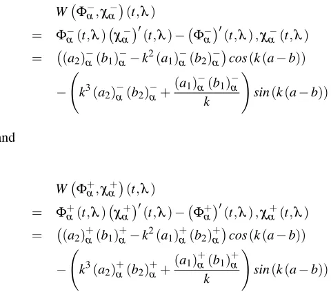
Then from(4.6)−(4.7)and(4.10)−(4.11)we find

W(Φ−_α,χ_α−) (t,λ)andW(Φ+_α,χ_α+) (t,λ)Wronskian functions as

W Φ−_α,χ_α−(t,λ)

= Φ−_α(t,λ) χ_α−0(t,λ)− Φ−_α0(t,λ),χ_α−(t,λ)

= (a2)−α(b1)

−

α−k

2_(a 1)−α(b2)

−

α

cos(k(a−b))

− k3(a2)−_α(b2)−_α+(a1)

−

α(b1)

−

α

k

!

sin(k(a−b))

and

W Φ+_α,χ_α+(t,λ)

= Φ+_α(t,λ) χ_α+0(t,λ)− Φ+_α0(t,λ),χ_α+(t,λ)

= (a2)+α(b1)

+

α−k

2_(a 1)+α(b2)

+

α

cos(k(a−b))

− k3(a2)+_α(b2)+_α+(a1) +

α(b1)

+

α

k

!

sin(k(a−b))

Theorem 4.2. The Wronskian functions W(Φ−_α,χ_α−) (t,λ) and W(Φ+_α,χ_α+) (t,λ)are independent of variable t for t∈

[a,b], where functionsΦ−_α,χ_α−,Φ+_α,χ_α+are the solution of the fuzzy boundary value problem(1.1)−(1.3)and it is show that W_α−(λ) =W(Φ−_α,χ_α−) (t,λ)and W_α+(λ) =W(Φ_α+,χ_α+) (t,λ) for eachα∈[0,1][4].

Theorem 4.3. The eigenvalues of the fuzzy boundary value problem(1.1)−(1.3)are coincided zeros of the functions W_α−(λ)and Wα+(λ)[4].

Example 4.4. Consider the two point fuzzy boundary problem

−_bu00 = λub (4.12)

b

u(0) = 0 (4.13)

h b

1i_bu(1) = λu_b0(1) (4.14)

where[1]α _{= [α,2−α]}

,λ =k2(k>0)and_bu(t)is[i−gH] -differentiable andu_b0(t)is[ii−gH]-differentiable fuzzy func-tions.

LethΦb(t,λ) iα

be the solution which is satisfying

u−_α(0),u+_α(0) =0

initial condition of fuzzy differential equations(4.12). Then we findhΦb(t,k)

iα

as

h b

Φ(t,λ)

iα

=sin(kx). (4.15)

Similarly let[χ_b(t,λ)]αbe the solution which is satisfying

u−_α(1),u+_α(1)

= λ

h

u−_α0(1), u+_α0(1)i = [α,2−α]

initial conditions of fuzzy differential equations(4.12). Then we find[_bχ(t,λ)]α as

χα−(t,λ) =k

2_{cos(kt−k) +}α

ksin(kt−k)

χ_α+(t,λ) =k2cos(kt−k) +(2−α)

k sin(kt−k).

(4.16)

From theorem 4.3, , eigenvalues of the fuzzy problem(4.12)

-(4.14)are zeros of the functions W_α−(λ)and W_α+(λ). So we get

W_α−(λ) = αsink−k3cosk (4.17) W_α+(λ) = (2−α)sink−k3cosk. (4.18)

For eachα∈[0,1]if the k values satisfying(4.17)and(4.18) equations compute with Matlab Program, then an infinite number of eigenvalues such thatλn= (kn)2are obtained. So we show first four k values of(4.17)with k1,nin table 1 such that

Table 1. For W_α−(λ)k1,nvalues corresponding toα α∈[0,1] k1,0 k1,1 k1,2 k1,3

α=0 4.7124 7.8540 10.9956 14.1372 α=0.2 4.7105 7.8536 10.9954 14.1371 α=0.5 4.7176 7.8529 10.9952 14.1370 α=0.8 4.7147 7.8523 10.9950 14.1369 α=1 4.7028 7.8519 10.9948 14.1368 and first four k values of(4.18)with k1,nin table 1 such that

Table 2. For W_α+(λ)k2,nvalues corresponding toα α∈[0,1] k2,0 k2,1 k2,2 k2,3

α=0 4.6930 7.8498 10.9941 14.1364 α=0.2 4.6950 7.8503 10.9942 14.1365 α=0.5 4.6979 7.8509 10.9944 14.1366 α=0.8 4.7008 7.8515 10.9947 14.1367 α=1 4.7028 7.8519 10.9948 14.1368 For each kn values and α ∈[0,1] graphic of Wα−(λ)and

W_α+(λ)functions are given figures 1.

So if we write k1,nand k2,nvalues in(4.15)and(4.16) equations, thenhΦnb (t,λ)

iα

and[χn_b (t,λ)]αare

h b

Φn(t,λ)

iα

Figure 1.W_α−(λ),W_α+(λ)andW(λ)

(4.19)

and

[χbn(t,λ)]

α

= (χn)

−

α(t),(χn)

+

α(t)

=

(k1,n)2cos(k1,nt−k1,n) + α k1,n

sin(k1,nt−k1,n)

,

(k2,n)2cos(k2,nt−k2,n) +

(2−α) k2,n

sin(k2,nt−k2,n)

.

(4.20)

Then for all α ∈[0,1], (4.19) are eigenfunctions cor-responding to λ1,n= (k1,n)2 eigenvalues satisfying (4.17) equation and (4.20) are eigenfunctions corresponding to λ2,n= (k2,n)2eigenvalues satisfying(4.18)equation.

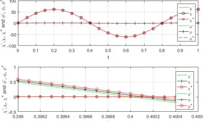
Consider that eigenvalues ofhΦnb (t,λ) iα

and[χn_b (t,λ)]α eigenfunctions depend onα−cut. So if we changeα,then this eigenvalues change and eigenfunctions corresponding toλ change. In particular, we select k1,1=7.8540in table 1 and k2,1=7.8498in table 2 forα =0. If we substitute this values respectively in(4.19) and(4.20), we have the following figures forbχandΦbfunctions.

Figure 2.χbEigenfunctions and fuzzy interval ofbχ

Figure 3.ΦbEigenfunctions and fuzzy interval ofΦb

Figure 4.α−cut ofχbandΦb Eigenfunctions

AlsoχbandΦbfunctions are given same grafic with figure

4.

In figure 2χα−,χ,χ

+

α functions and in figure 3Φ

−

α,Φ,Φ

+

α

functions are seem to have the same graphic. But because of eigenvalues have very close to each other, this eigenfunctions are different. AlsohΦnb (t,λ)

iα

and[χn_b (t,λ)]αeigenfunctions are fuzzy at certain intervals see figures.

5. Conclusion

Eigenvalues and eigenfunctions of the fuzzy boundary problem are introduced and examined by using generalized Hukuhara differentiability concept. In this problem, the eigen-value parameter is contained in the boundary condition atb. So we define lineer operator in fuzzy Hilbert space. To solve this problem, we use some initial value problems. Then we give a numerical example.

References

[1] _{Y. Chalco-Cano and H. Roman-Flores, Comparison}

[2] _{I. Sadeqi, F. Moradlou and M. Salehi, On Approximate}

cauchy equation in Felbin’s type fuzzy normed linear spaces,Iranian Journal of Fuzzy Systems, 10(2013), 51-63.

[3] _{P. Diamond and P. Kloeden, Metric Spaces of Fuzzy Sets:}

Theory and Applications, World Scientific, Singapore, 180, 1994.

[4] _{H. G. Çitil and N. Altını¸sık, On the eigenvalues and the}

eigenfunctions of the Sturm-Liouville fuzzy boundary value problem,J. Math. Comput. Sci., 7(2017), 786-805.

[5] _{A. Khastan and J. J. Nieto, A boundary value problem for}

second order differential equations,Nonlinear Analysis, 72(2010), 43-54.

[6] _{L. T. Gomes and L. C. Barros, ,Annual Meeting of the}

North American Fuzzy Information Processing Society (NAFIPS), 1, 2012.

[7] _{R. P. Agarwal, S. Arshad, D. O’Regan and V. Lupulescu,}

Fuzzy fractional integral equations under compactness type condition,Fractional Calculus and Applied Analysis, 4(2012), 572-589.

[8] _{B. Daraby, Z. Solimani and A. Rahimi, A note on fuzzy}

Hilbert spaces,Journal of Intelligent and Fuzzy Systems, 31(2016), 313-319.

[9] _{A. Hasankhani, A. Nazari and M. Saheli, Some properties}

of fuzzy Hilbert spaces and norm of operators,Iranian Journal of Fuzzy Systems, 7(2010), 129-157.

[10] _{L. M. Puri and D. Ralescu, Differential and fuzzy}

func-tions,J. Math. Anal. Appl., 91(1983), 552-558.

[11] _{B. Bede and L. Stefanini, Generalized}

differentiabil-ity of fuzzy-valued functions,Fuzzy Sets and Systems, 230(2012), 119-141.

[12] _{A. Armand and Z. Gouyandeh, Solving two-point fuzzy}

boundary problem using variational iteration method,

Communications on Advanced Computational Science with Applications, (2013), 1-10.

[13] _{O. Kaleva and S. Seikkala, On fuzzy metric spaces,Fuzzy}

Sets and Systems, 12(1984), 215-229.

[14] _{O. Kaleva, Fuzzy differetial equations,Fuzzy Sets and}

Systems, 24(1987), 301-317.

[15] _{T. Ceylan and N. Altını ¸Sık, Eigenvalue problem with}

fuzzy coefficients of boundary conditions, , Scholars Journal of Physics, Math. and Stat., 5(2018), 187-193.

? ? ? ? ? ? ? ? ? ISSN(P):2319−3786 Malaya Journal of Matematik