Xinhua et al. World Journal of Engineering Research and Technology
RESEARCH ON INDUSTRIAL ROBOT MOTOR MODEL WITH
MODEL REFERENCE ADAPTIVE SPEED SENSORLESS
ALGORITHM
Dr. Xinhua Yan*, Xinxing Yan and Kezhi Zhang
Nobot Intelligent Equipment (Shandong) Co., Ltd., Liaocheng, China 252000.
Article Received on 30/07/2018 Article Revised on 20/08/2018 Article Accepted on 10/09/2018
ABSTRACT
Aiming at the speed identification problem of induction motor without speed sensor vector control, a mathematical model based on asynchronous motor d-p axis is designed. Firstly, the position sensorless control system of asynchronous motor based on model reference adaptive method (MRAS) is established. Then, the
estimation error of position sensorless control system is analyzed, the feasibility of the system is proved. Simulation and experimental researching on the dynamic performance of the system show that the system has small speed fluctuation, accurate speed estimation, good system robustness and good dynamic and static characteristics.
KEYWORD: Asynchronous motor; Model reference adaptation; Speed sensorless. 1. INTRODUCTION
To achieve high-performance speed control, speed closed-loop control is employed, with the motor shaft which is installed a speed sensor.[1] But in actual systems, there are some restrictions on speed sensor installing. The main problem are as follows: firstly, the installation of speed sensor reduces the robustness and simplicity of the system;[2] secondly, the price of the high-precision speed sensor is generally more expensive, increasing the system cost;[3-4] meanwhile, the installation of the speed sensor will reduce the reliability of the system under some harsh conditions (such as high temperature, humidity, etc.),[5] finally, installation of the speed sensor has some difficulties. For example, once improperly installed, the speed sensor will become a source of failure for the system.[6] Therefore, to avoid these
World Journal of Engineering Research and Technology
WJERT
www.wjert.org
SJIF Impact Factor: 5.218*Corresponding Author Dr. Xinhua Yan
Nobot Intelligent
problems, people turned to study the motor speed identification method without speed sensor.[7-8] In recent years, this research has also become a hot issue in alternating current (AC) drive fields.
Foreign countries began research in this area in the 1970s. For the first time, the application of speed sensorless vector control was completed by R. Joetten in 1983,[9] which made a new step for the development of AC drive technology. In the following ten years, scholars at home and abroad have done a lot of work in this area. Then, many methods have been proposed, which can be roughly divided into follows: 1. dynamic speed estimator;[10] 2. model reference adaptation;[11-12] 3. PI regulator method-based;[13] 4. adaptive speed observer;[14] 5. rotor tooth harmonic method;[15] 6. high frequency injection method;[16] 7. artificial neural network method-based.[17]
2. Motor mathematical model
To improve the performance of the AC motor speed control system and understand the vector control technology in depth, the studying of the asynchronous motor mathematical model and the mastering of the relationship and inner relationship between voltage, current, flux linkage, electromagnetic torque, slip angular frequency and motor parameters are necessary. The mathematical model of the asynchronous motor is a high-order, nonlinear, and strongly coupled multivariable system. The following assumptions are usually made when studying the multivariable mathematical model of the asynchronous motor: the three-phase winding is symmetrical and the spatial harmonic is ignored; the magnetic circuit saturation is ignored; the self-inductance and mutual inductance of each winding are linear; the core loss is ignored.
2.1 Mathematical model of asynchronous motor in three-phase stationary coordinate system
(1) Voltage equation
A
A s A
B
B s B
C
C s C
d
u R i
dt d
u R i
dt d
u R i
dt
Three-phase rotor winding voltage equation a
a r a
b b r b
c c r c
d
u R i
dt d
u R i
dt d
u R i
dt (2)
(2) Flux equation Stator flux equation
=
=
=
A AA A AB B AC C Aa a Ab b Ac c
B BA A BB B BC C Ba a Bb b Bc c
C CA A CB B CC C Ca a Cb b Cc c
L i L i L i L i L i L i
L i L i L i L i L i L i
L i L i L i L i L i L i
(3)
Rotor flux equation
=
=
=
a aA A aB B aC C aa a ab b ac c
b bA A bB B bC C ba a bb b bc c
c cA A cB B cC C ca a cb b cc c
L i L i L i L i L i L i
L i L i L i L i L i L i
L i L i L i L i L i L i
(4)
(3) Torque equation
2
[( ) sin ( ) sin( )
3 4
( ) sin( )]
3
e n sr A a B b C c A a B b C c
A a B b C c
T p M i i i i i i i i i i i i
i i i i i i
(5)
(4) Equation of motion
e e L n d j T T p dt
(6)
In addition, in the static three-phase coordinate system, the stator resistance voltage drop is ignored, and the electromagnetic torque can be written as
2
2 2 2 2
1
3
2 [ ( ) ]
r s s
e n
r s ls lr
R V
T P
R L L
(7)
2.2 Mathematical model of asynchronous motor under the αβ axis of two-phase stationary coordinate system
(1) Stator voltage equation
s s s s
s s s s
u R i p
u R i p
(2) Rotor voltage equation
r r r r r r
r r r r r r
u R i p
u R i p
(9)
(3) Stator flux equation
s s s m r
s s s m r
L i L i
L i L i
(10)
(4) Rotor flux equation
r m s r r
s m s r r
L i L i
L i L i
(11)
(5) Electromagnetic torque equation
( )
e n m s r r s
T p L i i i i
(12)
(6) Equation of motion
= e L
n
j d
T T
p dt
(13)
whereris the rotor rotational angular velocity;Rsis the stator winding resistance;Lsis the
stator winding self-inductance;Lris the rotor winding self-inductance;Lmis the fixed rotor
winding mutual inductance;pnis the magnetic pole pair.
2.3 Mathematical model of asynchronous motor in d-q axis of two-phase rotating coordinate system
The mathematical model is written in the stator synchronous rotation d-q coordinate system by electric motor convention
(1) Stator voltage equation
ds s ds ds e qs
qs s qs qs e ds
u R i p
u R i p
(14)
(2) Rotor voltage model
dr r dr dr e qr
qr s qr qr e dr
u R i p
u R i p
(3) Stator flux equation ds s ds m dr
qs s qs m qr
L i L i
L i L i
(16)
(4) Rotor flux equation dr m ds r dr qr m qs r qr
L i L i
L i L i
(17)
(5) Electromagnetic torque equation
e n m qs dr qr ds
T p L i i i i (18)
whereRsandRrare stator and rotor resistance;LsandLrare stator and rotor equivalent
self-inductance;LlsandLlrare stator and rotor leakage;Lmis stator and rotor mutual
sense;uds,uqs,udranduqrare stator rotor voltage d and q axis components;ids,iqs,idrandiqrare stator rotor current d and q axis components; ds,qs,drandqrare stator rotor flux linkage d and q axis components; eis the motor synchronous angular velocity;ris the rotor electrical
angular velocity; sis the slip angular velocity;pnandpare number of pole pairs and
differential operator;Vsis the stator phase voltage amplitude.
Oriented by the rotor flux linkage, so that the direction of the rotor flux linkage is in the direction of the d-axis of the synchronous rotating coordinate system, thendr r,qr0,and bringing them into the equation (17)
r m ds dr
r
m
qr qs
r L i i
L L
i i
L
(19)
Since squirrel cage rotor internal short circuit, thenudr uqr 0, and bring it and (15) into (19)
s
m qs
r r L i T
(20)
r
1
m sd r
L i T p
(21)
Then taking (19) into (18) can be expressed
e
n m qs r r
p L
T i
L
(22)
For above, the dynamic changes ofisdis ignored under the steady state, thenpisd 0, and
equation (15) can be written as r L im sd
(23)
Bring (23) into (20) and (22)
s
qs
r ds i T i
(24)
2 e
m
n ds qs
r L
T P i i
L
(25)
3. Vector Controls
3.1 Vector control Coordinate transformation
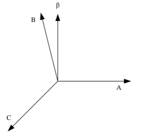
3.1.1 Three-phase and two-phase stationary coordinate system transformation (Clarke transform)
The stationary coordinate system transformation is a transformation between the three-phase stationary windings A, B, C and the two-phase stationary winding αβ, as shown in Figure 1
A B
C
β
Figure 1: Transformation between three-phase and two-phase stationary coordinate systems.
Phase motors have the same power and magnetomotive force and are completely equivalent in both electrical and magnetic.
The relationship from three-phase to two-phase transformation is:
1 1
1
-2 2 2
3 3 3
0
-2 2 a b c i i i i i (26)
The inverse transformation relationship is:
1 0
2 1 3
-3 2 2
1 3 - -2 2 a b c i i i i i (27)
3.1.2 Two-phase stationary and two-phase rotating coordinate system transformation (Park transformation)
The transformation between the two-phase stationary winding αβ and the two-phase rotating
d-q (MT) coordinate system, as shown in Figure 2. T β I i r i i M i M r
Figure 2: Two-phase stationary and two-phase rotating coordinate system transformation.
The relationship from two-phase stationary to two-phase rotating coordinate transformation is: cos sin sin cos d q i i i i
The relationship from two-phase rotating to two-phase stationary coordinate transformation is:
cos -sin sin cos
d q
i i
i i
(29)
3.2 Vector control principle
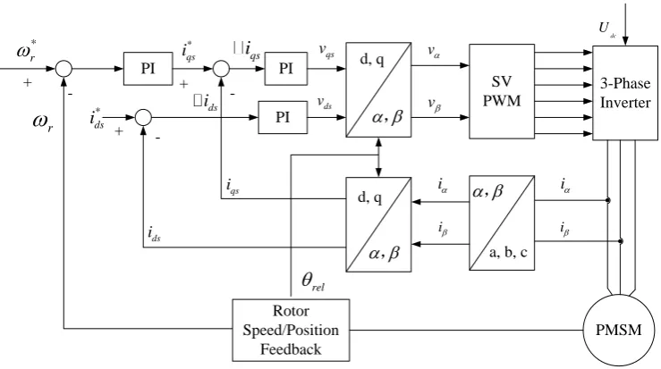
The control of the motor speed is basically achieved by controlling its torque. After the transformation from the three-phase stationary coordinate system ABC to the two-phase rotating coordinate system d-q, the control of the motor becomes simpler. According to the vector control principle diagram 3, the vector control system is mainly composed of the following parts:
(1) SVPWM module. Use advanced modulation algorithms to reduce current harmonics and increase DC bus voltage utilization;
(2) Current reading module. Measuring stator current through a precision resistor or current sensor;
(3) Rotor speed / position feedback module. Hall sensor or incremental photoelectric encoder is used to accurately obtain rotor position and angular velocity information, and sensorless detection algorithm can also be employed for measurement;
(4) PID control module;
(5) Clark, Park and anti-Park transformation modules.
PI PI d, q
SV PWM
3-Phase Inverter
PMSM d, q
a, b, c *
r
+ +
PI *
ds
i
+ - ,
,
,
Rotor Speed/Position
Feedback
*
qs i
r
-qs i
-ds
i
qs
i
ds
i
ds
v
qs v
i
i i
i
rel
v
v
dc
U
The vector control system can easily implement various control algorithms with the cooperation of the above modules. The implementation process can be divided into the following steps.
(1) The phase currentsiaandibmeasured by the current reading module are transformed from the three-phase stationary coordinate system to the two-phase stationary coordinate systemiand iby Clark transformation.
(2) iandiare combined with the rotor positionref and transformed from the two-phase stationary coordinate system to the two-phase rotating coordinate systemidsandiqsby Park transformation.
(3) The rotor speed/position feedback module compares the measured rotor angular velocityr with the reference speedr
and generates a quadrature reference currentiqsthrough the PI regulator;
(4) The AC and DC axis reference currents ids
and
qs
i are compared with the actual feedback of AC and DC axis currents ids and iqs, and the DC axis reference current ids
= 0 is taken, and then converted to voltages Vds and Vqs through the PI regulator.
(5) The voltages Vds and Vqs are combined with the detected rotor angular position ref to perform an inverse Park transformation to convert into two-phase stationary coordinate system voltages V and V.
(6) Voltages V and V are modulated by the SVPWM module into six-way switching
signals to control the switching of the three-phase inverter.
3.3 Model Reference Adaptive (MRAS)
Among the various methods, the model reference adaptive system is the most popular technique. If the speed estimation is attributed to reference identification, the model reference adaptive theory (MRAS) can be used to construct the identification speed system.
Reference Model
Adjustable mdoel
Identificatio n of law
r * X ^ X +
-Figure 4: Model reference adaptive schematic.
The model reference adaptive control principle can be signaled by the above block diagram 4. The main idea is to use the equation without the unknown parameter as the reference model and the equation containing the parameter to be estimated as the adjustable model. The two models have the same physical meaning output, using the error of the two model inputs constitutes a suitable adaptive law to adjust the parameters of the adjustable model in real time, in order to achieve the purpose of controlling the output tracking reference model.
MRAS is a parameter identification method based on stability design, which guarantees the asymptotic convergence of parameter estimation. However, the accuracy of MRAS's velocity observation depends on the correctness of the reference model and is affected by changes in the parameters of the reference model itself.
r r r
r
r r r
i
p A b
i
(30)
ˆ ˆ
ˆ ˆ
r r r
r
r
r r
i
p A b
i (31) where 1 - -1 -r r r A 1 ˆ - -ˆ 1 ˆ -r r r A
The speed identification formula can be defined as:
ˆ ˆ
ˆ ( ) ( ) ( )
ˆ ˆ ˆ ˆ
i
p r r r r r r
T K
K
s
4. Simulation results and analysis
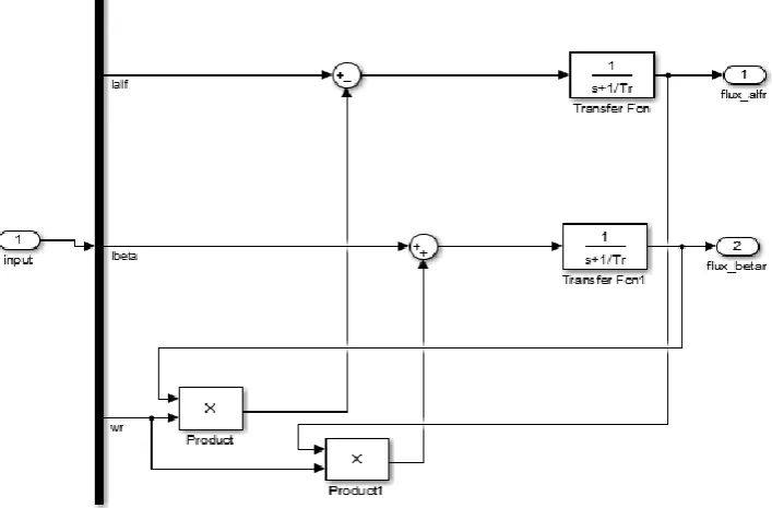
4.1 MRAS speed estimation module is built
Based on the above equation, the MRAS speed estimation module is constructed. Inverter DC bus voltage is 300 V, asynchronous motor (PMSM) parameters are set to: resistance R=0.9585Ω, stator d and q phase winding inductance Ld=Lq=5.25 mH, moment of inertia J=0.0006329 kg·m2, pole logarithm p=4. At time t=0, the load torque T=3N·m is applied to the motor, and the given speed is 600r/min; at t=0.1s, the load torque T=6N·m; at t=0.3s. The given speed is 1200r/min and the simulation time is 0.5s. The rotor flux observation model composed of the rotor can form a corresponding vector control system. The reference model module is built in MATLAB as shown in Figure. 5.
Figure 5: Model reference adaptive estimation module.
Because the relevant adjustments need to be made during the speed estimation process, the specific adjustment model is:
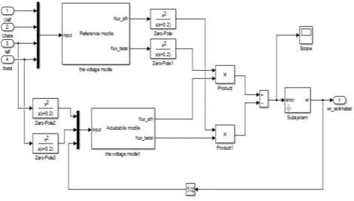
In summary, the adjustment module and the model reference adaptive module are integrated correspondingly, and finally packaged as the speed estimation module shown in Figure 7.
Figure 7: Speed estimation module.
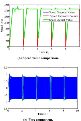
Through simulation analysis, the three-phase current waveform (Fig. 8(a)), the speed value comparison (Fig. (b)) and the flux linkage waveform (Fig. 8(c)) are obtained. It can be seen from the simulation results that after the motor starts with load, the speed rises rapidly to a given speed of 300r/s, and then a stable state occurs for a while. At the same time, the electromagnetic torque follows the load torque and the electromagnetic torque is quickly adjusted. Since the frequency transmission period is 2s, the corresponding rotational speed torque and magnetic flux waveform are repeated after 2s. The stator current amplitude change corresponds to the electromagnetic torque, and the current frequency change corresponds to the rotational speed.
0 2 4 6 8 10
0 2 4 6 8 10 0
50 100 150 200 250 300 350
Time (s)
S
pe
e
d
(r
/s
)
Speed Setpoint Values Speed Estimated Values Speed Actual Value
(b)Speed value comparison.
0 2 4 6 8 10
-1.5 -1 -0.5 0 0.5 1 1.5
Time (s) (c) Flux component. Figure 8: Simulation results. 5. RESULTS DISCUSSION AND ANALYSIS
ACKNOWLEDGEMENT
This paper is funded by the Key Research and Development Plan Project of Shandong Province (NO: 2016ZDJS02A02).
REFERENCES
1. Liu, Gang, et al. "Sensorless control for high-speed brushless DC motor based on the line-to-line back EMF." IEEE Transactions on Power Electronics, 2016; 31(7): 4669-4683. 2. Habibullah, Md, and Dylan Dah-Chuan Lu. "A speed-sensorless FS-PTC of induction
motors using extended Kalman filters." IEEE Transactions on Industrial Electronics, 2015; 62(11): 6765-6778.
3. Ma jixian, hu qian, Chen yuan." simulation study on vector control without velocity sensor based on full-order state observation." journal of jiangsu university of science and technology (natural science edition), 2014; 28(06): 580-584.
4. Fernandez, Daniel, et al. "Permanent Magnet Temperature Estimation in PM Synchronous Motors Using Low-Cost Hall Effect Sensors." IEEE Transactions on Industry Applications, 2017; 53(5): 4515-4525.
5. Zou jibin, jiang shanlin, zhang hongliang. A new rotor position detection method for brushless dc motor without position sensor. Journal of electrical technology, 2009; 24(4): 48-53.
6. Chakraborty C, Verma V. Speed and current sensor fault detection and isolation technique for induction motor drive using axes transformation[J]. IEEE Transactions on Industrial Electronics, 2015; 62(3): 1943-1954.
7. Hancock P A, Parasuraman R, Byrne E A. 16 Driver-Centered Issues in Advanced Automation for Motor Vehicles[J]. Automation and human performance: Theory and applications, 2018; 203.
8. Denton T. Advanced Automotive Fault Diagnosis: Automotive Technology: Vehicle Maintenance and Repair[M]. Routledge, 2016.
9. Joetten R, Maeder G. Control methods for good dynamic performance induction motor drives based on current and voltage as measured quantities[J]. IEEE Transactions on Industry Applications, 1983; 3: 356-363.
generation system of brushless doubly-fed motor based on model reference. China journal of electrical engineering, 2017; 37(17): 5171-5180.
12.Barkana I. Simple adaptive control–a stable direct model reference adaptive control methodology–brief survey [J]. International Journal of Adaptive Control and Signal Processing, 2014; 28(7-8): 567-603.
13.Wang F, Li S, Mei X, et al. Model-based predictive direct control strategies for electrical drives: an experimental evaluation of PTC and PCC methods[J]. IEEE Transactions on Industrial Informatics, 2015; 11(3): 671-681.
14.Horch M, Boumediene A, Baghli L. Nonlinear Integral Backstepping Control for Induction Motor drive with Adaptive Speed Observer using Super Twisting Strategy [J]. Electrotehnica, Electronica, Automatica, 2016; 64(1): 24.
15.Xia yonghong, gong wenjun, huang shaogang, et al. Effects of magnetic emfs on harmonic emf of rotor teeth. Chinese journal of electrical engineering, 2015; 35(9): 2304-2309.
16.Kim D, Kwon Y C, Sul S K, et al. Suppression of injection voltage disturbance for frequency square-wave injection sensorless drive with regulation of induced high-frequency current ripple[J]. IEEE Transactions on Industry Applications, 2016; 52(1): 302-312.