Download Download PDF

(1)

_____________________________________________________________________________________________________

International

23(4): 1-14, 2019; Article no.JGEESI.51646 ISSN: 2454-7352

Two-dimensional Analytical Derivation of Incipient

Desaturation Criterion in Stream-aquifer Flow

Exchange

Hubert J. Morel-Seytoux

1*

1_{Hydroprose International Consulting, 684 Benicia Drive Unit 71, Santa Rosa, CA 95409, USA.}

Author’s contribution

The sole author designed, analysed, interpreted and prepared the manuscript.

Article Information

DOI: 10.9734/JGEESI/2019/v23i430173

Editor(s):

(1) Dr. Wen-Cheng Liu, Department of Civil and Disaster Prevention Engineering, National United University, Miaoli, Taiwan.

Reviewers:

(1) Onu, Chijioke Elijah, Nnamdi Azikiwe University, Nigeria. (2) Hen Friman, Holon Institute of Technology, Israel. (3) Atilla Akbaba, İzmir Katip Celebi University, Turkey. (4) George M. Tetteh, University of Mines and Technology, Ghana. Complete Peer review History:http://www.sdiarticle4.com/review-history/51646

Received 10 August 2019 Accepted 13 October 2019 Published 21 October 2019

ABSTRACT

A criterion for incipient desaturation for a stream and an aquifer initially in saturated hydraulic connection is derived analytically. The riverbed acts as a clogging layer. Such a criterion cannot be derived using a one-dimensional analysis. At least a two-dimensional analysis is required. It applies for a variety of shape of cross-sections. The formulae are algebraic and show explicitly the various factors that affect the initiation of desaturation such as river width, thickness of the aquifer, thickness of the clogging layer, conductivities of the clogging layer and of the aquifer, (drainage) entry pressure of the aquifer, ponded depth over the riverbed and aquifer head at some distance from the river bank. It is shown also that neglecting the change in thickness of the capillary fringe due to flow, as opposed to its hydrostatic value, has little impact on the accuracy of the criteria for incipient desaturation.

(2)

1. INTRODUCTION

It is important for the purpose of water management to determine the circumstances

under which the flow exchange between a river (or a trench, a pond, etc.) will take place under a saturated or an unsaturated

condition [1-5]. The seepage rate will increase as the aquifer starts to desaturate below the riverbed, which often acts as a clogging

layer.

Prior to discussing the development of a criterion for initiation of desaturation in the context of large-scale regional studies, it is useful to review how commonly used groundwater models describe the flow exchange between a stream and an aquifer. When the connection between the stream and the aquifer is saturated, in the context of large-scale regional studies, most models [2,6-10] use an empirical leakance coefficient,

L

, to determine the seepage. The shortcomings of that approach have been recently discussed in the literature [11-16]. The problems with that approach are several: (a) there is no theoretical formula to estimate the leakance coefficient in terms of observable physical parameters, (b) it is assumed that “head losses between the river and the aquifer are limited to those across the riverbed layer itself [6], (c) the leakance coefficient is assumed constant regardless of environmental surrounding conditions (e.g. low or high streamflow), (d) it is calibrated as if it were an independent parameter not function of other parameters such as e.g. aquifer hydraulic conductivity and (e) it is a function of the grid size of the river cell, the numerical model cell that includes the river. It has been proposed to remedy that situation by deriving analytically a relation between the leakance coefficient and various physical parameters and the grid size [17]. When the connection between the stream and the aquifer is unsaturated, again in the context of large-scale regional studies, the problem becomes worse because the shortcomings of the saturated case carry over to the unsaturated situation in addition to other assumptions. In the case of (the original) MODFLOW code the seepage is deemed unsaturated when the head in the finite difference cell that contains the river reach falls below the river bottom. The discharge,

Q

, is proportional to the head difference between river,

h

_S

, and elevation of the river bottom,

h

_b

, in the form:

Q

= L

W

_p

L(h

_S

-

h

_b

)

(1)

W

_p

is the wetted perimeter and

_L

is the length of the reach in the finite difference cell.

Several studies [18,19] have pointed out that the entry pressure of the clogging layer should be included in Eq.(1) so that the head difference would be

(h

_S

-

h

_b

-

h

_ce

)

at incipient desaturation. This was already indicated in the book of Bear [20].

The Eq. (1) MODFLOW formula implicitly assumes that the water seeps through the clogging layer in free fall, in the same way that water flows one-dimensionally through a soil column in the laboratory when the bottom is open to the atmosphere. No resistance to flow due to the presence of a porous medium below the clogging layer is included.

A few studies [18,19] have improved on the original MODFLOW procedure by accounting for the resistance of the porous medium below the clogging layer toward the water table. However they proceed assuming that the flow beyond the water table remains vertical. Like MODFLOW’s Eq. (1), their formulation ignores the fact that the water table mound below the clogging layer imposes a significant additional resistance to the downward flow and forces the water to turn sharply. In addition the estimation of incipient desaturation is based on the head in the river cell when it should be based on the head of the water table mound below the river bottom. Given the relative small size of the river width compared to that of the aquifer river cell that head can be quite a bit above the desaturation point when the average head in the river cell is itself quite below. The problem is at least two-dimensional.

(3)

coupling with numerical groundwater codes for use in large-scale regional studies.

First a criterion proposed by Bear [20], is reviewed. Though instructive, it suffers from its one-dimension formulation. Next a two-dimensional derivation, more applicable in practice, is presented. Finally it is shown that neglecting the influence of flow upon the thickness of the capillary fringe has little impact on the accuracy of the criteria for incipient desaturation.

2. ZASLAVSKY-BEAR CRITERION OF

INCIPIENT DESATURATION

To avoid confusion, let it be clear that throughout this article the term “capillary pressure” or “capillary pressure head” means capillary pressure expressed as an equivalent height of water. By definition [23,24] capillary pressure is the difference between the pressure in the non-wetting phase, in this case air, and that in the wetting phase, in this case water. Thus in the unsaturated zone “capillary pressure (head)” is always positive and has dimension of length. However there exists a zone which is saturated but has a positive capillary pressure in the range

zero to (drainage) entry pressure,

h

_ce

and it is known as the capillary fringe. The capillary fringe and the unsaturated zone combine to form a capillary zone. Conversely, in the aquifer below the water table, the capillary pressure is negative because the water pressure exceeds atmospheric pressure. (All symbols are defined in the text but also in Appendix 1).

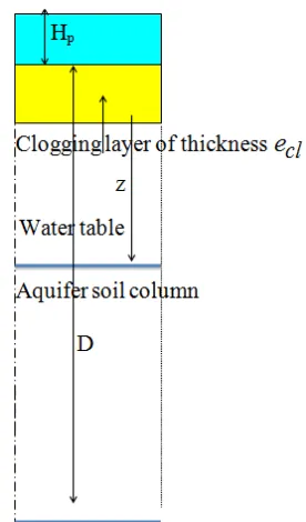
Because the entry pressure of the clogging layer is much higher than that in the aquifer material below, desaturation in the aquifer will occur while the clogging layer remains saturated. Fig. 1 represents schematically the geometry for the one-dimensional case.

Application of Darcy’s law for saturated flow in the clogging layer will give the seepage rate (velocity, dimension of length per time) as:

q

=

K

_cl

(

H

p

+

e

cl

+

h

cI

e

_cl

)

(2) where

K

_cl

is the conductivity of the saturated clogging layer (length per time),

e

_cl

is the thickness of the clogging layer,

H

_p

is the

ponded depth and

h

_cI

is the capillary pressure (head) at the interface between the clogging layer and the aquifer below. In Eq.(1)

H

_p

represents the external pressure force

(expressed as a head),

e

_cl

in the numerator the

force of gravity,

h

_cI

the force of capillarity and

e

_cl

in the denominator the resistance force of viscosity.

Fig. 1. One dimensional aquifer soil column with a clogging layer and a ponded depth

over the riverbed (clogging layer), (Not shown to scale)

If

h

_cI

exceeds the entry pressure in the aquifer,

h

_ce

, then there will be a capillary zone below the clogging layer up to a distance

Z

to the water table, since under desaturation the water table will have receded below the bottom of the clogging layer. Under a steady-state condition

the flow through the clogging layer,

q

_cl

, equals

(4)

The flux

q

is transmitted through the capillary

zone and by Darcy’s law for porous media flow is:

q

*

=

q

K

_a

=

k

rw

(1

+

¶

h

_c

¶

z

)

(3)

where

K

_a

is the conductivity of the aquifer,

k

_rw

is the relative permeability to water,

h

_c

is the capillary pressure and

z

is the vertical coordinate oriented positive downward and with origin at the bottom of the clogging layer. The Brooks-Corey power expressions for capillary pressure and relative permeability in terms of

normalized water content

q

*

=

q

-

q

r

q

_s

-

q

_r

(4) where

q

_s

is the saturated water content and

q

_r

is the residual water content, are:

h

_c

=

h

_ce

(

q

*

)

-

M

(5a)

k

_rw

=

(

q

*

)

p

(5b)

except that when

0 £

h

_c

£

h

_ce

then:

k

_rw

=

1

. The parameter

a

is:

a

=

p

M

(6).

Expressing relative permeability in terms of capillary pressure one obtains:

k

_rw

=

(

h

_c

*

)

-

a

(7)

h

_c

*

=

h

c

h

_ce

(8)

Substitution in Eq.(3) yields:

q

*

=

(h

_c

*

)

-

a

(1

+

h

_ce

¶

h

c

*

¶

z

)

(9)

Solving for

z

from Eq.(3) one obtains:

dz

=

h

_ce

k

rw

dh

c

*

q

*

-

k

_rw

(10)

Integration of Eq.(10) between the interface

(where

h

_c

=

h

_cI

³

h

_ce

) and the water table

(where

h

_c

=

0

) one obtains the depth to the water table:

Z

=

h

_ce

k

rw

dh

c

*

q

*

-

k

_rw

h

_cI*

0 ò

(11)

Breaking the integral into two parts, one for the

range

h

_cI

*

³

h

_c

*

³

1

and the other for the

range

1 ³

h

_c

*

³

0

(where

k

_rw

= 1) one obtains:

Z

=

h

_ce

k

rw

dh

c

*

q

*

-

k

_rw

h

_cI*

1 ò

+

h

_ce

dh

c

*

q

*

-

1

0 ò

(12)

which can be rewritten:

Z

=

h

ce

1 -

q

*

+

1 q

*

du

1 q

*

-

u

a

1 h

_cI

*

ò

(13)

given that in the capillary fringe

k

_rw

=

1

. The first term on the right hand side of Eq. (13) represents the thickness of the capillary fringe under flow conditions. Note that under flowing conditions the thickness of the capillary fringe is not the same as it is under hydrostatic conditions

where it is simply

h

_ce

. Note also that the thickness increases in the case of infiltration but

decreases in the case of evaporation

(

q

*

£

0

). It is shown in Appendix 2 that approximating the capillary fringe thickness by its hydrostatic value has very little impact on the accuracy of the estimate of the incipient desaturation criterion. This is a very practical result.

The second term is the contribution of the unsaturated zone from below the bottom of the clogging layer to the top of the capillary fringe.

(5)

relation of Z with q the flow through the clogging layer at incipient desaturation as:

Z=h_ce 1

1-q*

=h_ce 1

1-Kcl

K_a(

H_p+e_cl+h_ce e_cl )

(14)

That distance, the thickness of the capillary fringe must be positive so that one deduces a constraint on the contrast between the clogging layer conductivity and that of the aquifer below for incipient desaturation to occur since

K

_cl

K

_a

(

H

_p

+

e

_cl

+

h

_ce

e

_cl

)

must be less than 1 for

Z

to be positive:

K

_cl

K

_a

£

e

_cl

H

_p

+

e

_cl

+

h

_ce

(15)

From Eq.(14) one can also derive the value of the ponded depth that will lead to incipient desaturation in association with a given depth to

the water table and a ratio

K

a

K

_cl

:

H_p£e_cl(Ka

K_cl-1)-hce(1+ e_cl

Z K_a K_cl)

(16)

which, with a different notation, is precisely the same as Eq. (9.4.80) [20].

(If the conductivities in the two layers are the same Eq. (16) shows that for desaturation to

occur at the interface a suction (

H

_p

£

0

) must be introduced at the surface of the riverbed, which is to be expected physically).

There is a problem with the one-dimensional approach. In the derivation nothing is said on how this steady-state flux through the clogging layer and the capillary zone above the water table is transmitted through the aquifer below the water table. For that flow to be transmitted a gradient of head must exist in the aquifer. Given Darcy’s law in the aquifer saturated zone then there must exist a constant gradient of capillary pressure so that:

q

_cl

*

=

q

_cz

*

=

q

*

_aq

=

q

*

=

1 +

¶

h

c

¶

z

(17)

which means that at any depth

h

below the water table there must be a capillary pressure of

value

_h

_c

_{= -}

_h

₍₁

_-

_q

*

₎

or equivalently that there

is a water pressure:

_p

w

=

r

w

g

h

(1

-

q

*

)

(18)

where

_r

w

g

is the specific weight of water.

Under hydrostatic condition (with an impervious bottom for the aquifer) the water pressure is

p

_w

=

r

_w

g

h

. What this one-dimensional derivation implies is that there is an invisible hand [25] that maintains a water pressure in the soil column which is neither hydrostatic nor zero and there is a constant water pressure gradient through the column whether very short or extending to the center of the earth. For a given set of parameters it adjusts itself to accommodate the value of the ponded depth, as

it adjusts to the value of

q

*

. It is a little bit like saying that if there is a ponded depth and the bottom of the aquifer was initially impervious, the bottom of the aquifer would become a little less impervious to allow the flux to pass through, and even more pervious to let higher fluxes to pass through. The instructive discussion in Bear’ book was to introduce the reader to the complexity of saturated-unsaturated flow problems in the presence of heterogeneities. Perhaps not emphasized enough in the discussion, the book does differentiate correctly between a capillary fringe and an unsaturated zone. Still the derived formulae are not applicable in practice. The problem in that derivation is that the presentation does not make the reader aware enough that a water table aquifer is not just defined by the fact that at the water table the water pressure is atmospheric but that the aquifer is defined also by its boundaries and the boundary conditions exerted at those boundaries. For that reason the problem is inextricably at least two-dimensional.

3. THE TWO-DIMENSIONAL FORMULA-TION

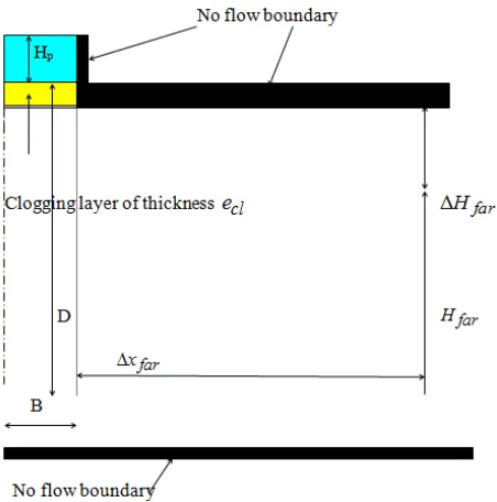
Fig. 2 displays schematically the river cross-section and location of a clogging layer (riverbed) for a non-penetrating river.

(6)

Fig. 2. Non-penetrating river cross-section and location of clogging layer

Fig. 3. Flow and potential lines, ratio

K

cl

K

_a

=

0.1

of potential and streamlines for a non-penetrating river for a ratio K_cl

K_a =0.1

. The results were

obtained [15] using a groundwater model for saturated flow [8].

Selected values for Fig. 3 were the following: B = 20 meters, D=100 meters, _e_cl₌_0.5 meters,

h_ce=0.2 meters, H_p=0.

4. ANALYTICAL DETERMINATION OF

THE LATERAL SEEPAGE FLOW

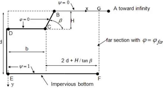
Fig. 4 displays the geometry of the problem for a trapezoidal cross-section.

In Fig. 4, b is the half width of river and d is the aquifer thickness. Studies [12,14,15] have shown that under conditions of saturated flow the

discharge on one side of the cross-section, under assumption of symmetry of heads on the sides of the river, can be expressed in the form:

Q

=

K

_a

L

G

(H

_S

-

H

_far

)

(19)

where L is the longitudinal length of the river reach,

H

_S

is the head in the river and

H

_far

is

the head at a far “enough” distance (conservatively estimated to be twice the aquifer thickness [26]) so that by that distance the flow is essentially horizontal and

G

is the one-sided (Stream-Aquifer Flow Exchange, SAFE) dimensionless conductance [12,14].

(7)

Fig. 4. Cross-section geometry and corner points nomenclature (Not drawn to scale)

the river, line BCD in Fig. 4, on one hand and on the other hand, the vertical line across the aquifer located at the far distance from the bank of the river, vertical line GF in Fig. 4.

It is derived mathematically as the stream function difference,

_D

_y

, between the center of the cross-section and the top of the side of the cross-section, divided by the potential difference,

D

j

, on the perimeter of the cross-section where

j

=

0

and that at the far distance vertical boundary,

_j

far, so that

G = D

y

/

D

j

. One

selects for

_D

_y

arbitrarily the value 1 and one determines analytically the value of the potential

j

_far at the far distance.

G

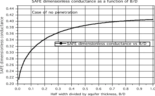
is thus evaluated exactly [12,14] and is a function of the wetted perimeter of the river cross-section.

For example the formula for the case of a non-penetrating river is:

G_flat= 1

2 1+1

pln

2

1-e-p

B D

é

ë ê ê ê

ù

û ú ú ú ì

í ï

î ï

ü ý ï

þ ï

(20)

where

B

is the half width of the river cross-section and D is the thickness of the aquifer.

5. DERIVATION OF CRITERION FOR INCIPIENT DESATURATION

Such derivation has already been presented [27] and is summarized below. The seepage discharge, Q, (volume per unit time) through the

clogging layer, which is saturated, at incipient desaturation, is given by the Darcy velocity, q, (length per time) multiplied by the area through which flow takes place,

BL

:

_Q

₌

_qBL

₌

_{

_K

_cl

₍

H

p

+

e

cl

+

h

ce

e

_cl

)}

BL

(21)

where

H

_p

is the ponded depth. The same

discharge flows from the bottom of the clogging layer to the far distance vertical boundary and has the expression, by application of Eq.(19):

Q=K_aLG(D-e_cl-Z-H_far)=K_aLGDH_far (22)

where

H

_far

is the elevation of the water table

with datum at the bottom of the aquifer at a distance equal to twice the aquifer thickness from the river bank. D is the distance between the top of the clogging layer and the impervious bottom of the aquifer,

G

is the Stream-Aquifer Flow Exchange (SAFE) dimensionless conductance [14,15] and

_D

_H

_faris the difference between the head of the water table below the riverbed,

D

-

e

_cl

-

Z

, and the head at the far distance,

H_far. Equating the right hand sides of Eqs. (21)

and (22) provides the value of q*(and thus

K

_cl

/

K

_a

) at initial desaturation for a given value of the head, _H

far, at the far distance and

values of the other parameters. That value is solution of equation:

DHfar={D-ecl- hce

1-q*

-Hfar}=B

Gq

(8)

6. USE OF THE FORMULAE FOR PRACTICAL APPLICATIONS

questions. First, Given the values of the ratio

K_cl/K_a, of the clogging layer thickness, the ponded depth and the entry pressure, the value of _D_H

far to lead to incipient desaturation can be

deduced as follows:

q

*

=

K

cl

K

_a

(

H

_p

+

e

_cl

+

h

_ce

)

e

_cl

(24)

Then

DH_far=(B

G)q

*₌₍B

G)(

K_cl K_a)

(H_p+e_cl+h_ce) e_cl

(25a)

and more practically:

H_far=(D-e_cl- hce

1-q*

)-B

Gq

* (25b)

Also given a value of _D_H

far for what value of

K_cl/K_awould incipient desaturation occur? For that more complicated question one needs to

solve the second order Eq. (23) for

q

*

and thus

K_cl/K_a.

Defining for simplicity the term:

G

B(D-ecl-Hfar)=u

(26)

the solution for

q

*

is:

q

*

=

(1

+

u

)

-

(1

-

u

)

2

+

4 G

B

h

ce

2

(27a)

or more explicitly:

q

*

=

(1

+

G

B

(

D

-

e

cl

-

H

far

))

-

[1

-G

B

(

D

-

e

cl

-

H

far

)]

2

₊

₄

G

B

h

ce

2

(27b) which leads

to the condition for incipient desaturation:

K

_cl

K

_a

=

q

*

[

e

cl

(

H

_p

+

e

_cl

+

h

_ce

)

]

=

G

B

[

e

_cl

(

H

_p

+

e

_cl

+

h

_ce

)

]

D

H

far

(28)

where

D

H

_far

is the change (drop) in head between the water table below the clogging layer and the water table at the far distance. Once the head drop increases above the value given by Eq.

(28) desaturation occurs.

(9)

For a given value of desaturation will

not occur unless:

K

_cl

K

_a

£

G

B

[

e

_cl

(

H

_p

+

e

_cl

+

h

_ce

)

]

D

H

far

(29)

7. COMPARISON WITH THE

ONE-DIMENSIONAL RESULTS

It is instructive to compare the two-dimensional Eq. (29) with the one-dimensional Eq. (15). As is quite apparent in Eq. (15) the geometric characteristics such as the width of the river and the thickness of the aquifer that is a parameter in the formula for

G

(e.g. see Eq. 20), do not appear. In addition in the one-dimensional analysis the ponded depth in the river appears but per se; no head difference is defined between the river and some point in the aquifer below or laterally at some distance away. In Eq.(29) both _D_H

far and Hp appear and their

physical significance is different. Both influence, in their separate way, the incipient desaturation.

(Eq. 29 may appear singular as

B

tends to zero but

G

also tends to zero as can be seen from the expression in Eq. 20).

Without displaying any figure, showing how the incipient desaturation (i.d.) value of the ratio

K

_cl

/

K

_a

varies with the various parameters, it is clear that for a given set of parameters that ratio varies proportionately to _D_H

far, it varies

inversely proportional to

_H

p , etc. The only

relation that is not obvious is the function of

B

since

G

is also a function of

B

or rather of

B

/

D

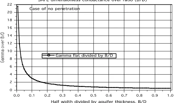
. It is convenient to rewrite Eq. (29) as:

K_cl K_a £{

G

B/D}[

e_cl

(H_p+e_cl+h_ce)](

DH_far D )

(30)

Fig. 5 shows the i.d. ratio

K

cl

K

_a

as a function of

(

B

D

)

for a fixed set of parameters such that

[

e

cl

(

H

_p

+

e

_cl

+

h

_ce

)

]

D

H

_far

D

= 1.

Quite obviously what is plotted is simply: _{ G

B/D}

For a half width B = 10 meters, an aquifer thickness of D = 100 meters, then B/D=0.1. The value of

G

/ (

B

/

D

)

=

3.0527

. For

e

_cl

=

0.5

meters,

_h

_ce

₌

_0.4

meters,

_H

p

=

0.8

meters and

D

H

_far

=

2

meters, then the value of the ratio

K_cl/K_afor incipient desaturation would have to be:

K_cl

K_a =3.0527[

0.5 (0.8+0.5+0.4)](

2.0

100)=0.018

Fig. 6 shows the variation of

G

as a function of B/D.

(10)

8. DISCUSSION

The two-dimensional analysis presented here is limited to the case of an impervious boundary at the bottom of the aquifer. Other boundary conditions could be investigated such as those referred to by Rushton [11] as Conditions, A, and A’. In this work only condition B was considered directly, that is the case when the bottom of the water table aquifer is an impervious boundary. Condition A’ can be solved analytically quite easily but it would be a situation very rarely encountered in practice. Nevertheless the availability of analytical formulae for these different conditions would be desirable.

The determination of the trigger for incipient desaturation is useful but further work needs to be done to determine the flow exchange after desaturation has taken place. Finally one needs to secure a description of what happens to the flow exchange under transient conditions. What is presented here is just a building block toward fairly simple, approximate yet accurate, analytical solutions for the more complex problems. These have already been the subject of other articles [16,17, 27,28].

9. CONCLUSION

An analytical solution is presented for the condition of incipient desaturation to occur between a river and an aquifer that were initially in saturated connection. The criterion for the initiation of incipient desaturation is fully algebraic and exact. Simple formulae display the factors that influence the phenomenon be they the conductivities of the clogging layer or of the aquifer below, the geometric characteristics of the river such as its width and depth, the aquifer thickness, the ponded depth and the head difference between the river and the far distance away from the bank of the river. The derivation would not have been possible without the previous analytical derivations of the SAFE dimensionless conductance,

G

, for various cross-section geometries.

The derivations show that the thickness of the capillary fringe is not a constant but depends upon the exchange flow rate. Fortunately it is shown that for practical situations neglecting the change in thickness of the capillary fringe due to flow, as opposed to its hydrostatic value, has essentially no impact on the accuracy of the criteria for incipient desaturation. Even when there is a drop of head at the far distance

amounting to about 10% of the aquifer thickness the error of overestimation is less than 2%. Thus neglecting the change of thickness of the capillary fringe due to flow as opposed to its value under hydrostatic conditions has very limited effect on the accuracy of estimates, including the seepage rate.

ACKNOWLEDGEMENTS

Morel-Seytoux is Emeritus Professor of Civil and Environmental Engineering at Colorado State University. Morel-Seytoux’ research for this paper was conducted while a visiting scholar at Stanford University in the department of Civil and Environmental Engineering. Data used to generate the results and the figures can be obtained from Morel-Seytoux at Hydroprose International Consulting.

COMPETING INTERESTS

Author has declared that no competing interests exist.

REFERENCES

1. Bredehoeft JD, Kendy E. Strategies for offsetting seasonal impacts of pumping on a nearby stream. Groundwater. Tallahassee, Florida. 1990;46(1):23-29. 2. Dogrul EC. Integrated water flow model

(IWFM v4.0): Theoretical documentation. Sacramento, (CA): Integrated Hydrological Models Development Unit, Modeling Support Branch, Bay Delta Office, California Department of Water Resources; 2012.

3. Foglia L, McNally A, Harter TJ. Coupling a spatiotemporally distributed soil water budget with stream-depletion functions to inform stakeholder-driven management of groundwater dependent ecosystems. Water Resour. Res. 2013;49: 7292–7310.

4. Harbaugh AW. MODFLOW-2005 - The U.S. Geological Survey modular ground-water model-The ground-water flow process. U.S. Geological Survey Techniques and Methods 6-A16. 2005;253.

(11)

Environmental Modeling Forum, Sacramento; 2013.

Available: http://www.cwemf.org

6. McDonald M, Harbaugh A. A modular three-dimensional finite-difference ground-water flow model: Techniques of Water-Resources Investigations of the United States Geological Survey, Book 6, Chapter A1. 1988;586.

7. Kumar M, Bhatt G, Duffy CJ. PIFM. An efficient domain decomposition framework for accurate representation of geodata in distributed hydrologic models. International Journal of Geographical Information Science. 2009;23(12):1569–1596.

8. Kinzelbach W, Rausch R. Grundwassermodellierung. Gebrüder Borntraeger Verlag,Berlin.1995;283. 9. MIKE_SHE_Printed_V1.pdf. User Manual.

User Guide. Particularly sections 7.6.2 to 7.6.6. 2013;202-212.

DOI:

ORG/10.9734/IJECC/2019/V9I330106 10. Therrien R, McLaren RG, Sucdicky EA,

Park YJ. HydroGeoSphere. A three-dimensional numerical model describing fully integrated subsurface and surface flow and solute transport. Université Laval and University of Waterloo. 2012;166. 11. Rushton K. Representation in regional

models of saturated river-aquifer interaction for gaining/losing rivers. J. Hydrol. 2007;334:262-281.

12. Morel-Seytoux HJ. The turning factor in the estimation of stream-aquifer seepage. Groundwater. 2009;47(2):205-212.

13. Mehl S, Hill MC. Grid-size dependence of Cauchy boundary conditions used to simulate stream-aquifer interaction. Adv. Water Resour. 2010;33:430-442.

14. Morel-Seytoux HJ, Steffen Mehl, Kyle Morgado. Factors influencing the stream-aquifer flow exchange coefficient, Groundwater; 2013.

DOI: 10.1111/gwat.12112, 7

15. Miracapillo C, Morel-Seytoux HJ. Analytical solutions for stream-aquifer flow exchange under varying head asymmetry and river penetration: Comparison to numerical solutions and use in regional groundwater models, Water Resour. Res. 2014;50. DOI:10.1002/2014WR015456

16. Morel-Seytoux HJ. MODFLOW’s River Package: Part 1: A Critique. Physical Science International Journal. PSIJ. 2019a;22(2):1-9.

Article no.PSIJ.49757

DOI: 10.9734/PSIJ/2019/v22i230129 17. Morel-Seytoux HJ. MODFLOW’s river

package: Part 2: Correction, combining analytical and numerical approaches. Physical Science International Journal. 2019b;22(3):1-23.

Article no.PSIJ.49758

DOI: 10.9734/PSIJ/2019/v22i330131 18. Osman YZ, Michael P. Bruen. Modelling

stream–aquifer seepage in an alluvial aquifer: An improved loosing-stream package for MODFLOW. Journal of Hydrology. 2002;264:69–86.

19. Fox, G. A., 2003. Improving MODFLOW’s RIVER Package for unsaturated stream/aquifer flow. Proc. Hydrology Days 2003, 56-67l

20. Bear J. Dynamics of Fluids in Porous Media. American Elsevier, New York, N.Y. 1972;764.

21. Fox GA, Gordji L. Consideration for unsaturated flow beneath a streambed during alluvial well Depletion; 2007.

DOI:10.1061/_ASCE_1084-0699_2007_12:2_139.

22. Fox GA, Durnford DS. Unsaturated hyporheic zone flow in stream/aquifer conjunctive systems. Adv. Water Resour. 2003;26(9):989–1000.

23. Morel-Seytoux HJ. Introduction to flow of immiscible liquids in porous media. Chapter XI in Flow through Porous Media. R. deWiest, Editor, Academic Press. 1969;455-516.

24. Corey AT. Mechanics of heterogeneous fluids in porous media. Water Resources Publications. Fort Collins, Colorado. 1977; 259.

25. Smith A. The Wealth of Nations. W. Strahon and T. Cadell, London; 1776. 26. Haitjema H. Comparing a

three-dimensional and a dupuit-forcheimer solution for a circular recharge area in a confined aquifer. J. Hydrol. 1987;91:83-101.

27. Morel-Seytoux HJ. Analytical solutions using integral formulations and their coupling with numerical approaches. Groundwater. 2014;9.

DOI:10.1111/gwat.12263

(12)

APPENDIX 1. NOTATION

B

or

b

: Half width of the cross-section bottom

d

_p: Degree of penetration, H

D

or

d

: Aquifer thickness

DH

_far (or

D

H

_far

): Drop of head between the top of the water table mound and the far distance

e

_cl

: Thickness of clogging layer (length)

e

_cl

*

: ratio

e

cl

h

_ce

h

: Generally a height or head with dimension of length

h

_a

: Head in the aquifer at some distance from the river bank

h

_c

: Capillary pressure or capillary pressure head (dimension of length)

h

_ce

: Drainage entry pressure (length)

h

_cI

: capillary pressure at the interface (bottom of the clogging layer)

h

_cI

*

: ratio

h

cI

h

_ce

H

: Penetration depth of river into the aquifer

H

_far

: Head at the far distance

H

_p

: Ponded depth above the riverbed (clogging layer)

H

*

_p

: Ratio

H

p

h

_ce

H

_S

: Head in the river

k

_rw

: Relative permeability

k

_rwI

: Relative permeability at interface on the aquifer side

K

: Generally a saturated hydraulic conductivity (dimension of velocity)

K

_a

: Aquifer hydraulic conductivity

K

_cl

: Clogging layer hydraulic conductivity

L

: Length of river reach

M

: Exponent in the power (Brooks-Corey) expression for capillary pressure as a function of normalized water content

p

: Exponent in the power expression for relative permeability as a function of normalized water content

q

: Seepage velocity (flow rate) in the Darcy sense

q

_aq

: Flow rate through the aquifer below the water table

(13)

q

_cz

: Flow rate through the capillary zone above the water table

q

*

: Normalized seepage velocity,

q

K

_a

q

_id

*

: Normalized seepage rate occurring at incipient desaturation

Q

: Total seepage discharge (volume per time)

x

_far

: Distance from the center of the river cross-section to the far distance

z

: Vertical coordinate oriented positive downward with origin at the bottom of the clogging layer

Z

: Depth from the bottom of the clogging layer to the water table mound,

Z

*

: Normalized value of

Z

,

Z

h

_ce

a

: Ratio

p

M

q

: Generally water content (dimensionless)

q

_S

: Saturated water content

q

_r

: Residual water content

q

*

: Normalized water content, =

q

-

q

res

q

_S

-

q

_res

h

: Arbitrary depth below the water table

G

: One sided SAFE (Stream Aquifer Flow Exchange) dimensionless conductance

G

_flat

:

G

In case of no penetration of the river or for a flat recharge zone

D

H

_far

(or

DH

_far

) : drop of head between the top of the water table mound and the far distance

D

x

_far

: Distance from river bank to far distance

j

=

0

: Potential on the wetted perimeter of the river cross-section

j

_far

: Potential at the vertical far distance from the river bank

y

: Stream function of value 1 at center of cross-section and of value 0 at the upper most wetted point on the river bank

(

¶

h

c

¶

z

)

I

: Capillary gradient at the interface on the aquifer side

APPENDIX 2. Neglecting the influence of flow rate on size of capillary fringe

(14)

DH_far={D-e_cl- hce

1-q*

-H_far} (1) as

{

D

-

e

cl

-

h

ce

-

H

far

}

(2) naturally only valid if

q

*

much

<

1

.

The error on

_K

_cl

_/

_K

_a will be directly proportional to the overpredicting factor:

{

D

-

e

_cl

-

h

_ce

-

H

_far

} / {

D

-

e

_cl

-

h

ce

1 -

q

*

-

H

_far

}

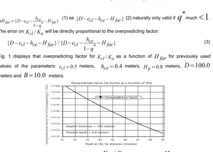
(3)

Fig. 1 displays that overpredicting factor for K_cl/K_a as a function of

_H

_far

for previously used

values of the parameters:

_e

_cl

₌

_0.5

meters,

h

_ce

=

0.4

meters,

_H

_p

₌

_0.8

meters,

D

=

100.0

meters and

B

=

10.0

meters.

Fig. 1. Overprediction factor for

K

_cl

/

K

_a

as a function of

H

_far

One can see that even when there is a drop of head at the far distance amounting to about 10% of the aquifer thickness the error of overestimation is less than 2%.

Fig. 2. shows a similar pattern for different parameters.

Fig. 2. Overprediction factor for