Simplified spiking neural network architecture and STDP learning algorithm applied to image classification

(1)

R E S E A R C H

Open Access

Simplified spiking neural network architecture

and STDP learning algorithm applied to image

classification

Taras Iakymchuk

*

, Alfredo Rosado-Muñoz, Juan F Guerrero-Martínez, Manuel Bataller-Mompeán

and Jose V Francés-Víllora

Abstract

Spiking neural networks (SNN) have gained popularity in embedded applications such as robotics and computer vision. The main advantages of SNN are the temporal plasticity, ease of use in neural interface circuits and reduced computation complexity. SNN have been successfully used for image classification. They provide a model for the mammalian visual cortex, image segmentation and pattern recognition. Different spiking neuron mathematical models exist, but their computational complexity makes them ill-suited for hardware implementation. In this paper, a novel, simplified and computationally efficient model of spike response model (SRM) neuron with spike-time dependent plasticity (STDP) learning is presented. Frequency spike coding based on receptive fields is used for data representation; images are encoded by the network and processed in a similar manner as the primary layers in visual cortex. The network output can be used as a primary feature extractor for further refined recognition or as a simple object classifier. Results show that the model can successfully learn and classify black and white images with added noise or partially obscured samples with up to×20 computing speed-up at an equivalent classification ratio when compared to classic SRM neuron membrane models. The proposed solution combines spike encoding, network topology, neuron membrane model and STDP learning.

Keywords: Spiking neural networks - SNN; STDP; Visual receptive fields; Spike coding; Embedded system; Artificial neuron; Image classification

1 Introduction

In the last years, the popularity of spiking neural net-works (SNN) and spiking models has increased. SNN are suitable for a wide range of applications such as pattern recognition and clustering, among others.There are exam-ples of intelligent systems, converting data directly from sensors [1,2], controlling manipulators [3] and robots [4], doing recognition or detection tasks [5,6], tactile sensing [7] or processing neuromedical data [8]. Different neu-ron models exist [9] but their computational complexity and memory requirements are high, limiting their use in robotics, embedded systems and real-time or mobile applications in general.

*Correspondence: [email protected]

GPDS, ETSE, University of Valencia, Av. Universitad, 46100 Burjassot, Valencia, Spain

Existing simplified bio-inspired neural models [10,11] are focused on spike train generation and real neuron modeling. These models are rarely applied in practical tasks. Some of the neuronal models are applied only for linearly separable classes [12] and focus on small network simulation.

Concerning hardware implementation, dedicated ASIC solutions exist such as SpiNNaker [13], BrainScaleS [14], SyNAPSE [15] or others [16], but they are targeted for large-scale simulations rather than portable, low-power and real-time embedded applications. The model we propose is mainly oriented for applications requiring low-power, small and efficient hardware systems. It can also be used for computer simulations with up to ×20 speed-up compared to classic SRM neuron membrane model. Nowadays, due to a continuous decrease in price and increase in computation capabilities, combined with

(2)

the progress in high-level hardware description language (HDL) synthesis tools, configurable devices such as FPGA can be used as efficient hardware accelerators for neu-romorphic systems. A proposal was made by Schrauwen and Van Campenhout [17] using serial arithmetic to reduce hardware resource consumption, but no train-ing or weight adaptation was possible. Other solution, presented by Rice et al. [18] used full-scale Izhikevich neu-rons with very high resource consumption (25 neuneu-rons occupy 79% of logic resources in a Virtex4 FPGA device), without on-line training.

Computation methods used for FPGA dramatically dif-fer from classic methods used in Von Neumann PCs or even SIMD processing units like GPUs or DSPs. Thus, the required SNN hardware architecture must be differ-ent for reconfigurable devices, opening new possibilities for computation optimization. FPGA are optimal for mas-sive parallel and relatively simple processing units rather than large universal computational blocks as is in case of SNN, including lots of multiply-add arithmetic blocks and vast quantities of distributed block RAM [19]. This work describes computation algorithms properly modeling the SNN and its training algorithm, specifically targeted to benefit from reconfigurable hardware blocks. The pro-posed solution combines spike encoding, topology, neu-ron membrane model and spike-time dependent plasticity (STDP) learning.

2 Spiking neural networks model

Spiking neural networks are considered to be the third generation of artificial neural networks (ANN). While classic ANN operate with real or integer-valued inputs, SNN process data in form of series of spikes called spike trains, which, in terms of computation means that a single bit line toggling between logical levels ‘0’ and ‘1’ is required. SNN are able to process temporal pat-terns, not only spatial, and SNN are more computation-ally powerful than ANN [20]. Classic machine learning methods perform poorly for spike coded data, being unsuitable for SNN. As a consequence, different training and network topology optimization algorithms must be used [9,21].

The SNN model used in this work is the feed-forward network, each neuron is connected to all the neu-rons in the next layer by a weighted connection, which means that the output signal of a neuron has a differ-ent weighted potdiffer-ential contribution [22]. Input neurons require spike trains and input signals (stimuli) need to be encoded into spikes (typically, spike trains) to further feed the SNN.

An approximation to the functionality of a neuron is given by electrical models which reproduce the function-ality of neuronal cells. One of the most common mod-els is the spike response model (SRM) due to the close

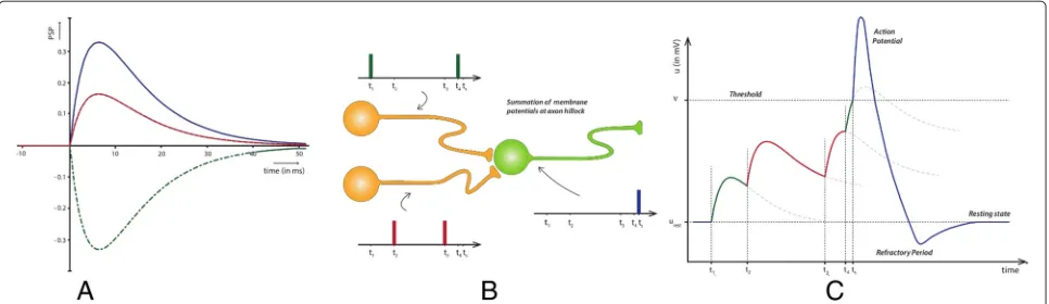
approximation to a real biological neuron [23,24]; the SRM is a generalization of the ‘integrate and fire’ model [9]. The main characteristic of a spiking neuron is the membrane potential, the transmission of a single spike from one neuron to another is mediated by synapses at the point where neurons interact. In neuroscience, a trans-mitting neuron is defined as a presynaptic neuron and a receiving neuron as a postsynaptic neuron. With no activity, neurons have a small negative electrical charge of−70 mV, which is called resting potential; when a sin-gle spike arrives into a postsynaptic neuron, it generates a post synaptic potential (PSP) which is excitatory when the membrane potential is increasing and inhibitory when decreasing. The membrane potential at an instant is cal-culated as the sum of all present PSP at the neuron inputs. When the membrane potential is above a critical thresh-old value, a postsynaptic spike is generated, entering the neuron into a refractory period when the membrane remains overpolarized, preventing neurons from generat-ing new spikes temporarily. After a refractory period, the neuron potential returns to its resting value and is ready to fire a new spike if membrane potential is above the threshold.

The PSP function is given by Equation 1, where τm andτsare time constants to control the steepness of rise and decay, and t is the time after the presynaptic spike arrived.

PSP(t)=e(τ−mt)−e

−t

τs

, (1)

Figure 1A shows different PSP as a function of time (ms) and weight value, being excitatory in case of red and blue lines, and inhibitory in case of a green line.

Let us consider the example shown in Figure 1B where spikes from two presynaptic neurons trigger an excitation PSP in a postsynaptic neuron. The spike train generated by the presynaptic neurons will change the membrane potential calculated as the sum of individual PSPs gen-erated by incoming spikes. When membrane potential reaches the threshold, the neuron fires a spike at the instant ts. Graphically it is shown on Figure 1C. If we denote the threshold value as υ, the refractory periodη is defined according to Equation 2 [24]. This equation describes a simple exponential decay of membrane charge, being H(t) the Heavyside step function, H(t) = 0, for t<0 andH(t)=1 fort>0;τris a constant defining the steepness of the decay.

η(t)= −υe

t

τr

H(t) (2)

(3)

Figure 1Postsynaptic potential function (PSP) with weight dependency.(A)Red line is for_ω₌1, green for_ω_{= −}1 and blue is for_ω₌0.5.

(B)Two neurons (yellow) generate spikes, which are presynaptic for next layer neuron (green).(C)Membrane potential graph for green neuron. Presynaptic spikes raise the potential; when the potential is above threshold, a postsynaptic spike is generated and the neuron becomes overpolarized.

neuronjat timetand the time difference between these two events is t− t_i(g). The travelling time between two neurons for a spike is defined by Equation 3 wheredji is the delay of synapse value.

tji=t−ti(g)−dji (3) When a sequence of spikesFi =

t_i(g),. . .,tK_i

arrives to a neuronj, the membrane potential changes accord-ing to the PSP function and refractory period, and thus, an output spike train is propagated by neuronjasFj =

t(_jf),. . .,t_jN. The equation for thej-th neuron potential

Pjis obtained according to Equation 4, where the refrac-tory period is also considered.

Pj(t)= K

i

t(_ig)∈Fi

wijPSP(tji)+

t(jf)∈Fj

ηt−t_j(f) (4)

These equations define the SRM, which can be mod-eled by analog circuits since the PSP function can be seen as a charging and discharging RC circuit. How-ever, this model is computationally complex when used in digital systems. We propose to use a simplified model

(4)

Figure 3STDP curve used for learning.This type of curve has stronger depression value than potentiation, increasing specificity.A+=0.6,A−= 0.3,τ+=8,τ−=5.

with linear membrane potential degradation with similar performance and learning capabilities as the classic SRM.

3 Simplified spiking neural model

The classic leaky integrate-and-fire (LIF) model [9] and its generalized form (SRM) are widely used as a neuron model. However, LIF spiking neuron models are compu-tationally complex since non-linear equations are used to model the membrane potential. However, simplification might be defined in order to reduce computational com-plexity by proposing a simplified membrane model. Let us describe the membrane potentialPtas a function of time and incoming spikes. Time units are counted in discrete time form as the model is intended to be used in digital circuits. For ann-input SNN, during the non-refractory period, each incoming spike Sit,i =[1..n] increases the membrane potentialPt by a value of synapse weightWi. In addition, the membrane potential is decreasing by a constant valueD, every time instant. This process can be described by Equation 5, which corresponds to a simpli-fied version of Equation 4 in a LIF model.

Pt=

⎧ ⎪ ⎪ ⎨ ⎪ ⎪ ⎩

Pt−1+ n

i=1

WiSit−D, if Pmin<Pt−1<Pthreshold Prefract, if Pt−1≥Pthreshold

Rp, if Pt−1≤Pmin

(5)

Thus, instead of an initial postsynaptic potential ramp in the spike response model, the instant change of mem-brane potential allows a neuron to fire immediately in the next clock cycle after the spike arrives.

At each time instantt, if membrane potentialPtis big-ger than the resting potential Rp = 0, it degrades by a fixed valuePt=Pt−1−D. The resulting PSP function will be a saw-like linear function, which is easily implemented by a register and a counter, contrary to classic non-linear PSP models based on look-up tables or RAM/ROM for non-linear equations. The value of constant D is cho-sen relevant to the maximum presynaptic spike rate and the number of inputs. An example of membrane poten-tial dynamics is shown in Figure 2. WhenPt >Pthreshold, the neuron fires a spike, the membrane potential becomes Pt = Prefract (resting potential) and a refractory period

(5)

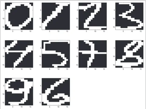
Figure 5Patterns for network training of 10 hand written digits (Semeion dataset).

counter starts. Instead of a slow repolarization of mem-brane after the spike, the neuron is blocking its inputs for timeTrefract, and holds membrane potential atPrefractlevel during this time. To avoid strong negative polarization of membrane, its potential is limited by Pmin. Despite the model of the neuron is linear, the network can produce non-linear response by tuning the weights of previous layer inputs.

3.1 Spike-time dependent plasticity learning

STDP is a phenomenon discovered in live neurons by Bi and Poo [25] and adapted for learning event-based networks. STDP learning is an unsupervised learning algorithm based on dependencies between presynap-tic and postsynappresynap-tic spikes. In a given synapse, when a postsynaptic spike occurs in a specific time window after a presynaptic spike, the weight of this synapse

(6)

Figure 7Three receptive fields on the 10×10 input space.Blue field corresponds to the neuron(A)(3,3 in input matrix). Green field corresponds to neuron(B)(6,5) and orange corresponds to neuron

(C)(10,10). Note that only active part or RF is shown.

is increased. If the postsynaptic spike appears before the presynaptic spike, a decrease in the weight occurs assuming that inverse dependency exists between pre-and postsynaptic spikes. The strength of the weight change is a function of time between presynaptic and

postsynaptic spike events. The used function is shown on Figure 3.

For STDP learning, The classic asymmetric reinforce-ment curve is used, taking time units (TUs) as argureinforce-ment. The learning function is described in Equation 6 where A−andA+are constants for negative and positive values of time difference t between presynaptic and postsy-naptic spikes, determining the maximum excitation and inhibition values;τ−,τ+are constants characterizing the steepness of the function.

STDP(t)=w=

⎧ ⎨ ⎩

A−exp∗_τ−t, if t≤ −2 0, if −2< t<2 A+exp∗_τ+t, if t≥2

(6)

The learning rule (weight change) is described by Equation 7. The weights are always limited by wmax ≥ w≥wmin. The desired distance between presynaptic and postsynaptic spike is unity and the STDP window is [2..20] TUs in both directions. The weight change rateσcontrols the weight adaptation speed.

wnew=

wold+σw(wmax−wold), if w>0

wold+σw(wold−wmin), if w≤0 (7) Since unsupervised learning requires competition, lat-eral inhibition was introduced and thus, the weights of

(7)

the winner neurons (first spiking neurons) are increased while other neurons suffer a small weight reduction value. Tests showed that depressing the weights of the non firing neurons decrease the amount of noise in the net-work. The depression of synapses that do not fire at all was added in order to eliminate ‘mute’ synapses (inac-tive synapses), reducing the network size and improving robustness against noise. This training causes a side effect since, for weight increase, spike-intense patterns require a higher membrane threshold, avoiding the patterns with low spike intensity to be recognized by the network. This is solved by introducing negative weights, preventing neu-rons from reacting on every pattern and increasing the specificity of classifier.

4 Visual receptive fields

The visual cortex is one of the best studied parts of the brain. The receptive field (RF) of a visual neuron is an

area of the image affecting the neural input. The size and shape of receptive fields vary depending on the neu-ron position and neuneu-ron task. A variety of tasks can be done with RFs: edge detection, sharpening, blurring, line decomposition, etc. In each subsequent layer of the visual cortex, receptive fields of the neurons cover bigger and bigger regions, convolving the outputs of the previous layer.

Mammalian retinal ganglion cells located at the cen-ter of vision, in the fovea, have the smallest receptive fields, and those located in the visual periphery have the largest receptive fields [26]. The large receptive field size of neurons in the visual periphery explains the poor spatial resolution of human vision outside the point of fixation, together with photoreceptor density and optical aberra-tions. Only a few cortical receptive fields resemble the structure of thalamic receptive fields, some fields have elongated subregions responding to dark or light spots,

(8)

while others do not respond to spots at all. In addition, the implementation of a receptive field is a first stage of sparse coding [27] where the neurons are reacting to shapes, not single pixels. The receptive field model proposed here shows a good approximation to the real behavior of primary visual cortex.

4.1 Receptive field neuron response

The neurons in the receptive or sensory layer generate a responseRRF defined by Equation 8, as the calculation of Frobenious inner product of the input imageS with the receptive fieldFof the neuron and calculation of the sum of input stimuli. This operation is similar to normal 2D convolution, the only difference that in convolution kernel is rotated by 180◦.

RRF = I

i J

j

SijFij (8)

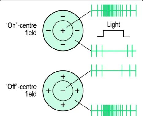
The matrixF defines a receptive field (RF) of the neu-ron, beingIthe X axis andJthe Y axis sizes of input image S. While the shape and size of receptive field can be arbi-trary, in the mammalian visual cortex, there are several distinct types of receptive fields. Two common types are off-centered and on-centered as shown in Figure 4. These RFs can be used as line detectors, small circle detectors or perform basic feature extraction for higher layers. Sim-ple classification tasks such as the inclination of a line, circle or non-circle object and others can be performed by this type of single-layer receptive field neurons. Once input and weights are normalized, the maximum excita-tion of a certain output neuron will be achieved when the input exactly matches the weight matrix, providing pattern classification when weights are properly adjusted. Sensory layer neurons generate spikes at a frequency proportional to their excitation. As the frequency of a fir-ing neuron cannot be infinite, the maximum firfir-ing rate is limited, and thus, the membrane potential is normalized.

(9)

The spiking response firing rate (FRn) is described by Equation 9, whereRPmax is the defined minimum refrac-tory period and max(R)is the maximum possible value of membrane potential.

FRn=

₁

RPmax∗_maxRRF₍_R₎, if RRF>0

0, if RRF≤0

(9)

5 Software simulation and results

A subset of Semeion handwritten digit dataset [28] was used to test the new algorithms and proof the validity of simplifications. Matlab software was used. The dataset consists on 1,593 samples of black and white images of handwritten digits 0 to 9 (160 samples per digit), 16×16 pixels size as shown in Figure 5. The training set consisted of 20 samples for each class (each digit) with 5% of uniform random noise added to every sample fed into the SNN.

5.1 Image encoding

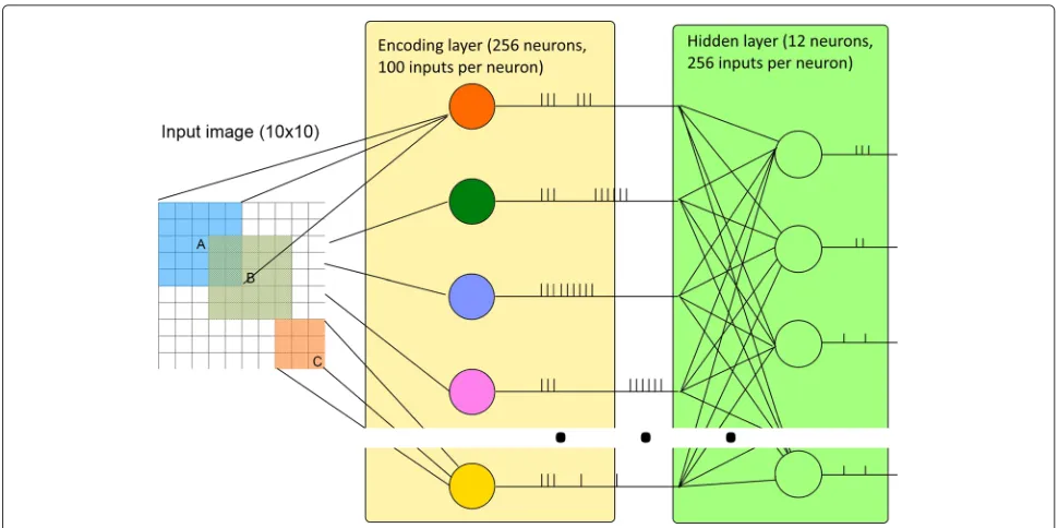
In the described experiment, a 5×5 on-centered recep-tive field was used. This receprecep-tive field was weighted in a [−0.5,..,1] range according to Manhattan distance to the center of the field. A 16×16 pixel input is processed by a 16×16 encoding neuron layer (256 neurons), obtain-ing a potential value for each input which will be further converted into spikes. The coding process using the 5× 5 receptive field is shown in Figure 6A,B. The neural response, shown in Figure 6C is the membrane potential map, further converted into spike trains whose spiking frequency is proportional to such potential, as shown in Figure 6D. The same procedure is repeated for all input neurons. The receptive fields of the neurons are

over-Figure 11Neurons weights representation after STDP training. Ten out of sixteen neurons learnt to discriminate all ten numbers in the SEMEION dataset.

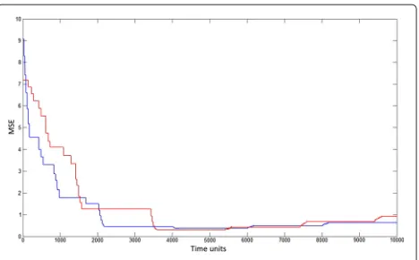
Figure 12MSE for single pattern during learning.Red line represents simplified model, and blue represents classic SRM. It can be seen that, after 5,000 TU, neuron becomes overtrained for both models.

lapping; an example of three receptive fields is shown in Figure 7 where, in case C, a part of the RF lay outside the input space, and thus, that part is not contributing to membrane potential.

5.2 Network architecture

The proposed SNN consists of 2 layers, an encoding layer of 256 neurons with an on-centered 5×5 pixel RF and second layer of 16 neurons using the simplified SRM. Experimental testing showed that, for proper competitive-ness in the network, the number of neurons should be at least 20% greater than the number of classes and thus, 16 neurons were implemented. If the number of neurons is insufficient, only the most spike-intensive patterns are learnt. Each sample was presented to the network during 200 time units (TUs). With a refractory period of encod-ing neurons of 30 TUs, the maximum possible amount of spikes is 200/30=6. STDP parameters for learning were A+ = 0.6,A− = 0.3,τ+ = 8,τ− = 5. The maximum weight change rateσ was fixed to 0.25∗max(STDP) = 0.25∗0.25=0.0625.

Instead of using a ‘winner-takes-all’ strategy, a modifi-cation is done by using a ‘winner-depresses-all’ strategy, where the first spiking neuron gets a weight increase and all other neuron potentials are depressed by 50% of the

Table 1 Simulation speed of classic and simplified networks

Classic (s) Simplified (s)

5 classes, 8 neurons, 15,000 time units 48.1 2.25

(10)

spike threshold value. Thus, strongly stimulated neurons can fire immediately after the winner, which adds plastic-ity to the network. The whole network structure is shown on Figure 8.

For the classic SRM algorithm, a table-based PSP function of 30 points was used (simplified model uses constant decrease as PSP and does not require table-based functions). For both SRM and simplified models, STDP function was also table-based with 30 positive and 30 neg-ative values. All algorithms (classic and simplified model) were written using atomic operations without the usage of Matlab vector and matrix arithmetic. Such coding style provides more accurate results in performance tests when modeling hardware implementation.

5.3 Results

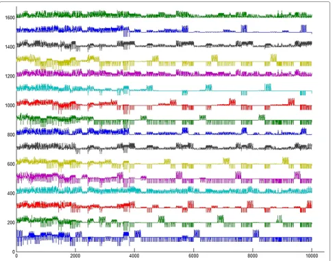
In order to prove noise robustness, input spike trains were corrupted by randomly inverting the state of 5% from all spike trains. Thus, some spikes were missing and some other random spikes were injected into the spike trains. Five training epochs were run before the evaluation. The implemented network successfully learned all patterns. In Figure 9, the membrane potential change is shown, hav-ing small values at the beginnhav-ing. Durhav-ing the trainhav-ing, the membrane potential becomes more and more polarized with strong negative values on the classes that are not rec-ognized by the selected neuron. It can also be appreciated that six neurons (numbered 8,10,13,14,15,16) remained almost untrained, with random weights.

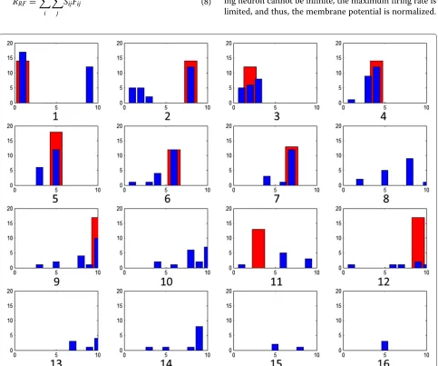
Training evolution can be observed by the spike rate diagrams shown in Figure 10. Each graph represents one neuron, with classes along X axis. Before training, every neuron is firing in several classes, and after the train-ing, each neuron has a discriminative high spike rate only in one class. As a result, the final weight maps of neu-rons become similar to the presented stimuli as Figure 11 depicts. The successful separation of patterns 2 to 5 and 1 to 6 proves that a network can solve problems with partially overlapping classes. The performance of learn-ing between classic SRM and simplified SRM models can be measured with the mean square error (MSE) for nor-malized weights after training. The training error for a single pattern (class 0) can be seen in Figure 12. The graph shows very similar learning dynamics and performance of both models. Starting from 5,000 TU, both models tend to increase the error showing over-training.

For comparing time of simulation, three synthetic datasets from Semeion samples with 5, 6 and 12 classes were prepared (12 classes dataset as digits 1 and 0 were represented with 2 classes each). Every class was repeated 30 times to test different network sizes (8, 9, 16 and 50 SNN neuron size in hidden layer were tested). Time of Matlab simulation in Table 1 shows an improvement over 20 times when comparing the simplified and classic SRM.

Simulation was done on a 64-bit OS system with 6 GB of RAM and an Intel i7-2620M processor.

6 Conclusions

In this paper, we describe a simplified spiking neuron architecture optimized for embedded systems implemen-tation, proving the learning capabilities of the design. The network preserves its learning and classification prop-erties while computational and memory complexity is reduced dramatically - by eliminating the PSP table in each neuron. Learning is stable and robust, the trained network can recognize noisy patterns. A simple, yet effec-tive visual input encoding was implemented for this net-work. The simplification is beneficial for reconfigurable hardware systems, keeping generality and accuracy. Fur-thermore, slight modifications would allow to be used with Address-Event Representation (AER) data protocol for frameless vision [29]. The proposed system could be further implemented in FPGAs for low-power embedded neural computation.

Competing interests

The authors declare that they have no competing interests.

Authors’ contributions

All authors are with Digital Signal Processing Group, Electronic Eng. Dept., ETSE, University of Valencia. Av. Universitat s/n, 46100 Burjassot, Spain.

Received: 30 April 2014 Accepted: 28 January 2015

References

1. Lovelace JJ, Rickard JT, Cios KJ. A spiking neural network alternative for the analog to digital converter. In: Neural Networks (IJCNN), The 2010 International Joint Conference On. New Jersey, USA: Institute of Electrical and Electronics Engineers-IEEE; 2010. p. 1–8.

2. Ambard M, Guo B, Martinez D, Bermak A. A spiking neural network for gas discrimination using a tin oxide sensor array. In: Electronic Design, Test and Applications, 2008. DELTA 2008. 4th IEEE International Symposium On. New Jersey, USA: Institute of Electrical and Electronics Engineers-IEEE; 2008. p. 394–397.

3. Bouganis A, Shanahan M. Training a spiking neural network to control a 4-dof robotic arm based on spike timing-dependent plasticity. In: Neural Networks (IJCNN), The 2010 International Joint Conference On. New Jersey, USA: Institute of Electrical and Electronics Engineers-IEEE; 2010. p. 1–8.

4. Alnajjar F, Murase K. Sensor-fusion in spiking neural network that generates autonomous behavior in real mobile robot. In: Neural Networks, 2008. IJCNN 2008. (IEEE World Congress on Computational Intelligence). IEEE International Joint Conference On. New Jersey, USA: Institute of Electrical and Electronics Engineers-IEEE; 2008. p. 2200–2206. 5. Perez-Carrasco JA, Acha B, Serrano C, Camunas-Mesa L,

Serrano-Gotarredona T, Linares-Barranco B. Fast vision through frameless event-based sensing and convolutional processing: Application to texture recognition. Neural Networks IEEE Trans. 2010;21(4):609–620. 6. Botzheim J, Obo T, Kubota N. Human gesture recognition for robot

partners by spiking neural network and classification learning. In: Soft Computing and Intelligent Systems (SCIS) and 13th International Symposium on Advanced Intelligent Systems (ISIS), 2012 Joint 6th International Conference On. New Jersey, USA: Institute of Electrical and Electronics Engineers-IEEE; 2012. p. 1954–1958.

(11)

Neural Networks (IJCNN). New Jersey, USA: Institute of Electrical and Electronics Engineers-IEEE; 2011. p. 880–885.

8. Fang H, Wang Y, He J. Spiking neural networks for cortical neuronal spike train decoding. Neural Comput. 2009;22(4):1060–1085.

9. Gerstner W, Kistler WM. Spiking Neuron Models: Single Neurons, Populations, Plasticity. Cambridge, United Kingdom: Cambridge University Press; 2002, p. 494.

10. Arguello E, Silva R, Castillo C, Huerta M. The neuroid: A novel and simplified neuron-model. In: 2012 Annual International Conference of the IEEE Engineering in Medicine and Biology Society (EMBC). New Jersey, USA: Institute of Electrical and Electronics Engineers-IEEE; 2012. p. 1234–1237.

11. Ishikawa Y, Fukai S. A neuron mos variable logic circuit with the simplified circuit structure. In: Proceedings of 2004 IEEE Asia-Pacific Conference on Advanced System Integrated Circuits 2004. New Jersey, USA: Institute of Electrical and Electronics Engineers-IEEE; 2004. p. 436–437.

12. Lorenzo R, Riccardo R, Antonio C. A new unsupervised neural network for pattern recognition with spiking neurons. In: International Joint Conference on Neural Networks, 2006. IJCNN 06. New Jersey, USA: Institute of Electrical and Electronics Engineers-IEEE; 2006. p. 3903–3910. 13. Painkras E, Plana LA, Garside J, Temple S, Galluppi F, Patterson C, Lester

DR, Brown AD, Furber SB. Spinnaker: A 1-w 18-core system-on-chip for massively-parallel neural network simulation. IEEE J. Solid-State Circuits. 2013;48(8):1943–1953.

14. Schemmel J, Grubl A, Hartmann S, Kononov A, Mayr C, Meier K, Millner S, Partzsch J, Schiefer S, Scholze S, et al. Live demonstration: A scaled-down version of the brainscales wafer-scale neuromorphic system. In: 2012 IEEE International Symposium on Circuits and Systems (ISCAS). New Jersey, USA: Institute of Electrical and Electronics Engineers-IEEE; 2012. p. 702–702.

15. Hylton T. 2008. Systems of neuromorphic adaptive plastic scalable electronics. http://www.scribd.com/doc/76634068/Darpa-Baa-Synapse. 16. Schoenauer T, Atasoy S, Mehrtash N, Klar H. Neuropipe-chip: a digital

neuro-processor for spiking neural networks. Neural Networks, IEEE Trans. 2002;13(1):205–213.

17. Schrauwen B, Campenhout JV. Parallel hardware implementation of a broad class of spiking neurons using serial arithmetic. In: Proceedings of the 14th European Symposium on Artificial Neural Networks. Evere, Belgium: D-side conference services; 2006. p. 623–628.

18. Rice KL, Bhuiyan MA, Taha TM, Vutsinas CN, Smith MC. Fpga implementation of izhikevich spiking neural networks for character recognition. In: International Conference on Reconfigurable Computing and FPGAs, 2009. ReConFig 09. New Jersey, USA: Institute of Electrical and Electronics Engineers-IEEE; 2009. p. 451–456.

19. Xilinx. Spartan-6 family overview. Technical Report DS160, Xilinx, Inc. October 2011. http://www.xilinx.com/support/documentation/ data_sheets/ds160.pdf.

20. Maass W. Networks of spiking neurons: The third generation of neural network models. Neural Networks. 1997;10(9):1659–1671.

21. MCWV Rossum, Bi GQ, Turrigiano GG. Stable hebbian learning from spike timing-dependent plasticity. J. Neurosci. 2000;20(23):8812–8821. 22. Pham DT, Packianather MS, Charles EYA. A self-organising spiking

neural network trained using delay adaptation. In: Industrial Electronics, 2007. ISIE 2007. IEEE International Symposium On. New Jersey, USA: Institute of Electrical and Electronics Engineers-IEEE; 2007. p. 3441–3446.

23. Paugam-Moisy H, SM Bohte. Computing with Spiking Neuron Networks In: G Rozenberg, JK T Back, editors. Handbook of Natural Computing. Heidelberg, Germany: Springer; 2009.

24. Booij O. Temporal pattern classification using spiking neural networks. (August 2004). Available from http://obooij.home.xs4all.nl/study/ download/booij04Temporal.pdf.

25. Bi G-Q, Poo M-M. Synaptic modifications in cultured hippocampal neurons: dependence on spike timing, synaptic strength, and postsynaptic cell type. J. Neurosci. 1998;18(24):10464.

26. Martinez LM, Alonso J-M. Complex receptive fields in primary visual cortex. Neuroscientist: Rev. J Bringing Neurobiology, Neurology Psychiatry. 2003;9(5):317–331. PMID: 14580117.

27. Foldiak P, Young MP. The Handbook of Brain Theory and Neural Networks. Cambridge, MA, USA: MIT Press; 1998, pp. 895–898. http://dl.acm.org/citation.cfm?id=303568.303958.

28. Repository UML. Semeion Handwritten Digit Dataset. 2014. http://archive. ics.uci.edu/ml/datasets/Semeion+Handwritten+Digit Accessed 2014-10-30.

29. Perez-Carrasco JA, Zhao B, Serrano C, Acha B, Serrano-Gotarredona T, Chen S, Linares-Barranco B. Mapping from frame-driven to frame-free event-driven vision systems by low-rate rate coding and coincidence processing–application to feedforward convnets. Pattern Anal. Machine Intelligence, IEEE Trans. 2013;35(11):2706–2719.

Submit your manuscript to a

journal and beneﬁ t from:

7Convenient online submission 7Rigorous peer review

7Immediate publication on acceptance 7Open access: articles freely available online 7High visibility within the ﬁ eld

7Retaining the copyright to your article