R E S E A R C H
Open Access
Linking demyelination to compound action
potential dispersion with a
spike-diffuse-spike approach
Richard Naud
1,2*and André Longtin
2*Correspondence:
1Ottawa Brain and Mind Research Institute, Department of Cellular and Molecular Medicine, University of Ottawa, Ottawa, Canada 2Department of Physics, University of Ottawa, Ottawa, Canada
Abstract
To establish and exploit novel biomarkers of demyelinating diseases requires a mechanistic understanding of axonal propagation. Here, we present a novel computational framework called the stochastic spike-diffuse-spike (SSDS) model for assessing the effects of demyelination on axonal transmission. It models transmission through nodal and internodal compartments with two types of operations: a
stochastic integrate-and-fire operation captures nodal excitability and a linear filtering operation describes internodal propagation. The effects of demyelinated segments on the probability of transmission, transmission delay and spike time jitter are explored. We argue that demyelination-induced impedance mismatch prevents propagation mostly when the action potential leaves a demyelinated region, not when it enters a demyelinated region. In addition, we model sodium channel remodeling as a homeostatic control of nodal excitability. We find that the effects of mild demyelination on transmission probability and delay can be largely
counterbalanced by an increase in excitability at the nodes surrounding the demyelination. The spike timing jitter, however, reflects the level of demyelination whether excitability is fixed or is allowed to change in compensation. This jitter can accumulate over long axons and leads to a broadening of the compound action potential, linking microscopic defects to a mesoscopic observable. Our findings articulate why action potential jitter and compound action potential dispersion can serve as potential markers of weak and sporadic demyelination.
Keywords: Demyelinating diseases; Axonal propagation; Spike timing variability
1 Introduction
Axons are the only link between our brains and the external world. Whether through touch, smell or vision, all the information we have about the external world is channeled through bundles of axons. Similarly, our only mean to interact with the external world is to send muscle commands along another set of axons. Clearly, this link must be made as fast as possible and myelination has evolved to regulate axonal propagation, minimizing the ‘temps perdu’ as coined by von Helmholtz [1]. Given its essential role in brain function, it is perhaps not surprising that disorders of axonal myelination are linked to dramatic loss of function. It is not clear, however, how mild demyelination affects propagation along nerve bundles, since its effect on internodal transmission is subtle. To better understand how mild demyelination gives rise to the early symptoms of demyelinating diseases, one
approach is to build mathematical models of the axon and study the link between demyeli-nation patterns and axonal conduction properties [2–5].
Mathematical modeling of myelinated axons can be separated into two approaches. The first approach, pioneered by Fitzhugh (1961) [6], aims to determine the basic electrody-namic properties regulating the flow of charges along a myelinated membrane. The prop-agation dynamics between the nodes are encapsulated in a single equation called the cable equation, which can be solved either analytically or with numerical methods to obtain at-tenuation or filtering properties [7,8]. This approach is restricted to uniform segments; it cannot typically capture the inhomogeneous myelination, paranodes or the alternation of myelinated segments and spiking nodes of Ranvier. To capture these inhomogeneities, one uses a second approach called compartmental modeling, where the system is mod-eled using a large number of small, locally uniform segments. Simulating numerically the exchange of charges between segments with different dynamic properties has revealed the important roles of myelin morphology and nodal dynamics for the propagation of action potentials [4,9–12]. This has been the main method to address the effects of demyelination [2,3,5], ion-channel noise [13–16], and spike after-potential [4] on axonal propagation.
In the present article we consider a hybrid approach. We model sequentially the nodal action potential generation in a small locally uniform spiking compartment and the intern-odal propagation resulting from a cable equation. Inspired from recent work on stochas-tic integrate-and-fire models [17–24] and the spike-diffuse-spike model of dendritic spine activation [25], we develop here the stochastic spike-diffuse-spike model (SSDS). We use this framework to investigate the propagation along axons where the excitability of a node can be enhanced to compensate for demyelination. We will start by describing the model-ing framework and how it incorporates demyelination as well as homeostatic ion-channel re-insertion. The framework will then be simulated to estimate the effect of mild and spo-radic demyelination on features of propagation. We will compute delay and jitter of action potential propagation first across a single node and then along a long axon. In addition, we will compute these metrics in the presence of homeostatic regulation of nodal excitability. Finally, we will use these estimates to compute the width of a compound action potential in various demyelination conditions. Potentially an early marker of demyelinating diseases [26–28], our results articulate how weak and sporadic axonal damage affect the delay and dispersion of the compound action potential.
2 Methods
The goal of this section is to expose the computational framework. First, we describe SSDS and use it to calculate analytically multiple quantities of interest: conduction speed, con-duction probability and spike timing jitter. Once the basic propagation model is outlined, a model of demyelinating damage articulates how this damage influences conduction speed, probability and jitter. Subsequently, the properties derived herein form the basis of the propagation along an axon bundle. We relate the single axon model to the characteristics of the compound action potential last.
2.1 Single axon model: stochastic spike-diffuse-spike.
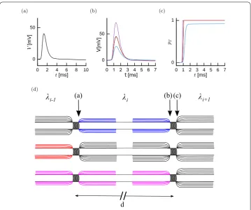
Figure 1The Stochastic Spike-Diffuse-Spike Model. (a) The action potential shape as it leaves the Ranvier node, schematically indicated in (d). (b) Propagation through the next internode alters the action potential shape as it reaches the next node (black, almost confounded with red). Damage to the internodes will affect this propagation following one of three possibilities. We consider whether demyelination affects the orthodromic internode only (purple), the antidromic internode only (blue) or both internodes equally (red). (c) Probability of transmission as a function of time for the intact and the three cases of damage. (d) Schematic illustration of two Ranvier nodes separated by a distancedfor the three damage configurations. For a propagation from left to right, we consider three possibilities for an action potential starting at node (a). Top: demyelination of orthodromic internode. Middle: demyelination of antidromic internode. Bottom: equal demyelination of both anti- and orthodromic internodes
compartment with no spatial extent and the internodal segment is modeled by a passive compartment with spatial extent. This modeling framework has been introduced previ-ously for active dendritic spines scattered along a dendrite [25]. Here we extend this mod-eling framework to capture axonal properties with the use of kernel-based methods. The two steps are described mathematically as
1. Internodal Drift Diffusion. Given an action potential leaving a node (Fig.1(a)), the charges entering and leaving the axon at the node will propagate along the
myelinated internodal region to the next Ranvier node. This operation is calleddrift diffusionbecause a large and succinct current in one node will be felt as a weaker and longer-lasting depolarization at the next Ranvier node, similar to the time evolution of molecules in water in the presence of a drift. At the location of the next Ranvier node, the result of this operation is depolarization of the membrane potential (Fig.1(b)).
We alternate steps (1) and (2) to reproduce the process of saltatory conduction. In the fol-lowing, we describe each of these steps in detail, along with the rationale for our modeling choices. For clarity of exposition, our simplifying assumptions are summarized here:
1. Action potential shape is invariant. Widening and shortening of action potentials produced at high frequency is therefore not captured by our present model. 2. Axons are modeled as a single thread. Reflection and impedance mismatch at
bifurcations would require extensions to the present model.
3. The electric coupling between nodes is restricted to pairs. For real axons, however, nodal spiking has a small but systematic effect multiple internodes away.
4. Propagation of current along an internode follows an idealized, semi-infinite, uniform cable. Taking into account the impact of peri-nodal structure and other types of inhomogeneous myelination would require a modification of the model. We have assumed a lumped compartment at the origin, composed of a Ranvier node and the antidromic compartment assumed to remain isopotential.
5. Demyelination can be modeled by changes in the electrotonic length constant.The electrotonic length constant is the distance over which a depolarization has decayed by a factor ofe–1, at steady state. Myelin greatly increases this length constant. The effects of demyelination on other parameters—such as the membrane time constant—are assumed to play a much weaker role [29].
2.1.1 Internodal drift diffusion
We want to relate the current associated with a spikeleavinga nodeIAP(t) (Fig.1(a)) to the membrane potential that this action potential causes in thenextRanvier node (Fig.1(b)). The effect of charged molecules drift-diffusing along the cable with potential leak across the membrane is captured by a convolution ofIAP(t) with the Green’s function, or impulse-response function of the internodal region. The Green’s function takes into account the dy-namics of the cable as well as possible impedance mismatch of the paranodal regions. Al-though the Green’s function is typically defined for all points in space, we are interested in the membrane potential at the location of the next node. Assuming that the orthodromic position from nodeican be parameterized by a single coordinateX, we letGi(T,X) be the
Green’s function of theith internodal region. Accordingly, we can compute the membrane potential along theith internodeVi(T,X) with origin at theith Ranvier node as
Vi(T,X) =
∞
0
Gi
T–T,XIAP
TdT, (1)
whereX=x/λiis a unitless variable for the distancexalong the axon in units of the
elec-trotonic length of the orthodromic internodeλi.T =t/τ a unitless variable for time in
units of the membrane time constantτ. We also note thatVi corresponds to distance
from resting potential, such that resting potential isV = 0 mV and the action potential threshold isV= 20 mV.
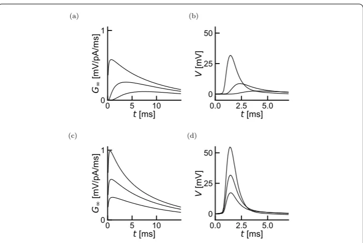
Figure 2Impulse Response function for internodal current propagation. (a) The impulse-response function of a semi-infinite cable with lumped soma is shown for increasing effective distancesX= 0.1, 0.5, 1 (from top to bottom) forγ= 1. (b) A typical action potential current filtered with the Impulse-response function shown in (a). (c) Impulse-response function of a semi-infinite cable with lumped soma for increasing electrotonic ratiosγ= 2, 1, 0.5 (from top to bottom) andX= 0.1. (d) Membrane potential obtained by filtering the action potential current with the Green’s functions shown in (c)
a compartment lumped at the origin of the cable. This expression was derived for propa-gation of charges in a uniform semi-infinite and passive dendrite with a somatic compart-ment lumped at its base [33]. The assumptions underlying this derivation are also satisfied by the axon leaving a leakier Ranvier node. The Green’s function is thus parameterized by a single parameterγi,i–1> 0 (see below) relating the impedance mismatch between the lumped compartment and the cable [33]
Gi(T,X) =γi,i–1eγi,i–1X+(γ
2
i,i–1–1)Terfc
γi,i–1 √
T+√X 4T
(2)
valid forT> 0,X> 0. The lumped compartment encapsulates a dependency on the state of the antidromic internode (Fig.1(d)). Figure2illustrates how this Green’s function depends onX,T andγ.
In Eq. (2), we have usedX, the internodal distance, in units of the electrotonic length constantλ. The location of the next node is therefore the unscaled internodal distanced
divided by the distanceλover which a steady state depolarization has fallen by a factore–1 in the orthodromic compartment, such that
D= d λi
. (3)
In what follows we will focus on the position of nodei+ 1 using the nodeias reference,
X=Dand the position of nodeiin the same reference systemX= 0.
or-thodromic compartmentraλi[33,34]. If the lumped compartment has a total resistance
corresponding to the sum of the axial resistance over one electrotonic length of the an-tidromic axonraλi–1and the much smaller transmembrane resistance of the Ranvier node,
RN, then we obtain the simple relation
γi,i–1=
raλi–1+RN
raλi ≈
λi–1 λi
. (4)
For the Green’s function of theith internode, the parameterγ is the electrotonic length of the antidromic compartmentλi–1 divided by that of the orthodromic compartment λi.
For an intact axon the electronic constant of successive internodes is uniform λi–1 = λi ≡ λM and γ = 1, where λM is the electrotonic constant of a fully myelinated
in-ternode. Similarly, for a fully demyelinated axon, the electrotonic constant is uniform andγ = 1. Uneven myelination will affectγ such that orthodromic demyelination im-plies γ > 1 (top in Fig. 1(d)) and antidromic demyelination implies γ < 1 (middle in Fig.1(d)).
The only parameters regulating internodal filtering are, therefore, the membrane time constantτ, the internodal distancedand the orthodromic and antidromic electrotonic constants,λiandλi–1, respectively. In the following, the membrane time constant is set to a typical valueτ = 15 ms. In addition, we used an internodal distanced= 1 mm con-sistent with experimental recordings [35]. The myelinated electrotonic constant is cho-sen to be much larger than the internodal distance to ensure rapid propagation. We used λM = 200 mm as a baseline electrotonic constant for a fully myelinated
intern-ode.
2.1.2 Nodal spiking
Given a membrane potential time course from the drift-diffusion step,Vi, we now calculate
a probability of firing associated with this depolarizing drive. Nodal spiking is considered to be probabilistic since it results from the stochastic activation of a finite number of ion channels [13,36,37] amid disturbances from ephaptic coupling with neighboring axons [38–42]. To capture this stochasticity, we use a common approximation where all noise sources can be encapsulated in a simple mapping between a deterministic membrane po-tential driveVi(T,X) and a probability intensity, or hazard,ρi+1(T) [21,43,44]. Following previous theoretical and experimental estimates of this hazard [45,46], we assume that ρ is determined by an exponential function of the membrane potential. How the firing probability depends on the rate of change of the membrane potential can be included in the formalism at a later time [45]. In our model, the probability intensity is high when the membrane potential is above a fixed thresholdθ and goes smoothly to zero when it is below. Using a scaling factorβwe can write the probability intensity time course for the membrane potential time courseVi(T,X) as
ρi+1
Vi(T,X)
=ρ0exp
βVi(T,X) –θ
, (5)
nonlinear relationship between membrane potential and probability of firing is thought to reflect the fact that noise may cause the neuron to fire as a function of the separation between the instantaneous voltage and the voltage threshold. This model is known as the spike-response model with escape noise [21,44]. It has been successfully applied to exper-iments on cortical neurons. Given the relatively similar kinetics between action potential generation in the axon hillock and action potential generation in the Ranvier nodes, we believe that the accuracy previously shown for the soma-hillock [20] will apply also to the Ranvier Nodes. In sum, the hazard function in Eq. (5) specifies the firing intensity of an inhomogeneous Poisson process.
This probability intensity is used to define the probability of transmission (Fig.1(c)). Using the hazard-function formalism [21], we consider the probability that a spike will have been transmitted between time zero and timeT:
pi+1(T) = 1 –e–
T
0 ρ(Vi(s,X))ds, (6)
where we have omitted the dependency onXfor simplicity of notation. We note that this expression implies a nonlinear transformation from the membrane potential time course to the probability of firing.
The probability of transmissionPT(i+1)(λi,γi,i–1) follows as might be expected from this quantity: it is the probability that a spike will have been transmitted after a sufficiently long time,PT(i+1)=pi+1(t∗/τ). We usedt∗= 10 ms throughout our work, which is much larger than the time taken to travel between two nodes.
To ensure realistic dynamics, we calibrated the parameters of the model,β,θ andIAP, on publicly available data as follows. For the action potential time courseIAP, we used membrane potential recordings from deep cortical neurons of young rats [47] stimulated with time-dependent current-clamp input. To extract the current time course from the membrane potential time course, we computed the first derivative of the spike-triggered average. This current time course is used as a template current leaving any given internode (Fig.1(a)). We have chosenβ= (5 mV)–1 to obtain a threshold variability as previously reported for human axons [13]. We chose the action potential threshold θ in order to obtain a physiological propagation delay given our choice of electrotonic constants, as described in the next section.
2.1.3 Internodal delay and speed
To determine the propagation speed, we consider a spike leaving nodei and traveling toward the next node,i+ 1, through internodei. The propagation speed will then be ex-pressed as a function of the internodal delay and the internodal distance. Inhomogeneities in internodesj>ican in principle affect the delay involved in crossing internodei. These effects are neglected here, but they could be incorporated by using compartmental mod-eling to calibrate the impulse-response function for all possible states of the downstream internodes.
The membrane potential at internodei+ 1, which in our notation is the voltage at the previous node propagated over a distanced, i.e.Vi(T,D(λi)), is obtained from Eq. (1) with
λibeing the electrotonic length constant of internodeiandγi,i–1=λi–1/λicharacterizes
(Eq. (4)). Using the firing intensity defined in Eq. (5), we can obtain the probability that the first spike occurs at timeT[21]:
Pi+1(T,X) =ρi+1
Vi(T,X)
e– 0Tρi+1[Vi(s,X)]ds, (7)
where we make explicit the dependence onVi(T,X) through Eq. (5).
The internodal delay is the difference between the time at which the spike is produced at nodei,Ti∗and the time at which the spike is produced at nodei+ 1,Ti∗+1, namely
δTi=Ti∗+1–Ti∗. (8)
The timing of a spike at internodei+ 1 is taken to be the maximum likelihood timing
Ti∗+1=argmaxPi+1
T,D(λi)
=argmaxρi+1
Vi(T,D(λi)
e– 0Tρi+1[Vi(s,D(λi)]ds. (9)
To compute the reference spike timeTi∗, we use the membrane potentialVi–1calculated withγ = 1 in Eq. (1) andλM:
Ti∗=argmaxPi+1(T, 0) =argmaxρ
Vi(T, 0)
e– 0Tρ[Vi(s,0)]ds. (10)
Together, these quantities are used to calculate the propagation speedviacross internode
i, that is, the internodal distanceddivided by the internodal propagation delay
vi= d τ δTi
. (11)
Figure3shows how the membrane potentials atiandi+1 (Fig.3(a)) lead to a propagation speed (Fig.3(b)). This speed depends on the length constantsλiandλi–1as well as on the thresholdθ. Increasing the threshold in Eq. (5) broadens the first-spike time distribution and increases the delay (Fig.3(c) and (d)). For a uniform myelination withλi=λi–1=λM=
20 mm, we haveγi,i–1= 1 andX= 0.005. The small effective distance leads to a small shift of the membrane potential atX= 0 to the membrane potential atX= 0.005 (Fig.3(a)). We can compute the speed for a given value of the thresholdθ. The propagation speedv
decreases as the threshold is increased (Fig.3(b)).
We use this relationship to determine a threshold that gives realistic propagation speeds. Specifically, we numerically calculate the speedv(θ) for every value of the thresholdθand find the thresholdθ∗for whichv(θ∗) is close to 80 m/s. This is obtained for a threshold at θ= 20 mV, corresponding to the typical separation between resting and threshold poten-tial.
2.1.4 Homeostatic threshold compensation
Figure 3Propagation Speed. Notice that the time scales are in milliseconds. (a) Filtered action potentials at distanceX= 0 (red) andX= 0.005 (black), corresponding tod= 1 mm andλM= 200 mm. The threshold is
shown in blue. Inset expands area in the gray rectangle. (b) The resulting speed of propagation (Eq. (11)) as a function of thresholdθ. The blue dashed line indicatesθ∗, the parameter value used in the simulations. An average transmission delay of 0.0125 ms overd= 1 mm yields a speed of 80 m/s. (c) Difference between latency distributions calculated from the action potential atX= 0 andX= 0.005 (shown in (a)) forθ= 20 mV. Inset expands area in the gray rectangle. (d) Same as (c) butθ= 50 mV
2.1.5 Jitter
The variability of propagation delay is quantified by the standard deviation of δTi.
Ac-cordingly, we want to estimateσi+1andσi, the standard deviation characterizing the
de-lay distributionPi+1(T) andPi(T), respectively. These standard deviations are estimated
numerically from the full width at half maximum (FWHM) ofPi+1(T) andPi(T), using
σi+1= FWHM[Pi+1]/2.35, and similarly forσ0. A Gaussian approximation on the latency distributionsPi+1(T) andPi(T) means that the jitter associated with an intervalican be
computed from
σi=
σi2+1+σi2. (12)
2.2 Modeling axonal damage
We consider demyelinating damage. Demyelination is modeled in SSDS as an alteration to the drift-diffusion step.
2.2.1 Altered propagation
Demyelination will affect the three principal passive cable properties differently: the relax-ation time constantτ, the electronic lengthλand the resistance ratioγ in Eq. (1). Firstly, the time constant is a product of transverse resistance in an internodal region RT and
compartment capacitanceC,τ =RTC. When an internode undergoes demyelination, its
transverse resistance is assumed to increase while its capacitance decreases [29]. There-fore, the time constant may remain approximately constant under demyelination.
On the other hand, the electronic length is given byλ2=R
T/Ra whereRa is the axial
the axial resistance, the electrotonic length will decrease. Therefore, we argue that the effect of internode demyelination is to increase the effective internodal distance through a reduction of the electrotonic length.
The resistance ratioγ parameterizes the effect of a mismatch between resistance of an-tidromic and orthodromic internodal regions. We will denote the different configurations with four cases for the value ofγi,i–1.γ11corresponds to the intact axon (λi=λi–1=λM),γ10 to antidromic damage (λi–1=λD),γ01to orthodromic damage (λi=λD) andγ00to damage on both internodes (λi=λi–1=λD). Thus, when both internodal regions are intact or when
both internodal regions are equally demyelinated, we haveγ11=γ00= 1. When only one of the internodal regions is intact, we expectγ10< 1 for antidromic demyelination and, con-versely,γ01> 1 for orthodromic damage. Sinceγ modifies multiplicatively the current in Eq. (1), this is consistent with a greater net axial current flowing orthodromically from the Ranvier node forγ01, and conversely forγ10. Our computational work reveals in fact that the current flowing orthodromically from the spiking node will leak out of the reduced membrane resistance there, potentially making it weaker at the next node (Eq. (2)). How-ever, the current flowing antidromically will also be relatively smaller, due to the higher resistance added by the intact myelin. The result is an extra orthodromic contribution that more than compensates the first effect.
To model the effect of demyelination on the electronic length and the resistance ratio si-multaneously, we suppose that the unmyelinated, or maximally demyelinated, fiber has an electronic lengthλL. This will serve as a lower bound. Similarly, the intact internode has
an electrotonic lengthλM. A demyelinated internodal region is associated with an
elec-trotonic lengthλDbetweenλLandλM. Demyelination will reduce the effective internodal
distanceXfromd/λMtod/λD. Concurrently, it will modify the resistance ratio according
toγ10=γ01–1=λD/λM, withγ00andγ11unchanged.
Given this parameterization of damage in terms of the electrotonic length, we quantify the intensity of damage by its relative change inX:
Damage = 1 – λD–λL λM–λL
. (13)
This metric, reported in percent, takes a value between 0% and 100%. We say that dam-age is maximal when the intensity of damdam-age reaches 100%. We use a typical value of λL= 1 mm for the fixed unmyelinated length constant [48]. Although modern estimates
of this length constant in the cortex are about half this value [49], the results presented here do not critically depend on this lower bound. For the fully myelinated space constant we chooseλM=200 mm.
2.2.2 Delay,failure and jitter along a complete axon
We will calculate the propagation statistics in terms of four numbers: 1) the number of damaged internodes preceded by an intact internodeN10, the number of damaged intern-odes preceded by a damaged internodeN00, the number of intact internodes preceded by an intact internodeN11, and the number of intact internodes preceded by a damaged in-ternodeN01. The total number of nodes is simply the sum of the number of each type of internode:
N=
i,j
The total probability of transmission is the product of all internodal transmission prob-abilities:
P(axon)T = 1
i=0 1
j=0
PT(i)(λi,γij)Nij. (15)
We wish to calculate the distribution of delays for a spike traveling along a complete axon, given a pattern of demyelination determined by the number of nodes in each of the four categoriesN00,N01,N10andN11. Although it is possible to compute this distribution with nested convolutions of the internodal delay distributions, we will assume that each internodal delay distribution is well captured by a Gaussian. Then the delay for the whole axon is the weighted sum of the delay associated with each type of internodes
δTN=
1
i=0 1
j=0
NijδT(λi,γij). (16)
Similarly, the jitter is obtained by the weighted sum of the single internode variances.
σN2= 1
i=0 1
j=0
Nijσ(λi,γij)2. (17)
The Gaussian approximation holds well as long as the membrane potential crosses the stochastic threshold. This gives delay distributions that are sharp and approximately sym-metric.
2.2.3 Modeling damage distribution
Here we consider a simple model where lesion can occur with constant probabilitypLand
when a lesion occurs, it creates a damage in a fixed number,k= 1, 2, 3, . . . , of successive internodes. When an internode is damaged its electrotonic length is reduced by a fixed amount that is the same for all lesions. This model is an approximation of the complex mechanisms giving rise to a correlation between the damages at subsequent internodes [50].
The parameterskLandpdetermine how theNijare randomly generated. First we
gen-erate the number of lesions using a binomial distribution,NL∼Binom(N,pL):
p(NL) =
N NL
pNL
L (1 –pL)N–NL, (18)
whereNis the mean total number of internodes.
It follows that the number of nodes situated at the leading edge of a lesionN01will equal the number of lesions,NL, unless a lesion is situated at the end of the whole axon. Similarly,
the number of nodes situated at the trailing edge of a lesionN10will equal the number of lesionsNLunless a lesion is situated at the very beginning of the whole axon. For simplicity
we take,N01=N10=NL. The number of nodes surrounded by two damaged internodes,
N00, is zero if lesions consist of isolated internodes (k= 1). Otherwise, fork> 1, we have
Eq. (14):N11=N–NL(k+ 1) fork> 1 andN11=N– 2NLfork= 1. Here the total number
of internodesNis not a fixed number but a function of the random numberNL(Eq. (14)).
In the regimekandpL1, the fluctuations ofNaroundNwill be relatively small.
The average number of lesion that results from this scenario isNL=NpL.
The overalltemps perdu,TP, averaged over the lesion configuration thus becomes a function of the average number ofNL,
TP(NL) =
1
i=0 1
j=0
Nij(NL)
δT(λi,γij) (19)
and similarly for the variance,
σTP2 (NL) =
1
i=0 1
j=0
Nij(NL)
σ(λi,γij)2. (20)
Together Eqs. (19)–(20) describe a Gaussian approximation to the spike time distribution at the end of an axon.
2.3 Compound action potential
Previous theoretical investigations [51,52] have concluded that the local field potential (LFP) can be well captured by monopole terms for the current sources. For myelinated nerves, current sources consist mostly of the transmembrane currents underlying the ac-tion potential generaac-tion at the nodes of Ranvier. The LFP is then obtained by summing the contributions of each node of Ranvier in the proximity to the recording electrode. Given a relatively large internodal distance, only the nodes closest to the recording electrode will contribute to the LFP. We can therefore sum for each axonlonly the contribution of the nearest node. Let the electrode be closest to thenth node of each axon, and write the current of the nearest node asIln(t) and its location with respect to the recording
elec-trode asrln. We have the electric potentialφarising from transnodal currents scaled by a
Coulombic factor:
φ(t) = 1 4π σe
L
l=1
Iln(t)
rln
, (21)
whereσeis the electric permittivity [51]. Equation (21) can be related to our framework
by considering that the current at timetin a given node is the action potential current triggered with a delayδTln:Iln(t) =IAP(t–δTln).
According to the law of large numbers, the sum of the distance-scaled nodal currents over a large number of independent and identically distributed currents should be close to their expected value. Also, since we are only interested in the relative amplitude of the compound action potential, we lump the scaling factors into a constantcand focus on the time-dependence. This scaling constant captures geometrical factors which will scale the LFP uniformly depending on the spatial distribution of the nearest nodes. We therefore obtain
φ(t) =c
where we have dropped the subscriptnfor simplicity. The compound AP is proportional to the convolution between the cross-membrane current during an action potential and the latency distribution of the nearest internode.
We apply the central-limit theorem to obtain the following form for the compound ac-tion potential:
φ(t) =c
IAP(t–δT)
PT(NL)F
TP(NL),σTP2 (NL)
dNLdδT, (23)
whereF(μ,σ2) is a normal distribution with meanμand varianceσ2. The mean and the variance are given by Eq. (19) and Eq. (20), respectively.
Following the Gaussian approximation of Eq. (16), the distribution of delays for propa-gation between node 0 and node N can be written as
P0:N(δT) =
PT(NL)F(μ,σ)p(NL)dNL (24)
and the number of lesions follows a binomial distribution (Eq. (18)). Taken together, Eqs. (23)–(18) determine the compound action potential. The main quantities of interest are listed in Table1. A summary of the steps used to compute the probability of
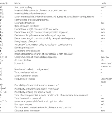
propa-Table 1 Glossary of parameters and variables
Variable Name Units
β Stochastic scaling mV–1
δTi Internodal delay in units of membrane time constant –
δTN Internodal delay for whole axon –
δTTP Mean internodal delay for whole axon and averaged across lesion configurations –
φ Normaliozed extracellular potential –
θ Stochastic threshold mV
γ Ratio of length constants –
λi Electrotonic length constant of ith internode mm
λM Electrotonic length constant of a myelinated segment mm
λD Electotonic length constant of a damaged segment mm
λL Electrotonic length constant of a fully demyelinated segment mm
ρi Firing hazard of nodei –
σ2
TP Variance of transmission delay across lesion configurations –
σe Electric permittivity –
τ Membrane time constant ms
D Internodal distance in units of electrotonic length constant –
Gi(T,X) Green’s function of internodal propagation mV / pA
IAP AP current influx pA
k Lesion size Number of
internodes
Nij Number of nodes in configrationij –
NL Total number of lesions –
N Mean number of lesions –
pL Frequency of lesions Lesions per
node
P(Ti) Probability of transmission across internodei –
P(Taxon) Probability of transmission across whole axon –
pi(T,X) Probability of firing first spike at nodei–
Ti Time of action potential in nodeiand in units of membrane time constant –
t Time from action potential ms
Vi(T,X) Membrane potential deflection along internodei mV
v Propagation speed m/s
X Distance along internode in units of electrotonic constant –
gation, jitter distributions and compound action potential is given in the first part of the Results section.
3 Results
In order to study how demyelination affects action potential transmission over long ax-ons, we constructed a computational model that captures the essential features of salta-tory propagation. The stochastic spike-diffuse-spike model (SSDS: see Methods) iterates between a stochastic firing step and a cable-filtering step. In the drift-diffusion step, fir-ing in nodei causes a membrane potential change in nodei+ 1 as determined by the cable impulse-response function. This step modifies the width and the amplitude of the action potential in a manner phenomenologically equivalent to drift diffusion. In the fir-ing step, we determine the firfir-ing probability given the membrane potential reachfir-ing this node. The biophysical mechanisms underlying stochastic firing are not specified in the SSDS but they are thought to reflect both the stochastic opening of possibly distinct types of voltage-dependent ion channels in the node of Ranvier [13,36,37,53] and the ephaptic couplings with neighboring axons [38–42]. Effects of specific biophysical noise sources on excitability could be approximated in this phenomenological formalism through ad-justments to the hazard function. This SSDS model allows us to estimate transmission probability, propagation delay and spike timing jitter for any axon length as a function of the number of damaged nodes.
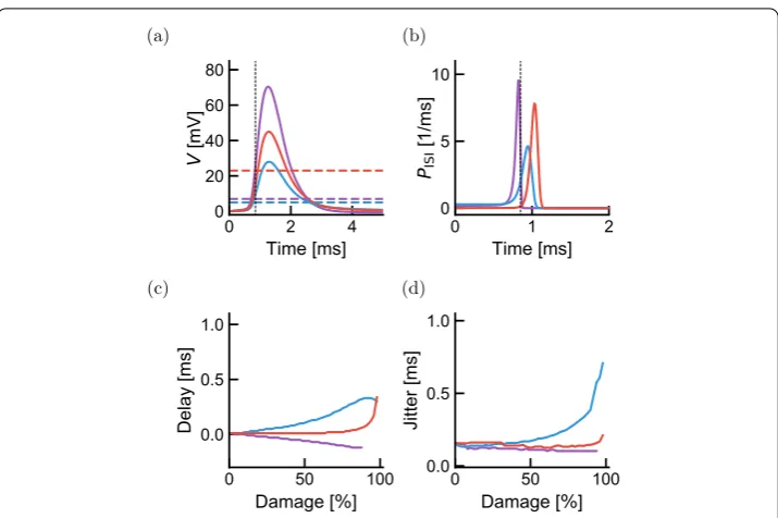
Figure1illustrates the SSDS model for three distinct local patterns of demyelination for a spike leaving a given node and propagating through the orthodromic internode to the next node. Upon activation of the first node of Ranvier, the stereotypical time course of the action potential is observed (Fig.1(a)). Depending on the demyelination pattern, the stereotypical current from the first node will produce a depolarization in the next node (Fig.1(b)). This depolarization time course is used to calculate the probability that an action potential is produced in this node (Fig.1(c)). Three distinct types of demyelination pattern are distinguished (Fig.1(d)): demyelination of the orthodromic internode only, demyelination of the antidromic internode only, and demyelination of both antidromic and orthodromic regions. If a spike is generated in the next node, the process continues along the axons iteratively.
Parameters of the SSDS consist of a non-parametric time-dependent current resulting from the stereotypical time course of ionic currents in the Nodes of Ranvier (IAP), the impulse-response function regulating propagation of this current to the next node of Ran-vier (GX), the firing threshold at the nodes (θ) and the stochastic firing sensitivity (β).
Demyelination will directly affect the impulse-response function. In fact we find that for our parameterization, two parameters regulate the shape of the impulse-response func-tion. For a nodeifollowed by internodeiand preceded by internodej, these two param-eters are the electrotonic length constant for the orthodromic cableλi and the ratio of
orthodromic and antidromic length constantsγij. Demyelination reduces the length
con-stant by an amount reflecting the degree of demyelination (see Methods). Figure2 illus-trates how the different filtering properties arise from changes in the electrotonic constant λikeeping the antidromic one fixed. Both the impulse-response function amplitude and
the temporal profile are affected by changes in the orthodromic length constant (Fig.2(a)). As a result, a decrease inλiwill produce both a dampening and a broadening of the
depo-larization reaching the next internode (Fig.2(b)). In contrast, modifying the antidromic-to-orthodromic ratio of length constantsγijwhile keeping the orthodromic electrotonic
length fixed modifies the amplitude of the impulse-response function without affecting its time course (Fig.2(c)). This results in a dampening of the depolarization reaching the next node, which is seen without an associated broadening (Fig.2(d)). Therefore our SSDS model is biophysically justified, and it can be used to understand how different demyeli-nation patterns relate to propagation properties.
3.1 Demyelination and propagation properties—single internode
To study the effects of demyelination on single internodal propagation, we derive expres-sions for propagation delay (Eq. (19)), spike timing jitter (Eq. (20)) and transmission prob-ability (Eq. (15)) in the SSDS model. We then study the effect of demyelination intensity for the three different damage patterns illustrated in Fig.1(d), namely damage affecting the orthodromic region, the antidromic region, or both regions with equal intensity. The degree of demyelination is quantified with a metric for quantifying damage (see Methods, Eq. (13)), which varies between 0% for intact internodes, and 100% for complete demyeli-nation.
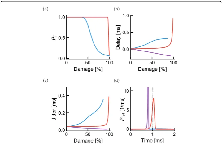
We find that transmission probability is only affected at extreme damage intensities for the uniform and orthodromic damage patterns (Fig.4(a)). This is consistent with previ-ous computational studies showing that a very high degree of demyelination is required to prevent internodal propagation [2,54,55]. When the damage is antidromic, however, the probability of transmission starts to drop sharply at mild damage intensities (60% damage). In the SSDS model, this effect results from the impedance imbalance, where an antidromic demyelination reduces the impedance in the antidromic direction. This reduces the net axial current flowing in the orthodromic direction and therefore prevents propagation. Consistent with this view, the delay and jitter both increase for weak demyelination inten-sities when the damage is antidromic (Fig.4(b) and (c)). In the case of uniform damage, increases in both the delay and the jitter are observed only for very large demyelination intensities.
Figure 4Effect of demyelination on propagation across a single internode. (a) Effect of demyelination on the probability of transmissionpTfor the three cases shown in Fig.1(purple is orthodromic damage, blue is
antidromic damage and red is damage on both sides of the node). A purple line is hidden behind the red curve, but stays atpT= 1 over the range of damage intensities studied. (b) Effect of demyelination on
transmission delay. Having negative delays means a propagation delay shorter than in the absence of damage. Delays corresponding topT< 0.1 are not plotted. (c) Same as (b) but for transmission jitter. (d) Spike
timing distributions corresponding to 80% damage (based on a time discretization of 0.01 ms)
than 50% damage), mild damage should cause a net increase in spike timing jitter whereas the net delay does not vary strongly with damage.
3.2 Lesion patterns and propagation properties—whole axon
We now turn to the demonstration of the power of the model to predict whole axon propa-gation properties. To determine how demyelination patterns affects propapropa-gation along the length of an axon, we consider demyelination in lesions made of segments ofkcontiguous internodes. Lesions are then assumed to arise randomly with probabilitypL. Transmission
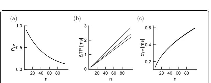
probability, propagation delay and spiking jitter are then computed analytically (see Meth-ods). For a fixed, mild degree of demyelination, increasing the lesion probability sharply decreased the probability of transmission over long axonal distances (50% damage,k= 1, Fig.5(a)). The total transmission delay increases linearly with distance, consistent with a constant but damage-dependent speed of propagation. Lesion probability strongly affects this effective propagation speed (Fig.5(b)). In contrast, the jitter increases sub-linearly with the number of internodes traveled (Fig.5(c)), consistent with a linear increase in vari-ance. These results suggest that lesion probability strongly affects propagation properties even for a mild degree of demyelination.
Figure 5Effect of lesion frequency as a function of the number of successive internodes. For a fixed lesion sizek= 1 and damage intensity 50% damage, the probability of transmission (a), the transmission delay (b) and the jitter (c) are shown as a function of the average total number of internodes. Lesion frequencies are plotted forpL= 0.01, 0.1, 0.2 (from bottom to top in panel (a) and from top to bottom in panels (b) and (c))
Figure 6Effect of lesion size as a function of the number of successive internodes. The setup is the same as for Fig.5, but for three lesion sizes:k= 1, 3, 7 (from bottom to top) and fixed lesion frequencypL= 0.1. Note
that the probability of transmission and the jitter depend very weakly on lesion size, as the lines perfectly overlap
antidromic internodes (Fig.1, red) without affecting the proportion of asymmetric dam-age configurations. Since symmetric damdam-age configuration affects propagation properties only at very strong demyelination degree (Fig.4, red curves), lesion size does not affect propagation properties at weak demyelination intensities.
3.3 Homeostatic control of demyelination-induced delays
Figure 7Homeostatic adjustment of threshold partially compensates for demyelination-induced delays and transmission probability across a single internode. For each demyelination intensity and depending on the antidromic-orthodromic location of the damage, we attempted to recover undamaged delays by adjusting the spiking threshold. (a) For 40% damage, the membrane potentials reaching the next node of Ranvier (full lines) are shown with their corresponding firing thresholds that minimize delay changes (dashed horizontal lines). (b) Delay probability distributions for the membrane potentials shown in (a). (c) The residual delay and (d) spike timing jitter are shown as a function of damage intensity. Colors follow the convention in Fig.1
to preserve the propagation speed. In order to model this homeostatic adjustment, we have replaced the fixed firing thresholdθ by a threshold adjusted to be the highest value that would preserve conduction velocity. This homeostatic compensation is limited in the model by restricting the adjustment range for the threshold (see Methods, Sect.2.1.4).
We start by considering the effect of homeostatic compensation on the propagation properties of a single internode. As expected from the observation that delays increase (decrease) when damage is antidromic (orthodromic) (Fig.4), the compensated threshold was low for the antidromic damage configuration, unchanged for the symmetric damage configuration and increased for the orthodromic damage configuration (Fig.7(a)). This homeostatic compensation ensured a high transmission probability even for severe de-myelination. Delays and jitters depend on damage configuration and intensity, in a manner that remains qualitatively identical to the absence of threshold compensation (compare Fig.7(c) and (d) with Fig.4(b) and (c)).
However, quantitatively the picture is very different. As imposed by homeostatic com-pensation, the delay across a single internode remained approximately constant for a larger range of damage intensities (Fig.7(c) and (d)). As the degree of demyelination increases, the change in threshold fails to compensate for this damage, with the result that both delay and jitter are affected.
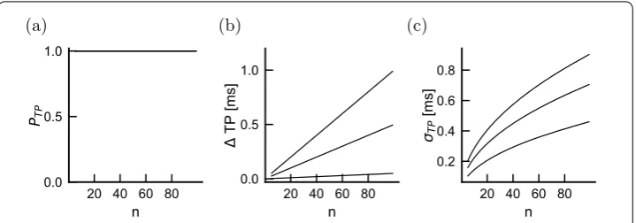
Figure 8Effect of lesion frequency over multiple internodes in the presence of homeostatic compensation. The probability of transmission (a), the transmission delay (b) and the jitter (c) are shown as a function of the number of internodes through which the activity propagates. Three lesion frequencies are plotted:pL= 0.01,
0.1, 0.2 (from bottom to top in panels (b) and (c), perfect overlap in panel (a)). The demyelination of each lesion corresponds to 50% damage
compensation. These observations suggests that the measurement of jitter could reveal demyelination, whether homeostatic compensation were at work or not.
To determine the effects of compensated demyelination on the whole axon, we deter-mine transmission probability, delay and jitter as a function of the total number of nodes (Fig.8). Similar to the case without homeostatic compensation, the propagation properties depend only weakly on the lesion size. We therefore focus on the effects of lesion probabil-ity. For mild damage intensities (50% damage), transmission is preserved even when lesion probability is 0.2 (Fig.8(a)). Propagation speed decreases with lesion probability, but de-lays remain 2–3 times smaller than in the absence of threshold compensation (Fig.8(b)). In comparison, although larger without compensation (Fig.4(c)), remain of the same or-der of magnitude as with compensation (Fig.7(d)). We conclude that spike timing jitter can be a good predictor demyelination frequency and intensity even when there is nodal excitability compensation.
3.4 Compensated demyelination can be inferred from the compound action potential
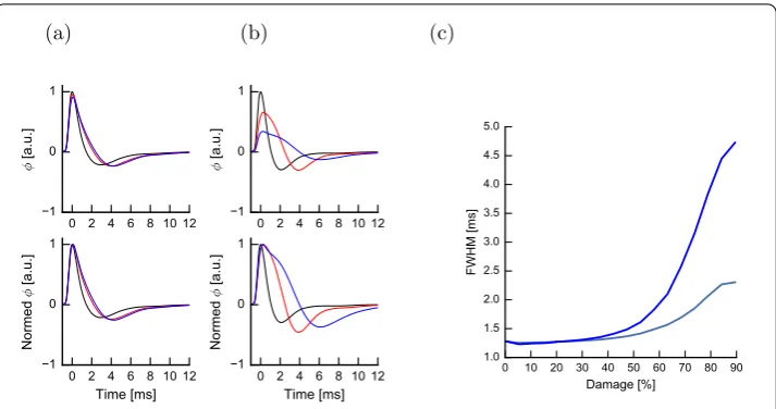
To investigate whether the effects of demyelination may be observed experimentally, we estimated the extracellularly recorded compound action potential expected from a bun-dle of simultaneously activated axons (see Methods, Eq. (23)). We illustrate our results in the context of homeostasis. We study the hypothesis that an increase in jitter, by reducing the synchrony within the bundle, may affect the width of the compound action poten-tial. Figure9(a) shows that mild (50% damage) lesion probability increases both the delay of the first trough and the width of the compound action potential. The propagation is strongly impeded by rare but severe (97% damage) lesions as revealed by the amplitude of the compound action potential (Fig.9(b)). Figure9(c) shows how the full width at half maximum (FWHM) has a clear dependence on both the damage intensity and the lesion frequencypL. We conclude that the width of the compound action potential, like the jitter
Figure 9Effect of lesion size and intensity on the compound action potential in the presence of threshold compensation. The compound action potential is shown (top) for an intact axon withN=100 internodes (black line) and two lesion frequenciespL= 0.01 (red) andpL= 0.2 (blue). Intensity of damage and lesion size
are kept fixed (50% damage,k= 1). The time course is normalized to the peak amplitude of intact axons (bottom). (b) Compound action potential for changing lesion intensity 70% damage (red) and 97% damage (blue) while keeping size and frequency of lesions fixed (pL= 0.1,k= 1). (c) The Full Width at Half Maximum
(FWHM) of the compound action potential as a function of damage intensity for rare and small lesions (gray,
pL= 0.1,k= 1) and frequent but small lesions (blue,pL= 0.2,k= 1)
4 Discussion
We have presented a modeling framework to estimate propagation delay and jitter in weakly or sporadically demyelinated axons. The framework extends the SSDS model of propagation along an unmyelinated dendrite with equally spaced excitable spines [25,62, 63] to the context of a myelinated axon with excitable nodes of Ranvier. Our goal is to account for different spike shapes and stochastic firing effects. The simplified computa-tional model can be used to simulate propagation over a very large number of nodes and internodes, and also to determine how weak or sporadic damage can cumulate over large distances in terms of probability of transmission and the mean and variance of the prop-agation speed and delay. Waxman (1976) studied the effect of damage distribution, but without focusing of the cumulative effect of transmission probabilities, delays and jitter. Our use of a reduced description allows us to investigate axons of realistic, and in fact arbitrary length [64].
We will discuss two particular findings, namely the effect of the antidromic impedance mismatch and the effect of demyelination on the compound action potential and spike timing jitter.
Early computational studies have shown that the action potential has a lower amplitude in both the node before and the node after a partially demyelinated internode [9]. Changes in impedance can result in conduction block even when the demyelinated region contains sodium and potassium ion channels [2]. Our simulations indicate that an additional delay is produced when the action potential leaves a partially demyelinated internode and en-ters into an intact region. These results are consistent with compartmental simulations of mild paranodal damage [5], but further work will be required to test experimentally our predictions regarding jitter and delay upon leaving demyelinated regions. In particular, this result relies on the fact that in our model, nodal current between two intact intern-odes will flow in equal proportion in orthodromic and antidromic compartments because the current is divided equally between compartment with matched impedance. This sit-uation may be affected by the mismatch of orthodromic and antidromic potential during propagation. Detailed simulations of a demyelinated segment can resolve this issue.
Our estimates of the compound action potential show that its FWHM can triple for rare but intense demyelination. This is consistent with previous experimental recordings of pharmacological demyelination [26], and in patients with demyelinating diseases [27, 28]. Our result that either an increase or a decrease in propagation delay can result from a damaged internode could explain why the compound action potential delay itself may be a less potent parker of demyelination [35,65,66] than the compound action potential dispersion.
The approach we have used relies on five critical assumptions delineated in Methods, of which we discuss three here. First, we have assumed a specific form of the linear impulse-response function based on a classic theoretical derivation for a uniform semi-infinite cable with lumped compartment. Many properties of the axon may affect this function. Some of these characteristics may be reasonably captured by the changes in electrotonic length constants considered here, but in other cases a different modulation of the impulse-response function must be considered. Ideally, experimental measurements would either shore up or replace the hypotheses used here.
Second, we have not considered the active propagation along demyelinated internodes mediated by an increase in sodium and potassium ion channels in the demyelinated re-gion [35]. Although a subthreshold activation of these active conductances can be treated in the spike-diffuse-spike framework [62], it cannot capture a fully nonlinear dynamical response of the internodes. These two assumptions imply that the modeling framework should be reserved for the study of relatively mild demyelination where ion channels re-main concentrated in the nodes of Ranvier and saltatory propagation is preserved.
Acknowledgements
We thank Daniel C. Côté and Yves De Koninck for helpful discussions.
Funding
RN was supported by an NSERC Discovery Grant (RGPIN-2017-06972) and the Canadian Neurophotonics platform. AL was support by NSERC Discovery Grant (RGPIN-2014-06204).
Abbreviations
SSDS, Stochastic spike-diffuse-spike; AP, Action potential; FWHM, Full width at half maximum; LFP, Local field potential.
Availability of data and materials
Please contact the authors for access to the Python scripts used for simulations.
Ethics approval and consent to participate Not applicable.
Competing interests
The authors declare that they have no competing interests.
Consent for publication Not applicable.
Authors’ contributions
AL and RN conceived the study and wrote the article. RN developed the theoretical framework and analyzed the results. All authors read and approved the final manuscript.
Publisher’s Note
Springer Nature remains neutral with regard to jurisdictional claims in published maps and institutional affiliations.
Received: 10 November 2018 Accepted: 20 May 2019 References
1. Helmholtz H. Note sur la vitesse de propagation de l’agent nerveux dans les nerfs rachidiens. C R Acad Sci Paris. 1850;30:204–6.
2. Waxman SG, Brill MH. Conduction through demyelinated plaques in multiple sclerosis: computer simulations of facilitation by short internodes. J Neurol Neurosurg Psychiatry. 1978;41(5):408–16.
3. Waxman SG, Wood SL. Impulse conduction in inhomogeneous axons: effects of variation in voltage-sensitive ionic conductances on invasion of demyelinated axon segments and preterminal fibers. Brain Res. 1984;294(1):111–22. 4. McIntyre CC, Richardson AG, Grill WM. Modeling the excitability of mammalian nerve fibers: influence of
afterpotentials on the recovery cycle. J Neurophysiol. 2002;87(2):995–1006.
5. Babbs CF, Shi R. Subtle paranodal injury slows impulse conduction in a mathematical model of myelinated axons. PLoS ONE. 2013;8(7):67767.
6. FitzHugh R. Computation of impulse initiation and saltatory conduction in a myelinated nerve fiber. Biophys J. 1962;2:11–21.
7. Basser P. Cable equation for a myelinated axon derived from its microstructure. Med Biol Eng Comput. 1993;31(1):87–92.
8. Nygren A, Halter J. A general approach to modeling conduction and concentration dynamics in excitable cells of concentric cylindrical geometry. J Theor Biol. 1999;199(3):329–58.
9. Koles Z, Rasminsky M. A computer simulation of conduction in demyelinated nerve fibres. J Physiol. 1972;227(2):351–64.
10. Blight A. Computer simulation of action potentials and afterpotentials in mammalian myelinated axons: the case for a lower resistance myelin sheath. Neuroscience. 1985;15(1):13–31.
11. Halter JA, Clark JW Jr. A distributed-parameter model of the myelinated nerve fiber. J Theor Biol. 1991;148(3):345–82. 12. Stephanova DI, Daskalova MS, Alexandrov AS. Differences in membrane properties in simulated cases of
demyelinating neuropathies: internodal focal demyelinations with conduction block. J Biol Phys. 2006;32(2):129–44. 13. Hales JP, Lin CS-Y, Bostock H. Variations in excitability of single human motor axons, related to stochastic properties of
nodal sodium channels. J Physiol. 2004;559(3):953–64.
14. Zeng S, Jung P. Mechanism for neuronal spike generation by small and large ion channel clusters. Phys Rev X. 2004;70(1):011903.
15. Zeng S, Tang Y, Jung P. Spiking synchronization of ion channel clusters on an axon. Phys Rev X. 2007;76(1):011905. 16. Ochab-Marcinek A, Schmid G, Goychuk I, Hänggi P. Noise-assisted spike propagation in myelinated neurons. Phys Rev
E. 2009;79(1):011904.
17. Pillow J, Paninski L, Uzzell V, Simoncelli E, Chichilnisky E. Prediction and decoding of retinal ganglion cell responses with a probabilistic spiking model. J Neurosci. 2005;25(47):11003–13.
18. Pillow J, Shlens J, Paninski L, Sher A, Litke A, Chichilnisky E, Simoncelli E. Spatio-temporal correlations and visual signalling in a complete neuronal population. Nature. 2008;454(7207):995–9.
19. Mensi S, Naud R, Avermann M, Petersen CCH, Gerstner W. Parameter extraction and classification of three neuron types reveals two different adaptation mechanisms. J Neurophysiol. 2012;107:1756–75.
20. Pozzorini C, Naud R, Mensi S, Gerstner W. Temporal whitening by power-law adaptation in neocortical neurons. Nat Neurosci. 2013;16(7):942–8.
22. Naud R, Bathellier B, Gerstner W. Spike-timing prediction in cortical neurons with active dendrites. Front Comput Neurosci. 2014;8:90.
23. Pozzorini C, Mensi S, Hagens O, Naud R, Koch C, Gerstner W. Automated high-throughput characterization of single neurons by means of simplified spiking models. PLoS Comput Biol. 2015;11(6):1004275.
24. Teeter C, Iyer R, Menon V, Gouwens N, Feng D, Berg J, Szafer A, Cain N, Zeng H, Hawrylycz M, et al. Generalized leaky integrate-and-fire models classify multiple neuron types. Nat Commun. 2018;9(1):709.
25. Bressloff PC, Coombes S. Synchrony in an array of integrate-and-fire neurons with dendritic structure. Phys Rev Lett. 1997;78:4665–8.
26. Payne T, Newmark J, Reid KH. The focally demyelinated rat fimbria: a new in vitro model for the study of acute demyelination in the central nervous system. Exp Neurol. 1991;114(1):66–72.
27. Thaisetthawatkul P, Logigian EL, Herrmann DN. Dispersion of the distal compound muscle action potential as a diagnostic criterion for chronic inflammatory demyelinating polyneuropathy. Neurology. 2002;59(10):1526–32. 28. Isose S, Kuwabara S, Kokubun N, Sato Y, Mori M, Shibuya K, Sekiguchi Y, Nasu S, Fujimaki Y, Noto Y, et al. Utility of the
distal compound muscle action potential duration for diagnosis of demyelinating neuropathies. J Peripher Nerv Syst. 2009;14(3):151–8.
29. Rushton W. A theory of the effects of fibre size in medullated nerve. J Physiol. 1951;115(1):101–22.
30. London M, Meunier C, Segev I. Signal transfer in passive dendrites with nonuniform membrane conductance. J Neurosci. 1999;19(19):8219–33.
31. Koch C. Cable theory in neurons with active, linearized membranes. Biol Cybern. 1984;50:15–33.
32. Stephanova DI, Kolev BD. Computational neuroscience: simulated demyelinating neuropathies and neuronopathies. Boca Raton: CRC Press; 2013.
33. Rall W. Membrane potential transients and membrane time constant of motoneurons. Exp Neurol. 1960;2(5):503–32. 34. Tuckwell HC. Introduction to theoretic neurobiology. Cambridge: Cambridge University Press; 1988.
35. Bostock H, Sears T. Continuous conduction in demyelinated mammalian nerve fibres. Nature. 1976;263:786–7. 36. Chow CC, White J. Spontaneous action potential fluctuations due to channel fluctuations. Biophys J.
1996;71:3013–21.
37. Faisal AA, White JA, Laughlin SB. Ion-channel noise places limits on the miniaturization of the brain’s wiring. Curr Biol. 2005;15(12):1143–9.
38. Katz B, Schmitt OH. Electric interaction between two adjacent nerve fibres. J Physiol. 1940;97(4):471–88. 39. Holt GR, Koch C. Electrical interactions via the extracellular potential near cell bodies. J Comput Neurosci.
1999;6(2):169–84.
40. Binczak S, Eilbeck J, Scott AC. Ephaptic coupling of myelinated nerve fibers. Phys D, Nonlinear Phenom. 2001;148(1):159–74.
41. Reutskiy S, Rossoni E, Tirozzi B. Conduction in bundles of demyelinated nerve fibers: computer simulation. Biol Cybern. 2003;89(6):439–48.
42. Chow CC, Kopell N. Dynamics of spiking neurons with electrical couplings. Neural Comput. 2000;12:1643–78. 43. van Kampen NG. Stochastic processes in physics and chemistry. 2nd ed. Amsterdam: North-Holland; 1992. 44. Gerstner W, Ritz R, van Hemmen J. Why spikes? Hebbian learning and retrieval of time-resolved excitation patterns.
Biol Cybern. 1993;69(5–6):503–15.
45. Plesser H, Gerstner W. Noise in integrate-and-fire neurons: from stochastic input to escape rates. Neural Comput. 2000;12:367–84.
46. Jolivet R, Rauch A, Lüscher H, Gerstner W. Predicting spike timing of neocortical pyramidal neurons by simple threshold models. J Comput Neurosci. 2006;21:35–49.
47. Gerstner W, Naud R. How good are neuron models? Science. 2009;326:379–80.
48. Bostock H, Sears T. The internodal axon membrane: electrical excitability and continuous conduction in segmental demyelination. J Physiol. 1978;280(1):273–301.
49. Kole MH, Letzkus JJ, Stuart GJ. Axon initial segment kv1 channels control axonal action potential waveform and synaptic efficacy. Neuron. 2007;55(4):633–47.
50. Rudolfer SM. A Markov chain model of extrabinomial variation. Biometrika. 1990;77(2):255–64.
51. Lindén H, Pettersen KH, Einevoll GT. Intrinsic dendritic filtering gives low-pass power spectra of local field potentials. J Comput Neurosci. 2010;29(3):423–44.
52. Einevoll GT, Kayser C, Logothetis NK, Panzeri S. Modelling and analysis of local field potentials for studying the function of cortical circuits. Nat Rev Neurosci. 2013;14(11):770–85.
53. Faisal A, Laughlin S. Stochastic simulations on the reliability of action potential propagation in thin axons. PLoS Comput Biol. 2007;3:79.
54. Stephanova D, Daskalova M, Alexandrov A. Differences in potentials and excitability properties in simulated cases of demyelinating neuropathies. Part I. Clin Neurophysiol. 2005;116(5):1153–8.
55. Stephanova D, Daskalova M. Membrane property abnormalities in simulated cases of mild systematic and severe focal demyelinating neuropathies. Eur Biophys J. 2008;37(2):183–95.
56. Turrigiano G. Too many cooks? Intrinsic and synaptic homeostatic mechanisms in cortical circuit refinement. Annu Rev Neurosci. 2011;34:89–103.
57. Seidl AH. Regulation of conduction time along axons. Neuroscience. 2014;276:126–34.
58. Waxman SG. Axonal conduction and injury in multiple sclerosis: the role of sodium channels. Nat Rev Neurosci. 2006;7(12):932–41.
59. Ritchie J, Rang H, Pellegrino R. Sodium and potassium channels in demyelinated and remyelinated mammalian nerve. Nature. 1981;294:257–9.
60. Rasband MN, Trimmer JS, Schwarz TL, Levinson SR, Ellisman MH, Schachner M, Shrager P. Potassium channel distribution, clustering, and function in remyelinating rat axons. J Neurosci. 1998;18(1):36–47.
61. Platkiewicz J, Brette R. A threshold equation for action potential initiation. PLoS Comput Biol. 2010;6(7):1000850. 62. Coombes S, Bressloff P. Saltatory waves in the spike-diffuse-spike model of active dendritic spines. Phys Rev Lett.
2003;91(2):028102.
64. Coggan JS, Prescott SA, Bartol TM, Sejnowski TJ. Imbalance of ionic conductances contributes to diverse symptoms of demyelination. Proc Natl Acad Sci. 2010;107(48):20602–9.
65. Halliday A, McDonald W, Mushin J. Delayed visual evoked response in optic neuritis. Lancet. 1972;299(7758):982–5. 66. Asselman P, Chadwick D, Marsden D. Visual evoked responses in the diagnosis and management of patients
suspected of multiple sclerosis. Brain. 1975;98(2):261–82.
67. Lachance M, Longtin A, Morris CE, Yu N, Joós B. Stimulation-induced ectopicity and propagation windows in model damaged axons. J Comput Neurosci. 2014;3(37):523–31.
68. Bégin S, Bélanger E, Laffray S, Aubé B, Chamma É, Bélisle J, Lacroix S, De Koninck Y, Côté D. Local assessment of myelin health in a multiple sclerosis mouse model using a 2d Fourier transform approach. Biomed Opt Express.