DOI 10.1186/s13408-015-0027-4
R E S E A R C H Open Access
The Minimal
k-Core Problem for Modeling
k-Assemblies
Cynthia I. Wood1·Illya V. Hicks1
Received: 10 October 2014 / Accepted: 8 June 2015 /
© 2015 Wood and Hicks. This article is distributed under the terms of the Creative Commons Attribution 4.0 International License (http://creativecommons.org/licenses/by/4.0/), which permits unrestricted use, distribution, and reproduction in any medium, provided you give appropriate credit to the original author(s) and the source, provide a link to the Creative Commons license, and indicate if changes were made.
Abstract The concept of cell assembly was introduced by Hebb and formalized
mathematically by Palm in the framework of graph theory. In the study of associative memory, a cell assembly is a group of neurons that are strongly connected and rep-resent a “concept” of our knowledge. This group is wired in a specific manner such that only a fraction of its neurons will excite the entire assembly. We link the concept of cell assembly to the closure of a minimalk-core and study a particular type of cell assembly calledk-assembly. The goal of this paper is to find all substructures within a network that must be excited in order to activate ak-assembly. Through numerical experiments, we confirm that fractions of these important subgroups overlap. To ex-plore the problem, we present a backtracking algorithm to find all minimalk-cores of a given undirected graph, which belongs to the class of NP-hard problems. The proposed method is a modification of the Bron and Kerbosch algorithm for finding all cliques of an undirected graph. The results in the tested graphs offer insight in analyzing graph structure and help better understand how concepts are stored.
Keywords Cell assembly·Memory·Graph theory·k-Assembly·Complexity· k-Core
1 Introduction
The brain’s complex networks of neurons have been studied in an effort to understand human cognition and behavior. In parallel, graph theory and combinatorial optimiza-tion have focused in understanding the structure and dynamics of networks that arise
B
C.I. WoodI.V. Hicks
1 Department of Computational and Applied Mathematics, Rice University, 6100 Main st,
from a wide spectrum of applications. In this work, we present mathematical tech-niques that provide insights in network structure. This is important to the study of the brain since it allows us to recognize structures that play key roles in certain fun-damental mental processes. In particular, we focus on the relationship between the study of networks and memory.
Network structure and architecture has been studied to understand sociological and biological problems, mostly to identify cohesive subgroups within social and biological networks. The analysis of subgroups within a network serves to identify the most influential elements in a group; and to understand the interactions between members. Although brain networks are extremely complex, they share certain char-acteristics with social and biological networks. For further discussion, see [1,2] and [3]. In particular, the study of interactions within a group is important to the study of neuronal networks, since brain connectivity is crucial to process information. For a more detailed discussion as regards the relationship between networks and its appli-cability to the study of the brain, see [4] and [5]. In this article, we study two specific network structures, namely a clique and ak-core, and their potential applications to the study of associative memory.
A clique is a subnetwork in which the actors are more tied to one another than to other members of the network. In terms of the brain, the actors are neurons and the ties between them represent synapses between these neurons. A clique can be seen as a group of neurons that collectively respond to a particular stimuli. The Hebbian theory of learning is often paraphrased as “Cells that fire together wire together” and refers to groups of neurons that fire in synchrony [6]. In other words, events that occur simultaneously are associated in memory. For instance, in a clique it is only neces-sary to give excitatory input to a fraction of the clique in order to make the entire network fire. In 1949 Luce and Perry introduced the clique model to analyze experi-mental data [7]. In addition, this model was used to develop a non-rigorous approach toward the study of network cohesion [8]. The clique model has gained popularity for being the perfect cohesive subgroup due to the existing relationship between each one of its members [1]. As a consequence, neural cliques have been used to model computation in the visual cortex [9], differential memory consolidation [10] and to understand episodic experiences in the hippocampus [11]. Nonetheless, the clique model has limitations and leaves out structures that still respond collectively to cer-tain stimuli if there is not a connection between each pair of neurons. Consequently, it is important to consider structures with properties similar to cliques, even if they are not maximally connected, such as the ones introduced by Seidman and Foster [12]. One of these structures is ak-core, which is a subgraph with minimum degree greater than or equal tok. For more details on models to overcome limitations of cliques see [13] and [14]. Throughout this work we focus on the relationship betweenk-cores and the insights they provide in the study of associative memory.
role in the structural change of long-term memory. For more details on associative memories as brain models and its storage capacities see [15]. The aforementioned definition can easily describe features of memory and its relations with other pro-cesses. Nevertheless, it is not known if the relations described by cell assemblies exist. If they were to be real, then the nodes of a given network could represent por-tions of a cell assembly, and its connecpor-tions will describe the flow of activity in the cortex. For further discussion, see [16].
Hebb’s definition of a cell assembly created a gateway to research involving neu-roscience and advanced mathematical techniques. Topology has been used to study stimulus reconstruction, and the used representation is close in spirit to Hebb’s cell assembly [17]. Although the mathematical techniques utilized are different, stimulus reconstruction is related to the work presented in this paper since it helps to describe activity patterns of neuronal population during cognition. In addition, dynamical sys-tems have been used to understand how knowledge and events are represented and processed in the brain [18]. This type of work studies the dynamics of cell assem-blies and gives mathematical expressions of the hypothetical dynamics of neuronal populations in the cortex.
Until today, there does not exist enough evidence to contradict Hebb’s definition of a cell assembly. From the physiological point of view, the idea requires variable ex-citatory synapses that obey Hebb’s rule. In other words, the connectivity is enhanced by coincident pre- and postsynaptic activity [19]. However, this specific point of view is difficult to test due to the unavailability of experimental data. Valentino Braiten-berg was the first one to give interpretation to the theory of cell assemblies in terms of neuroanatomy and neurophysiology [20]. Most of the ideas presented on Braiten-berg’s work have been thoroughly explored and served as the basis of cell assembly theory. For a detailed discussion of the current state of cell assembly theory see [21]. According to Hebb’s definition, a cell assembly represents only one concept in our brain. This implies that there must exist a large number of cell assemblies in order to store all the concepts in the brain, and it is still not possible to identify all of them. For an efficient and reliable statistical method to detect and identify members of an active cell assembly directly as significant spike synchrony patterns see [22]. In an effort to investigate if the cortical network is sufficient to contain all of our concepts Palm formulated the main problem of the theory of cell assemblies. The problem asked for the total number of assemblies of a given network. In theory, it is possible to find all cell assemblies and determine the solution to the problem. However, due to the complexity of the definition; the number of neurons on a brain-sized neuronal network; and the number of connections per neuron, it still may not be possible, in practice, to solve the problem of finding all cell assemblies. Therefore, let us focus on a particular type of cell assembly called ak-assembly.
backtracking algorithm. We present complexity results related tok-cores to highlight the mathematical difficulty of the problem and provide numerical results to validate the proposed algorithm.
The following section provides the necessary background to understand the math-ematical definition of a cell assembly and ak-assembly as well as a brief overview of backtracking algorithms. In particular, we discuss the Bron and Kerbosch algorithm whose backtracking structure is the essence of the algorithm proposed to solve our desired problem. The proposed algorithm to find all minimalk-cores and its com-plexity are discussed in the methods section followed by numerical results. Lastly, a discussion of the work introduced in this paper is given.
2 Formulation of the Main Problem, Basic Terminology and
Background
The goal of this paper is to find all substructures within a graphG=(V , E)that must be excited in order to activate a particular type of cell assembly that will be defined in this section, thek-assembly. In the graphG, each vertexvin the vertex setV represents a neuron, and each edgeein the edge setErepresents a connection between two neurons, the threshold is denoted as the minimum number of inputs each node receives in order to become excited. Throughout this paper, the threshold value will be fixed to a particular given integerk. However, it is of high interest to study the behavior of networks as the value ofkchanges with respect to time.
In this section, the reader will be introduced to basic terminology necessary to link the concepts of cell assembly andk-assembly. The purpose of this section is to state definitions that will be referred throughout this article. For a detailed discussion of cell assemblies see [6].
2.1 The Cell Assembly: A Graph Theoretical Approach
In 1981, Palm proposed a mathematical interpretation of Hebbian theory in the frame-work of graph theory. He gave a mathematical interpretation to the cell assembly. In order to understand Palm’s mathematical definition of a cell assembly, the reader must be introduced to some background definitions.
Given a simple graphG=(V , E)in which each vertexvin the vertex setV rep-resents a neuron, and each edgeein the edge setErepresents a connection between two neurons, the threshold is denoted as the minimum number of inputs each node receives in order to become excited. Throughout this paper, the threshold value will be fixed to a particular given integerk. However, it is of high interest to study the behavior of networks as the value ofkchanges with respect to time.
Given a weighted graph(G, c), where the weightc(u, v)represents the strength of the synapses from neuronuto neuronvfor all edgesuv∈E. For the rest of this paper, we fix the value ofc(u, v)=1∀uv∈E.
Definition 1 GivenS⊆V and an integerk, a threshold functionfk is described by
fk(S)=
v∈V
u∈S
c(u, v)≥k
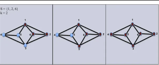
Fig. 1 Threshold functionfkfork=2. On the left, we see the original graph with only the given set S= {1,2,6}excited,fk(S)in the middle, andfk2(S)in the right
The resulting active set of nodes ofS⊆V at a thresholdkis obtained whenSis given as an input to the threshold functionfk. That is, given a subsetSof activated nodes, other nodes in the graph will become activated if they satisfy the threshold inequality, for simplicity we denotefki(S)=fk(fki−1(S))for i≥2 and fk1=fk. Figure1illustrates this process fork=2.
Definition 2 A subset of verticesSis called invariant iffk(S)=S.
Definition 3 The closure ofS, denoted clk(S), is the invariant set generated when fkn(S)=fkn−1(S)for somen≥1.
In Fig.1, the closure of the setS= {1,2,6}is achieved whenn=3, and it is the entire vertex setV.
Definition 4 A subsetS is called persistent if fk(S)⊇S, and it is called minimal persistent if no proper subset of it is persistent.
In Fig.1, the setS= {1,2,3,6}is persistent whenk=2. However,S= {1,2,6} is a persistent subset ofS, which impliesSis not minimal.
Definition 5 A subsetSis called weak if there exists ann≥1 such thatfkn(S)= ∅.
In Fig.1, the setS= {1,2}is weak, sincefk(S)= {6}andfk2(S)= ∅.
Definition 6 A tight set is a persistent setP in which every persistent subset ofP whose complement inP is not weak and excites the whole ofP.
Finally, the reader has the necessary background concepts to understand Palm’s mathematical definition of a cell assembly.
The mathematical definition of a cell assembly encompasses a variety of tight sets. For instance, in Fig.1,S is a tight set and any superset ofSis also a tight set. Yet, Palm proposed that a minimal persistent set is a tight set [19]. Therefore, we focus on the study of cell assemblies generated by minimal persistent sets.
2.2 k-Assembly
Seidman introducedk-cores to study network structure, and demonstrate thatk-core cohesion increases askincreases [23]. He defined ak-core as a maximal connected induced subgraph with degree greater than or equal tok. The maximal property of Seidman’s definition will not be considered for the topic presented in this paper. In other words, we define ak-core to only be a subgraph with minimum degree at leastk.
Definition 8 A subgraphK⊆Gis ak-core if|N (v)∩V (K)| ≥k∀v∈V (K).
Definition 9 Ak-core is minimal if no proper subset of its vertices induces ak-core.
It is clear by the definition that the subgraph generated byfk(V ), for some˜ V˜ ⊆V
is ak-core if and only if V˜ is a persistent set. That is, if fk(V )˜ is ak-core, then
for all v˜∈ ˜V|N (v)˜ ∩fk(V )˜ | ≥k, which implies V˜ ⊆fk(V ). Likewise, if˜ V˜ is a persistent set, thenV˜⊆fk(V ), which implies˜ fk(V )˜ is ak-core. In addition, note that for an unweighted graph, the threshold function definition of a tight setS becomes
fk(S)= {v∈V | |N (v)∩S| ≥k}, that is cl(S)generates ak-core. By definition, a
k-core is tight as long as its complement is not weak, since every subset of its vertex set is persistent. Hence, the closure of anyk-core generates a cell assembly.
The definition of a cell assembly tells us that it only takes a fraction of the assem-bly to get excited in order to excite the entire assemassem-bly. However, the motivation and focus of our work comes from the study of cell assemblies generated by tight sets that are minimal, that is, the deletion of any node from the set generates a subset that is not tight. In addition, the mathematical definition of a cell assembly for its study on simple graphs follows the definition of ak-core. According to Palm’s definition of a tight set, a particular type of tight set is a minimalk-core. Hence, the vertex set of a minimalk-core generates a particular type of cell assembly calledk-assembly.
Definition 10 Ak-assembly is the closure of a minimalk-core.
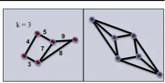
Recall this definition only holds for cases in which theGhasc(u, v)=1 for all
e=uv∈E. In Fig.2, we observe on the left that any two adjacent vertices satisfy
the definition of a cell assembly fork=3, since the edges have weights with value greater than one. Nevertheless, a set with less thank+1 vertices cannot be a minimal
k-core, and its closure is not ak-assembly. In contrast, the graph on the right has every
Fig. 2 Cell assembly vs.
k-assembly fork=3. The graph
on the left satisfies the definition
of a cell assembly, but not of
k-assembly. The graph on the
right is a 3-assembly with
c(u, v)=1 for alle=uv∈E
finding all minimalk-cores for a given simple undirected graph. Nevertheless,
find-ingk-cores is not an easy task, and we briefly discuss some complexity properties of
problems that deal withk-cores in the rest of this section.
Theorem 1 Thek-core containment problem is NP-complete.
Proof of Theorem1 The decision version of the problem is the following: Instance: Given a graphGand integerss≤ |V|.
Question: DoesGhave ak-core of sizes?
Clearly, thek-core problem belongs to NP since given a solution of the problem, a nondeterministic Turing Machine checks if the choice is true in polynomial time. Furthermore, If we restrict thek-core problem by considering only instances in which the cardinality of thek-cores=k+1, then we get the clique problem [24]. Hence,
thek-core containment problem is NP-complete.
The problem of finding all minimalk-cores also requires graphical enumeration which refers to the art of counting the number of graphs with a specific property. Note that for some problems to count the number of graphs with a given property is harder than to determine if there exists a graph that satisfies such a property. For instance, “Given a graphGand a fixed valuek >0, how many distinctk-cores are there forG?” is not a trivial problem and it empirically depends on the density of the graph. Enumeration problems associated with NP-complete problems are NP-hard [24]. This is true since the enumeration version of the problem must be at least as hard as the decision version of the problem. Hence the enumeration ofk-cores is NP-hard.
To study in depth enumeration problems the class #P was introduced [25].
Definition 11 The class #P contains all problems computed by nondeterministic polynomial time Turing machines that have the additional facility of outputting the number of accepting computations.
Moreover, #P-complete is the analog definition of NP-complete forP. The class #P asks for the number of solutions rather than their existence. For NP-complete problems counting the number of solutions is #P-complete. Therefore enumeration
ofk-cores belongs to the class of #P-complete problems.
detection [26]. However, instead of restricting it to the study of motifs of certain size, it focuses on the study of subgraphs that pass a certain threshold.
3 Previous Work on Solving the Minimal
k
-Core Enumeration Problem
The fact that a clique with vertex set cardinalityk+1 is a minimalk-core allows us to say that algorithms performing clique enumeration were the first ones to attack a subset of the problem we present in this paper.
The Maximal Clique Enumeration Problem (MCEP) asks to compile a list of all maximal cliques in a given undirected graphG. Besides its applications in sociolog-ical problems, it is also useful in the study of biologsociolog-ical networks [27]. MCEP in the worst case scenario runs exponential with respect to the number of vertices. More specifically, the maximum number of maximal cliques in an n vertex graph is 3n3 [28]. In other words, it has been proved that there may be a graph with an exponential number of maximal cliques, which implies that any algorithm that solves MCEP for an arbitrary given graph would be exponential.
Bron and Kerbosch (B&K) developed a backtracking algorithm to solve MCEP in 1973 [29]. Although other algorithms to solve the problem were developed around the same period [30], the B&K approach is still one of the most widely known to solve this problem and it is used as a basis for other algorithms that solve MCEP. For further discussion of modifications of B&K, see [31]. The B&K algorithm depends on the number of nodes in the graph, and numerical experiments show it runs inO(3.14n3) on Moon–Mooser graphs with a theoretical limit of 3n3. The B&K Algorithm will be discussed in more detail in the following section.
As MCEP, the Minimalk-core Enumeration Problem (MKEP) asks to create a list of all minimalk-cores in a given undirected graph. There is not a known bound for the maximum number of minimalk-cores on a given graph. However, the fact that a clique with vertex set cardinalityk+1 is a minimalk-core, intuitively tells us that the number of minimalk-cores grows exponentially in the worst case scenario.
A solution to MKEP through exhaustive search has been proposed, it follows the structure of a branching algorithm [32]. Their algorithm, as well as the one we pro-pose in our methods section initially obtain the maximumk-core. The following greedy algorithm obtains the maximumk-core in polynomial time [13]:
Algorithm 1 (Maximumk-core)
MaximumKcore(G)
ifGis empty
0. End
else
1. Choose a vertexv of minimum degreeδ(v)
ifδ(v)≥k
ifδ(v) < k
4. MaximumKcore(G:=G\v)
A description of the algorithm proposed by [32] is the following:
Algorithm 2 (k-Core enumeration ofG)
Given an undirected graphG=(V , E) 0. ifGis a minimalk-core
End else
1. Find the maximumk-core, call itH
for eachv∈V (H )
2. V (G):=V (H )\v
3. Go to step 1
The algorithm described above finds all minimalk-cores of a given graph. How-ever, a major disadvantage is the fact that it may return the same minimalk-core multiple times. It initially checks if the given graphGis a minimalk-core, and stops in the case it is in fact a minimalk-core. Otherwise, it proceeds to find the
maxi-mumk-core, and then minimalk-cores. No numerical results are given for thek-core
enumeration approach performance. Yet, it is mentioned that it takes minutes to enu-merate thek-cores of a graph with a vertex set of 10 nodes. The algorithm we devel-oped to solve MKEP will be discussed in our methods section and its performance is analyzed in the numerical results section.
4 Methods: Backtracking Algorithm Techniques
Backtracking is a type of recursive strategy commonly used to find all the solutions of some problem. It incrementally builds a tree in a such a way that it faces a number of options at each level, and tries all of them. In a problem withN possible solu-tions, exhaustive search techniques evaluate all the options inN trials. In contrast, a backtracking algorithm yields the solution with less thanN trials, and its solution space is organized as a tree. Initially, it starts at the root of the tree and proceeds to make a choice between one of its children, then it continues to make a choice among the children of each node until it reaches a leaf. Each leaf is either a solution of the problem or does not lead to a solution, and at that point the algorithm backtracks. For more details on backtracking algorithms, see [33] and [34].
4.1 The Bron and Kerbosch Algorithm for Finding All Cliques of an Undirected Graph
The B&K algorithm utilizes a recursively defined extension operator that is applied to three sets: compsub, not, and candidates. The set compsub contains the nodes already defined as part of the clique and it is initially empty. The set candidates is the set of nodes adjacent to all nodes in the set compsub. The set not stores the nodes that had already been processed, leading to a valid extension of the set compsub and should remain ignored. In addition to these three sets, there are nodes that are not considered at each step.
In order to obtain all maximal cliques, a backtrack search tree is constructed through recursive calls to the extension operator. Every time the recursion is called the three main sets are modified. The sets not and candidates are given to the exten-sion operator as input parameters and are locally defined. In contrast, the set compsub is globally defined and behaves like a stack. It is important to point out that if at some point the set not contains a vertex that is adjacent to all vertices in compsub, then the algorithm backtracks since no further selection of candidates will lead to obtain-ing a maximal clique from the current configuration of the set compsub. The basic mechanism can be described in the following pseudocode:
Algorithm 3 (Bron and Kerbosch)
Extension(compsub,candidates,not)
if candidates= ∅and not= ∅
1. Report compsub as a maximal clique
else For each vertexv∈candidates:
2. Select a candidates 3. Addsto compsub such that
new compsub:=compsub∪s 4. Create new sets candidates and not
by removing all points not connected tosand store old sets, that is, candidates:=candidates∩N (s)
not:=not∪N (s)
5. Extension(compsub,candidates,not) 6. Upon return, removesfrom compsub
and add it to not compsub:=compsub\s not:=not∪s
End
connected to all elements in the set candidates. If the second condition for termination is met, then the addition of any candidate to compsub will not be maximal.
To optimize the algorithm and make it terminate as early as possible, the number of times the extension operator is called must be minimized. To do this, every node in not is assigned a counter that indicates to how many candidates a node is not adjacent (or disconnected). We then proceed to pick the node with the smallest number of disconnections and on each step select a candidate not adjacent to this node.
4.2 Algorithm for Finding All Minimalk-Cores of an Undirected Graph
The problem of finding all minimalk-cores of a given graph is computationally ex-pensive. There exists a variety of algorithms to find all cliques in a given undirected graph. However, the B&K algorithm is commonly used to find all maximal cliques, since numerical experiments support its efficiency. We propose a modification of the B&K algorithm to find all minimalk-cores on a given graph.
As in B&K, the algorithm presents a backtracking technique to find all minimal k-cores. Three sets are utilized to obtain all minimalk-cores recursively, namely kcore, not, and candidates. However, since ak-core is a generalization of a clique, and every clique onk+1 or more nodes contains a minimal k-core, but not every minimal k-core is a clique, there are some subtle changes in the definition of our sets. For example, we take into account that, given a connected simple undirected graph, all minimalk-cores must be contained in the maximumk-core, which can be found in polynomial time (for more details see [13]).
The set kcore stores the nodes that are part of ak-core and is initially the entire vertex set. The set candidates contains the nodes that can be deleted to obtain a
min-imalk-core. The set not represents the nodes that had already been processed and
cannot be deleted from kcore. As in B&K, these three sets are modified by a recur-sively defined extension operator. The set kcore is globally defined, whereas the sets not and candidates are locally defined and handed as parameters to the extension operator.
We construct our backtracking search tree by recursively calling the extension operator. At the root of the search tree, the number of branches generated is equal to the cardinality of the set candidates. Each branch corresponds to removing one vertex from our configuration of the set kcore, and creating new sets candidates and not. The algorithm always selects the vertex of smallest degree one at a time. It continues traversing the search tree on a depth first search approach if there is at least one vertex in the set candidates whose deletion leads to obtaining ak-core of smaller cardinality and backtracks if the configuration of kcore cannot lead to returning a minimal k-core. That is, if the set not contains vertices that must be deleted in order to obtain a minimalk-core then no further calls to the extension operator will lead to a valid configuration of the set kcore. Hence, such a branch must not be extended. The basic idea behind the algorithm is the following:
Algorithm 4
if candidates= ∅and kcore\vi does not induce ak-core∀vi∈not
1. Report kcore as a minimalk-core
else For each vertexv∈candidates:
2. Select a candidatesof smallest degree 3. Removesfrom kcore such that
kcore:=kcore\sand candidates:=candidates\s 4. Create new sets candidates and not
and store old sets, that is,
candidates:=set of all candidates v∈V\not that still leave ak-core 5. Extension(kcore,not,candidates) 6. not:=not∪s
kcore:=kcore∪s
candidates:=candidates\s
The majority of the steps described above are straightforward to implement. How-ever, there are several different options on how to implement step 2, which is how to select a well-chosen candidate to minimize the number of times the extension opera-tor is called. At the moment, it is impossible to give a good theoretical explanation on why one way to choose a candidate is better than another. They vary on a case by case basis, and its efficiency is determined by observations on numerical experiments. We chose to select a candidate of minimum degree because this way ensures that the set not is filled in correctly. However, modifying the original given set of candidates to be in the form required to be a candidate and selecting the candidate of maximum de-gree will also yield a solution to our problem. Figure3displays the backtrack search tree of our algorithm for a given graphG.
Now, we have to show that our proposed algorithm terminates and performs cor-rectly. Clearly, for a given graph Gwith finite vertex and edge sets the algorithm terminates since the number of subgraphs to enumerate is finite. However, the num-ber of subgraphs in a given graphGdepends on its structure, and it may be very large for dense graphs. The next theorem is of extreme importance in showing correctness of Algorithm4, since it guarantees that for every subgraph that contains ak-core all its minimalk-cores are generated without duplication.
Theorem 2 The extension of the backtracking search tree for a given configuration
of the set kcore by applying the extension operator generates all minimalk-cores without repetition that contain kcore\vi ∀vi∈candidates
Proof of Theorem2 This proof is by strong induction on the cardinality of the set kcore.
Fig
.
3
Backtrack
search
tree
for
a
gi
v
en
g
raph
G
.
T
he
root
of
the
tree
contains
the
entire
g
raph
and
the
lea
v
es
contain
m
inimal
k
-cores
or
ex
tensions
that
made
the
algorithm
backtrack.
T
he
sets
kcor
e,
not
,a
n
d
candidates
follo
w
the
definitions
of
Algorithm
deletion of this vertex contains ak-core. The case|candidates|>0 is not possible, since it implies that there exists ak-core of cardinality less than or equal tok, which is false by the definition of ak-core.
Now suppose that the statement is true for alll > k∈Z such that l ≤N, and that all minimalk-cores obtained by removing an element of not from the current configuration of the set kcore have been previously generated. We can suppose the later since it is guaranteed by our definition of the set candidates.
Consider a configuration of kcore with cardinalityN+1. Let{v1, . . . , vc}
repre-sent the set of candidates forc≥0. If|candidates\vi| =0 for some 0≤i≤cthen we see that kcore is a minimalk-core.
If|candidates\vi|>0, then we have the following two cases:
Choosev˜ as in step 2 of our algorithm and create a new set of candidates:= candidates\ ˜v, proceed to call extension(kcore\ ˜v,candidates,not). If the cardinality of the new set of candidates is greater than 0, then by the inductive hypothesis the statement is true forl=N+1. If it is zero then kcore\ ˜vis not minimal, andv˜ is added to not. Which completes our proof and we see that Theorem2is true∀n∈Z.
Since Theorem2is true for any subgraph of any given finite cardinality, we see that Algorithm4finds all minimalk-cores of a given undirected graph without rep-etition. In the following section, the results from running the backtracking algorithm for several test instances are presented.
5 Numerical Results
Algorithm 4 was implemented using C++ and tested in workstation with a AMD Opteron(tm) Processor 148. Results of numerical experiments are run to test the backtracking algorithm on random graphs. More specifically, we utilized graphs that follow a Bernoulli process in the generation of edges and are known as Bernoulli ran-dom graphs, as well as regular graphs. The existence of an edge in Bernoulli ranran-dom graphs occur independently between each pair of nodes. For instance, given some probabilitypand the number of verticesn, there exists an edge(i, j ), wherei=j and 0< i, j ≤n. In contrast, regular graphs have the property that each vertex has the same degree.
A summary of the obtained results is presented at the end of this section, where 100 Bernoulli random graphs were generated for each test instance, then the average time and number ofk-cores were computed among the number of graphs that in fact contained at least onek-core fork=2,3 and 5.
The average number of minimalk-cores is displayed to highlight the fact that the number of minimalk-cores depends on the density of the graph, and not on the value
ofk. Even though everyk-core is ak−1-core, the fact that we restrict our solution
set tok-cores that are minimal give us cases in which the number ofk-cores is greater that the number ofk−1-cores.
Table 1 Algorithm4
performance forn=10 and
p=0.1,0.5 and 0.7
k p # ofk-cores Average time # of graphs
2 0.1 1.1764 ≈0 s 17
3 0.1 0 ≈0 s 0
5 0.1 0 ≈0 s 0
2 0.5 27.72 ≈0 s 100
3 0.5 12.2041 ≈0 s 98
5 0.5 1 ≈0 s 6
2 0.7 57.14 0.0001 s 100
3 0.7 54.02 ≈0 s 100
5 0.7 5.4634 ≈0 s 82
Table 2 Algorithm4
performance forn=15 and
p=0.1, 0.5 and 0.7
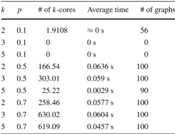
k p # ofk-cores Average time # of graphs
2 0.1 1.9108 ≈0 s 56
3 0.1 0 0 s 0
5 0.1 0 0 s 0
2 0.5 166.54 0.0636 s 100 3 0.5 303.01 0.059 s 100 5 0.5 25.22 0.0029 s 90 2 0.7 258.46 0.0577 s 100 3 0.7 630.02 0.0604 s 100 5 0.7 619.09 0.0457 s 100
and 0.7 and the value ofk=2,3 and 5. # ofk-cores denotes the average number of k-cores on the tested graphs, and # of graphs is the number of graphs that at least contained onek-core.
In Table1, we observed the results for graphs with 10 vertices. The graphs gener-ated with probability 0.1 only had a few 2-cores, since they are not dense enough to even containk-cores for larger values ofk. As the probability increased, we observed that more minimal 3-cores and 5-cores were part of the random graphs. However, the average number of minimal 2-cores is always greater than 3-cores and 5-cores. It is important to point out that we observe this behavior only because the vertex set cardinality is small. But it is not always the case that we have more minimal 2-cores than minimal 3-cores as we will see in the later results.
In Table2, the results for graphs with 15 vertices are displayed. We still observe a low existence of minimalk-cores for sparse graphs withp=0.1. However, graphs generated with probabilities 0.5 and 0.7 show a different behavior and contain a larger number ofk-cores. Note that in contrast to graphs on 10 vertices, on these cases the number of minimal 3-cores is larger than the number of minimal 2-cores and decreases again for the number of 5-cores.
Table 3 Algorithm4
performance forn=20 and
p=0.1,0.5 and 0.7
k p # ofk-cores Average time # of graphs 2 0.1 6.8370 1.8583 s 92
3 0.1 2 0.485 s 2
5 0.1 0 0 s 0
2 0.5 635.11 2.3256 s 100 3 0.5 3511.19 1.4819 s 100 5 0.5 2661.11 0.0029 s 100 2 0.7 791.66 2.0905 s 100 3 0.7 3902.45 2.3057 s 100 5 0.7 17010.33 2.9131 s 100
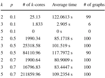
Table 4 Algorithm4
performance forn=25 and
p=0.1, 0.5 and 0.7
k p # ofk-cores Average time # of graphs 2 0.1 25.13 122.0613 s 99 3 0.1 1.833 2.905 s 6
5 0.1 0 0 s 0
2 0.5 1990.34 85.1718 s 100 3 0.5 25318.58 101.519 s 100 5 0.5 84110.96 117.7972 s 90 2 0.7 1900.64 80.9009 s 100 3 0.7 16796.83 83.4447 s 100 5 0.7 211859.96 109.2354 s 100
is observed in Table4for random graphs on 25 vertices with p=0.5 and 0.7. In terms ofk-assemblies, we observe that at a fixed threshold the number of minimal sets that generate ak-assembly increase askincreases. This tells us that the number of minimal 2-cores is smaller than the number of minimal 3-cores and 5-cores, which is not true in general if thek-cores are not minimal.
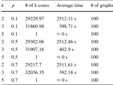
In Table 4, we observe an interesting phenomenon, which is that Algorithm 4 finds all minimalk-cores of a random graph faster when the graph is dense for the three values ofk utilized to test it. Although this result may seem counterintuitive, observations showed that the algorithm backtracks faster whenever it is dealing with a dense graph. Algorithm4initially takes longer to output the first minimalk-core for a dense graph than for a sparse one. However, after the first minimalk-core is found; it backtracks to deal with more cases in which minimalk-cores in fact exist and with less configurations of the set compsub that do not lead to obtaining a minimalk-core. In addition to Bernoulli random graphs, random 5-regular graphs with n=30 were tested to check if we observe the same behavior as in random graphs, see Ta-ble5. As expected they only had one minimal 5-core. However, they also contain a greater number of 3-cores than 2-cores.
Nonethe-Table 5 Algorithm4
performance for 5-regular graphs withn=30 and
p=0.1,0.5 and 0.7
k p # ofk-cores Average time # of graphs 2 0.1 29229.97 2512.11 s 100 3 0.1 31860.98 398.71 s 100
5 0.1 1 ≈0 s 100
2 0.5 29302.06 2512.46 s 100 3 0.5 31907.16 402.9 s 100
5 0.5 1 ≈0 s 100
2 0.7 29217.7 2511.61 s 100 3 0.7 32036.35 392.18 s 100
5 0.7 1 ≈0 s 100
less, it is still necessary to check if these types of graphs follow the same behavior as Bernoulli random graphs, since the brain is neither completely random nor regular.
6 Discussion
In this paper, we proposed a backtracking algorithm to find all minimalk-cores whose excitation can activate ak-assembly. The motivation to study this problem emerges from the urge to understand memory. Palm formulated the main problem of the theory of cell assemblies by asking the total number of cell assemblies at a given thresholdk. The proposed algorithm is closely related to this problem since it allows us to find the total number of subsets that generatek-assemblies on a given graph. Through numerical experiments we confirm that fractions of these important subsets overlap. These overlappings tell us that concepts are organized in groups and certain triggers activate associated memories.
An extension to the graph theoretical approach for the analysis of associative memory introduced by Palm is presented along with details on the derivation of the
k-assembly from the cell assembly model. Although Algorithm4is not fast enough
to solve the problem in a brain-sized neuronal network, it does offer a solution to the problem, permits us to analyze the structure of a given random graph and gain insight on understandingk-assemblies and cell assemblies. For instance, the fact that for some graphs there may be a larger number of minimal 5-cores than 3-cores al-lowed us to observe how the structures overlap. If we look at it in terms of memory, we can tell that certain nodes are members of severalk-assemblies, and the absence of one of them may change the structure of the network completely. If larger data sets become available we could use standard techniques for network clustering ork-core decomposition that would allows us to partition the graph and find minimalk-cores within the partitions.
of thek-cores obtained from the undirected graph is still ak-core in terms of in or out degree.
The objective of this project was to gain understanding about the k-assembly model and to solve the problem of finding all minimalk-cores of an undirected graph. There is still much to explore in the model of thek-assembly. In particular, it would be interesting to study thek-assembly for a non-fixed value ofk. For this approach, it would be necessary to analyze the change in the value ofk with respect to time and design a dynamical system on the graph. In terms of the algorithm, a promising research direction is to explore the structure of the graph to minimize the number of times the extension operator is called; this would be extremely helpful for solving the problem on sparse graphs. In general, the problem of finding all minimalk-cores continues to be difficult to solve due to the fact the number of minimalk-cores in a graph grows with the number of vertices and edges. Therefore, any condition that makes Algorithm4backtrack faster or that minimizes the number of times the ex-tension operator is called would be a significant contribution to the solution of the problem.
Competing Interests
The authors declare that they have no competing interests.
Authors’ Contributions
CW contributed in the design and implementation of the algorithm, generation of data and prepared this manuscript. IH contributed in the design and implementation of the algorithm, carefully reviewed and improved the contents of this manuscript.
Acknowledgements This work is made possible by the National Science Foundation Grants Number 0940902 and CMMI-1300477.
References
1. Wasserman S, Faust K. Social network analysis methods and applications. Cambridge: Cambridge University Press; 1994.
2. Borgatti SP, Mehra A, Brass DJ, Labianca G. Network analysis in the social sciences. Science. 2009;323(5916):892–5. doi:10.1126/science.1165821.
3. Proulx SR, Promislow DEL, Phillips PC. Network thinking in ecology and evolution. Trends Ecol Evol. 2005;20(6):345–53. doi:10.1016/j.tree.2005.04.004.
4. Rubinov M, Sporns O. Complex network measures of brain connectivity: uses and interpretations. NeuroImage. 2010;52(3):1059–69. doi:10.1016/j.neuroimage.2009.10.003.
5. Sporns O. Networks of the brain. Cambridge: MIT Press; 2011. 6. Hebb DO. The organization of behavior. New York: Wiley; 1949.
7. Luce RD, Perry AD. A method of matrix analysis of group structure. Psychometrika. 1949;14(2):95– 116.
8. Festinger L. The analysis of sociograms using matrix algebra. Hum Relat. 1949;2(2):153–8. 9. Miller DA, Zucker SW. Computing with self-excitatory cliques: a model and an application to
10. O¸san R, Chen G, Feng R, Tsien JZ. Differential consolidation and pattern reverberations within episodic cell assemblies in the mouse hippocampus. PLoS ONE. 2011;6(2):16507. doi:10.1371/journal.pone.0016507.
11. Lin L, Osan R, Shoham S, Jin W, Zuo W, Tsien JZ. Identification of network-level coding units for real-time representation of episodic experiences in the hippocampus. Proc Natl Acad Sci USA. 2005;102(17):6125–30. doi:10.1073/pnas.0408233102.
12. Seidman SB, Foster BL. A graph theoretic generalization of the clique concept. J Math Sociol. 1978;6:139–54.
13. Balasundaram B, Butenko S, Hicks IV, Sachdeva S. Clique relaxations in social network analysis: the maximumk-plex problem. Oper Res. 2011;59(1):133–42.
14. Thai MT, Pardalos PM, editors. Handbook of optimization in complex networks: communication and social networks. Berlin: Springer; 2012.
15. Palm G. On associative memory. Biol Cybern. 1980;36:19–32.
16. Collins AM, Loftus EF. A spreading-activation theory of semantic processing. Psychol Rev. 1975;82(6):407–28.
17. Curto C, Itskov V. Cell groups reveal structure of stimulus space. PLoS Comput Biol. 2008;4(10):1000205. doi:10.1371/journal.pcbi.1000205.
18. Tsukada M, Ichinose N, Aihara K, Ito H, Fujii H. Dynamical cell assembly hypothesis—theoretical possibility of spatio-temporal coding in the cortex. Neural Netw. 1996;9(8):1303–50.
19. Palm G. Towards a theory of cell assemblies. Biol Cybern. 1981;39:181–94.
20. Braitenberg V. Cell assemblies in the cerebral cortex. In: Theoretical approaches to complex systems. Berlin: Springer; 1978. p. 171–88.
21. Palm G, Knoblauch A, Hauser F, Schüz A. Cell assemblies in the cerebral cortex. Biol Cybern. 2014;108(5):559–72.
22. Picado-Muiño D, Borgelt C, Berger D, Gerstein G, Grün S. Finding neural assemblies with frequent item set mining. Front Neuroinform. 2013;7: 9.
23. Seidman SB. Network structure and minimum degree. Soc Netw. 1983;5:269–87.
24. Garey MR, Johnson DS. Computers and intractability: a guide to the theory of NP-completeness. New York: W.H. Freeman and Company; 1979.
25. Valiant LG. The complexity of computing the permanent. Theor Comput Sci. 1979;8:189–201. 26. Sporns O, Kötter R. Motifs in brain networks. PLoS Biol. 2004;2(11):369.
27. Bron C, Kerbosch J, Schell HJ. Finding cliques in an undirected graph. Technological University of Eindhoven; 1972 Feb. Technical report.
28. Moon J, Mooser L. On cliques in graphs. Isr J Math. 1965;3(1):23–8.
29. Bron C, Kerbosch J. Finding all cliques of an undirected graph. Commun ACM. 1973;16:575–7. 30. Akkoyunlu EA. The enumeration of maximal cliques of large graphs. SIAM J Comput.
1973;2(1):1–6.
31. Cazals F, Karande C. A note on the problem of reporting maximal cliques. Theor Comput Sci. 2008;407(1–3):564–8.
32. Cox SJ, Cavazos J, Halani K, Rubenstein Z. Cell assembly enumeration in random graphs. Rice University; 2010. Technical report.
33. Knuth DE. The art of computing programming. vol. 2. Reading: Addison-Wesley; 1968. p. 198–213. 34. Leiserson CE, Rivest RL, Stein C, Cormen TH. Introduction to algorithms. Cambridge: MIT Press;