R E S E A R C H
Open Access
Real-time obstacle avoidance of mobile
robots using state-dependent Riccati
equation approach
Seyyed Mohammad Hosseini Rostami
1, Arun Kumar Sangaiah
2, Jin Wang
3and Hye-jin Kim
4*Abstract
In this paper, state-dependent Riccati equation (SDRE) method-based optimal control technique is applied to a robot. In recent years, issues associated with the robotics have become one of the developing fields of research. Accordingly, intelligent robots have been embraced greatly; however, control and navigation of those robots are not easy tasks as collision avoidance of stationary obstacles to doing a safe routing has to be taken care of. A moving robot in a certain time has to reach the specified goals. The robot in each time step needs to identify criteria such as velocity, safety, environment, and distance in respect to defined goals and then calculate the proper control strategy. Moreover, getting information associated with the environment to avoid obstacles, do the optimal routing, and identify the environment is necessary. The robot must intelligently perceive and act using adequate algorithms to manage required control and navigation issues. In this paper, smart navigation of a mobile robot in an environment with certain stationary obstacles (known to the robot) and optimal routing through Riccati equation depending on SDRE is considered. This approach enables the robot to do the optimal path planning in static environments. In the end, the answer SDRE controller with the answer linear quadratic controller will be compared. The results show that the proposed SDRE strategy leads to an efficient control law by which the robot avoids obstacles and moves from an arbitrary initial point × 0 to a target point. The robust performance of SDRE method for a robot to avoid obstacles and reach the target is demonstrated via simulations and experiments. Simulations are done using MATLAB software.
Keywords:Optimal control, Nonlinear control, Obstacle avoidance, SDRE
1 Introduction
A mobile intelligent robot is a useful tool which can lead to the target and at the same time avoid an obstacle when faced with it. Obstacle avoidance means that the robot avoids colliding with obstacles such as fixed objects or moving objects. So when a robot encounters with an obstacle, it must decide to avoid it and at the same time, consider the most efficient path to the target with a good decision; this decision is performed in this research using the state-dependent Riccati equation (SDRE) control method. The optimal control of nonlin-ear systems cannot be done similar to the methods of linear systems. One of the significant viewpoints for
optimal control of nonlinear systems is using the SDRE. This method in addition to stability creates a proper functioning and robust for a wide range of nonlinear systems. Nonlinear optimal controller SDRE is a devel-oped linear optimal control LQR, in which equations Riccati is state-dependent. Strategy SDRE has been introduced in the past decade. This strategy is a very effective algorithm for feedback nonlinear analysis that its states are nonlinear; however, a flexibility idea of through the weight matrix is dependent on the state. This involves factoring (ie, parameterization) of nonlin-ear dynamics to state vector and produces a value func-tion for the matrix which is dependent on its state.
There are conventional methods of obstacle avoid-ance such as the path planning method [1], the navi-gation function method [2], and the optimal regulator [3]. Hence, an SDRE regulator [4, 5] is used for this
* Correspondence:[email protected]
4Business Administration Research Institute, Sungshin Women’s University, Seoul, Republic of Korea
Full list of author information is available at the end of the article
paper. In recent years, many researchers have investi-gated the obstacle avoidance problem from different perspectives. SDRE technique developed as a design method, which provides a systematic and effective de-sign of nonlinear controllers, filters, and observers. Be-cause of its versatile features, SDRE is broadly used for different cases [6–14]. SDRE can also be used in the field of medicine, for example, in [15,16] the presenta-tion of the optimal chemotherapy protocol for cancer treatment, considering the metastasis, has used the full optimal SDRE feedback. In [17], the SDRE algorithm is studied on motion design of the cable-suspended robot with uncertainties and moving obstacles. A method for controlling the tracing of a robot has been developed by the SDRE. Vibration control of flexible-link manipu-lator in [18] is used in SDRE controller and Kalman fil-tering. The problem of estimating flexural states during the use of the SDRE for flexible control is the focus of this paper. Wanga et al. [19] present a novel H2−
H∞SDRE control approach with the purpose of provid-ing a more effective control design framework for continuous-time nonlinear systems to achieve a mixed nonlinear quadratic regulator and H∞control perform-ance criteria.
It should be noted that the algorithms discussed for avoiding an obstacle are different from each other, and each algorithm has proposed a separate and new method for avoiding obstacles. So far, novel methods to avoid obstacles in addition to the mentioned methods are also presented [20–23].
This paper is organized as follows: a description of the SDRE formulation is given in Section 2. Then, motion equations of the robot and its constraints are presented in Section 3. In Section 4, SDRE formulation of the robot is derived. And simulation results have been re-ported in Section 5. Finally, in Section 6, some conclu-sions are drawn from this research.
2 Methods
2.1 Problem formulation
Consider a nonlinear system that is autonomous, full-state observable and input affine that is presented as follows:
_
x tð Þ ¼f xð Þ þB xð Þu tð Þ;xð Þ ¼0 x0 ð1Þ
Where x∈Rn is the state vector, u∈Rm is the input vector, and t∈[0,∞), with functions f:Rn→Rnand B:
Rn→Rn×m, andB(x)≠0∀x. Without any loss of gener-ality, the origin is assumed to be an equilibrium point, such that f(0) = 0. In this context, the minimization of the infinite-time performance criterion is as follows:
J xð 0;uð Þ:Þ ¼ 1 2
Z
xTð Þt Q xð Þx tð Þ þuTð Þt R xð Þu tð Þ
dt
ð2Þ
Consider the above equation which is non-quadratic in x but quadratic in u. The state and input weighting matrices are assumed state-dependent such that Q:
Rn→Rn×nand R:Rn→Rn×m. These design parameters satisfyQ(x)≥0 andR(x) > 0 for allx[24].
2.2 SDRE nonlinear regulator problem
The SDRE methodology uses extended linearization as the key design concept in formulating the nonlinear optimal control problem. The linear control synthesis method for this case is the LQR synthesis method. SDRE feedback control is an “extended linearization control method” that provides a similar approach to the nonlinear regulation problem for the input-affine system (1) with cost functional (2). The nonlinear system of (1) can be rewritten in the linear structure using SDC form:
_
x tð Þ ¼A xð Þx tð Þ þB xð Þu tð Þ ð3Þ
SDC form is not unique and should be chosen in
such a way that fQ1
2ðxÞ;AðxÞg and {A(x),B(x)} are pointwise observable and pointwise stabilizable, respectively.
Where W(x) is obtained from the solution of algebraic SDRE:
W xð ÞA xð Þ þATð ÞxW xð Þ
þQ xð Þ−W xð ÞB xð ÞR−1BTð ÞxW xð Þ
¼0 ð4Þ
to getW(x)≥0.
Where W(x) is the unique, symmetric, positive-definite solution of the algebraic state-dependent Riccati equation. As a result of this, the nonlinear control is obtained as:
u tð Þ ¼−R−1ð Þx BTð ÞxW xð Þx tð Þ ð5Þ
The response obtained is locally asymptotically stable and is optimal [25].
2.3 SDRE nonlinear tracking problem
Consider an infinite-time nonlinear tracking problem. Minimize the following nonlinear cost function that is nonquadratic inxbut is quadratic inu[26]:
J ¼1 2
Z ∞
0 E
Tð Þt Q xð ÞE tð Þ þuTð Þt R xð Þu tð Þ
dt ð6Þ
E tð Þ ¼X tð Þ−Xdesiredð Þt ð7Þ
Q,R, x, anduare like the previous model and with the same conditions. By solving the Eq. (6), the input is obtained as the following equation:
u tð Þ ¼−R−1ð Þx BTð Þx W xð ÞðX−XdÞ ð8Þ
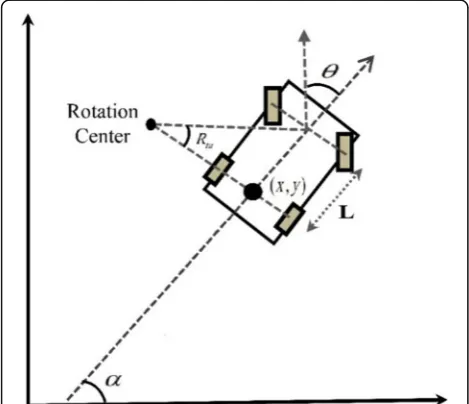
3 The four-wheeled car
Here is considered a four-wheeled robot with front-wheel drive as Fig. 1. In this robot model, Rtu instantaneous turning radius, L length between the rear axle and the front of the robot, and (x,y) the robot’s position is mea-sured at the center point of the rear wheels of the robot. The state vector consists of two-position variables (x,y), one orientation variable (θ), the speed of the robot (V), and front-wheel drive angle (α). Only the front wheels swivel in two directions, and the rear wheels swivel with-out slipping. The main reason for choosing this system for this project is the non-holonomic boundary movement of this system [27].
Here, (V) and (θ) are considered as input vectors, but using these control inputs, this system is faced with solutions that are not smooth. It is very obvi-ous that in practice mode, the speed of the vehicle’s robot and the wheel angle cannot change quickly and instantaneously. Therefore, to smooth the (V,θ) controls and make it possible to apply inputs to a real robot, a control level is added. In other words, (V,θ) is recorded as part of the state vector and (β,ψ) is added as a new control vector. These changes create smoother paths for (V,θ) that can be used in a real robot. Finally, with regard to all these
points, the equation of motion for the robot kine-matics derived as follows [27].
_ x _ y _ α _ V _ θ 2 6 6 6 6 4 3 7 7 7 7 5¼
V cosα V sinα V
L tanθ
β ψ 2 6 6 6 6 6 4 3 7 7 7 7 7 5
ð9Þ
3.1 Vehicle’s constraints
The constraints of the state and control inputs are as follows:
x∈X ¼
x:0≤x tð Þ≤10 y:0≤y tð Þ≤10
α:−3π≤α≤3π V :−30≤V≤þ30
θ:−1≤θ≤þ1
8 > > > > < > > > > : 9 > > > > = > > > > ;
u∈U¼ ψβ:−:0−:1033≤≤ψαð Þt ≤10 t
ð Þ≤0:33
ð10Þ
So far, dynamic equations of the robot and correspond-ing constraints on states and control input have been pre-sented. In the following section, the proper formulation for utilizing SDRE approach for robot motion control will be presented.
4 Implementation of SDRE controller for the robot
4.1 SDC parameterization
The first step in designing the SDRE controller is to formulate the SDC. The most important point in SDC parameterization is that factorization should provide appropriate control over the entire area. SDC presenta-tion of the system is written as follows [28].
A xð Þ ¼
0 0 β13 β14 0 0 0 β23 β24 0 0 0 0 β34 β35
0 0 0 0 0
0 0 0 0 0
2 6 6 6 6 4 3 7 7 7 7 5B xð Þ
¼ 0 0 0 0 0 0 1 0 0 1 2 6 6 6 6 4 3 7 7 7 7
5 ð11Þ
β13¼
β1Vðcosα−1Þ
α ;β14¼ð1−β1Þðcosα−1Þ þ1
β23¼β2V sincð Þα;β24¼ð1−β2Þsinα
β34¼ 1−β3
tanθ
L ;β44¼β3 V L tanθ θ
ð12Þ
4.2 Obstacle avoidance
In this paper, the concept of the APF method and the navigation function [29] is used to avoid collisions with obstacles during the robot’s movement. The navigation function that is similar to the APF, with the help of the sensor, will detect obstacles and avoid them and converge the robot toward the target. This function has the local minimum at the destination and a local maximum at the obstacles.
In the modified model, OBS can be decomposed into
obsaandobsb. Whereobsais the component force under the direction along the line between the robot and the obstacle, andobsbis the component force under the dir-ection along the line between the robot and the target.
m is a weighting factor that one can set the distance of the robot from an obstacle during movement. By setting
mand z, the desired result is achieved which is obstacle avoidance and reach the target. The proposed navigation function added to the cost function is as follows:
f
Rat¼
ffiffiffiffiffiffiffiffiffiffiffiffiffiffiffiffiffiffiffiffiffiffiffiffiffiffiffiffiffiffiffiffiffiffiffiffi
x−xd
ð Þ2þ y−yd
ð Þ2
q
Rrep¼
ffiffiffiffiffiffiffiffiffiffiffiffiffiffiffiffiffiffiffiffiffiffiffiffiffiffiffiffiffiffiffiffiffiffiffiffiffiffiffi
x−xob
ð Þ2þ y−yob
ð Þ2
q
−Rob
obsa ¼m Rat z
Rrep2þ0:1
obsb ¼ Rat z−1 ð Þ
Rrep2þ0:1
OBS¼obsaþobsb
ð13Þ
The form of obstacles is a sphere with center (xob,yob)
and radiusRob, and it is supposed that they do not
over-lap each other. The purpose of this study is to design a
control law by which the controlled object avoids obsta-cles and moves from an arbitrary initial point x0to the
destination point xd. In the next step, this obstacle avoidance equation is added to the cost function. The purpose here is to minimize the performance of the cri-terion function that is considered as follows:
J ¼1 2
Z ∞
0
ETð Þt Q xð ÞE tð Þ þuTð Þt R xð Þu tð Þ þOBS
dt
ð14Þ
Then, using the factoring, the matrix Q(x) is obtained as follows:
Q xð Þ ¼ diag 1 EX2
OBS
ð Þ; 1
EY2 OBS
ð Þ;1;1;1
fEX¼x−xd EY ¼y−yd
ð15Þ
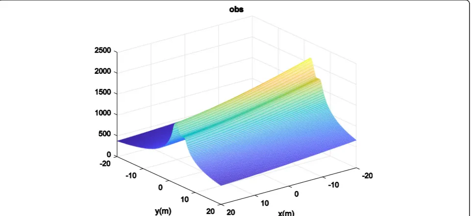
EX and EYare errors of position. Q(x) is not a single matrix and many matrices are obtained for it. By using this formulation, the robot can now start from an initial point and reach a destination while avoiding obstacles. The useful property of the obstacle avoidance term in the cost function led to the increase in the cost function while the robot is nearing obstacle and decreasing when leaving it. Figure2shows mesh plot of obstacle avoidance term in which the function has the global minimum at the destination and a local maximum at the obstacle. By rewriting (15), the second obstacle in the motion plan-ning algorithm can be constructed as follows.
Q xð Þ ¼ diag 1 EX2
OBS1þOBS2
ð Þ; 1 EY2
OBS1þOBS2
ð Þ;1;1;1
ð16Þ
5 Results and discussion
In this section, the effectiveness of the proposed method is verified by the simulation model of the robot. The general parameters include all states are as follows:
β1¼0:715;β2¼0:8;β3¼0:5
R¼ diag 1ð½ ;1Þ;L¼0:5 ð17Þ
Figure 2 shows the mesh plot of the obstacle avoid-ance term in which the function has the global mini-mum at the destination and a local maximini-mum at the obstacle. It shows that the obstacles like the summit and the target act like the cavity and absorbs the robot into the inside itself.
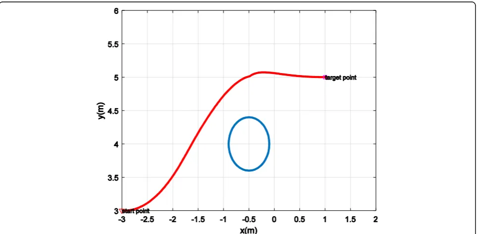
In Fig. 3, obstacles have been considered as a circle of radius 0.4 and show that with SDRE method, the robot avoids obstacles and reaches the target with minimal cost. When the robot is faced by an obstacle;
Q parameter is designed so that increases the cost function and in other words, finds the highest pos-sible value to avoid colliding with the obstacle. Here, to avoid collision with the obstacle and reach the desired target, the value of m and z in the navigation obsis respectively put 5 and 2.
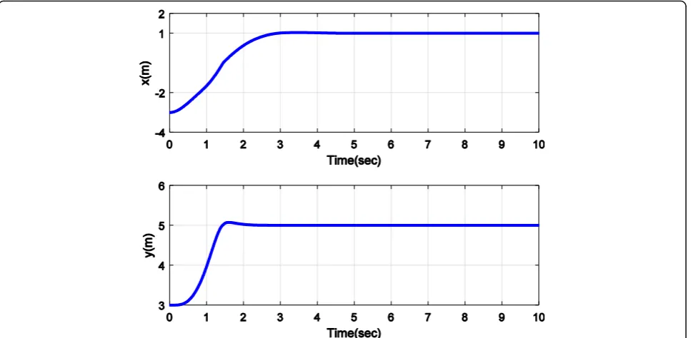
Figure 4 shows two variables x and y in reaching the target point xd= (1, 5), and these figures show that the
robot stops as soon as reaching to the target. Figure 5
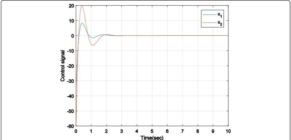
shows that other states also regulated to zero after 3.1 s. Figure 6 shows control inputs that are applied to reach the desired target, after reaching the target became zero. The purpose of this control method is to find the con-trol inputs that are applied to the system with Eq. (11); while stabilizing the system and satisfying the con-straints defined for it, the defined cost function (16) is minimized, and the system state variables converge to zero with the least control effort. The figures obtained from the simulation show that SDRE method has achieved the desired goals. By comparing this method with the modified APF method, it is observed that this method selects a more optimal route according to the definition of the cost function for avoiding the obstacle and reaching the goal. The other difference is that in SDRE method, three parameters are added: vehicle velocity (V), the angle of the front wheels (α), and length of the car between the front and rear axles (L), to design appropriate control function in order to avoidance obstacles and reach the desired target.
Without taking navigation function and supposing
Q(x) = diag[100, 100, 1, 1, 1], Fig. 7 shows that the robot cannot reach the target with obstacle avoidance. Figure8
of the LQR method in which a nonlinear system is line-arized around the vector Xv= [1, 1, 1, 1, 1]Tand initial conditionsXp= [−3,3,0.0001,0.0001,0.0001]T. Figure 9 shows that although the control inputs became zero, as Fig. 8 depicts, the robot cannot avoid obstacles in reaching to the target. Like Fig. 8, in LQR method, with linearization of around none of the operating points and
initial conditions, the robot cannot avoid obstacles in reaching to the target, so is concluded, by SDRE method where the matrix Adepends on its states, the answer is better.
In the second section, the effectiveness of the pro-posed method is verified by the simulation model of the robot. The general parameters include all states are as follows:
β1¼0:1;β2¼0:78;β3¼0:88
R¼ diag 1ð½ ;1Þ;L¼0:5 ð18Þ
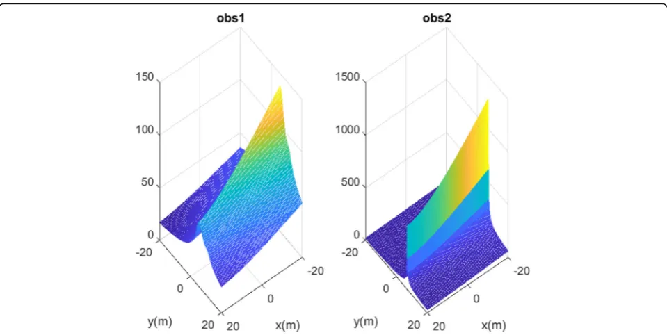
Figure 10 shows the mesh plot of the obstacle’s avoidance term in which the function has the global minimum at the destination and a local maximum at the obstacle. It shows that the obstacles like the summit and the target act like the cavity and absorbs
Fig. 5θ,Vandφtrajectories in presence obstacle point (x0,y0) = (−2, 4) and target point (xd,yd) = (1, 5) while avoiding an obstacle with SDRE method
the robot into the inside itself. Here, to avoid colli-sion with the obstacle and reach the desired target, the value of m and z in the navigation obs is respect-ively put 0.5 and 2. In the face of obstacles more than an obstacle. The principles of work for other obstacles are like one obstacle, but in this case, a
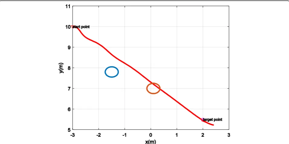
navigation function is put. For example, in Fig. 11, two obstacles have been considered as a circle of radius 0.25 and shows that with SDRE method; the robot avoids obstacles and reaches the target with minimal cost. Figure 12 shows the curve of two vari-able’s xand y in reaching the target point xd= (2, 5.5),
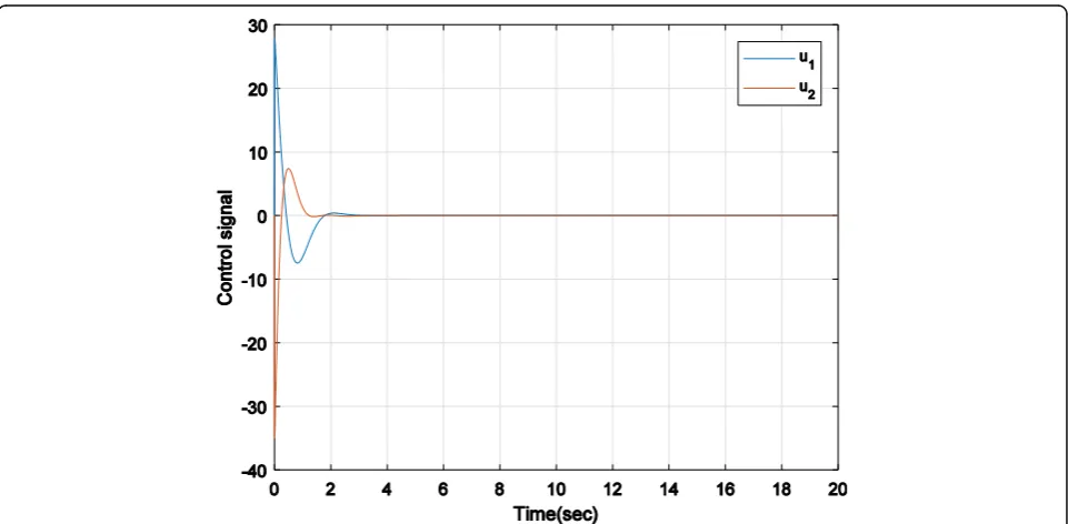
Fig. 6Control inputs applied to the robot to reach the target point (xd,yd) = (1, 5) and in presence obstacle avoidance point (x0,y0) = (−2, 4) with
SDRE method
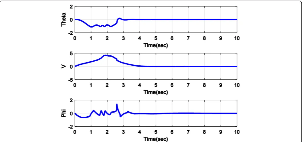
and these figures show that the robot stops as soon as reaching to the target. Figure 13 shows that other states also regulated to zero after 4.2 s. Figure 14
shows control inputs that are applied to reach the desired target, after reaching the target the control attempt becomes zero.
Without taking navigation function and supposingQ(x) = diag[100, 100, 1, 1, 1], Fig15shows that the robot cannot
reach the target with obstacle avoidance. Figure16of the LQR method in which a nonlinear system is linearized around the vector Xv= [1, 1, 1, 1, 1]Tand initial conditions
Xp= [−3,3,0.0001,0.0001,0.0001]T. Figure17shows that al-though the control inputs became zero, as Fig.16depicts, the robot cannot avoid obstacles in reaching to the target. Like Fig.16, in LQR method, with linearization of around none of the operating points and initial conditions, the
Fig. 8Path of the robot to the target point (xd,yd) = (1, 5) in presence obstacle point (x0,y0) = (−2, 4) with LQR method
robot cannot avoid obstacles in reaching to the target, so is concluded, by SDRE method where the matrix A de-pends on its states, the answer is better.
6 Conclusions
This paper focuses on the SDRE nonlinear regulator for solving the nonlinear optimal control problems.
The existence of solutions as well as optimality and stability properties associated with SDRE controllers are the main of this paper. The paper is organized as follows. In Section 2, the formulation of the nonlinear optimal control problem, the concept of extended linearization and the SDRE controller for nonlinear optimal regulation are presented, then the
Fig. 10The mesh plot of obstacle’s avoidance term in presence obstacle point’s (x01,y01) = (−1.5, 7.8), (x02,y02) = (0.1, 7) and target point (xd,yd) = (2, 5.5)
Fig. 11Path of the robot in presence obstacle points (x01,y01) = (−1.5, 7.8), (x02,y02) = (0.1, 7) and target point (xd,yd) = (2, 5.5) while avoiding
additional degrees of freedom provided by the nonuniqueness of the SDC parameterization is reviewed. The necessary and sufficient conditions on the existence of solutions to the nonlinear optimal control problem, in particular, by SDRE feedback control, are reviewed. A theoretical study on the stability and
optimality properties of SDRE feedback controls is pur-sued. SDRE method is compared with LQR method. It is concluded for that SDRE is a semilinear method, give the best answer than linear methods for nonlinear systems, because the basis of this method is that takes nonlinearity of the system and creates the nonlinear system that its
Fig. 12xandytrajectories in presence obstacle points (x01,y01) = (−1.5, 7.8), (x02,y02) = (0.1, 7) and target point (xd,yd) = (2, 5.5) while avoiding
obstacles with SDRE method
Fig. 13θ,Vandφtrajectories in presence obstacle points (x01,y01) = (−1.5, 7.8), (x02,y02) = (0.1, 7) and target point (xd,yd) = (2, 5.5) while avoiding
state-dependent coefficient matrix structure has semi-linear and minimum nonsemi-linear performance index with semi-quadratic structure. The result is that contrary to controllers like LQR that first, they linearize nonlinear controllers, then the laws are designed for stability that
can cause to remove some of the important elements of nonlinear systems that have a key role in system stability. In the method of SDRE, the important elements are not removed from the nonlinear system and as a result, according to the results of the various articles, it is
Fig. 14Control inputs applied to the robot to reach the target point (xd,yd) = (2, 5.5) in presence obstacle points (x01,y01) = (−1.5, 7.8) and (x02,
y02) = (0.1, 7) with SDRE method
Fig. 15Path of the robot without obstacle avoidance term in presence obstacle points (x01,y01) = (−1.5, 7.8), (x02,y02) = (0.1, 7) and target
concluded that the system is robust against disturbances and uncertainties and achieves better performance than LQR. Our target in this research is finding an equation control using the method SDRE for routing a robot and avoid collisions with obstacles and path optimization for
the robot to reach the target. In the end, the proper sug-gestion for each robot’s path planning is to create an opti-mal combination algorithm according to the specific structure of each robot so that each algorithm can be cov-ered the constraints of the other algorithm.
Fig. 16Path of the robot to the target point (xd,yd) = (2, 5.5) in presence obstacle points (x01,y01) = (−1.5, 7.8) and (x02,y02) = (0.1, 7) with
LQR method
Fig. 17Control inputs applied to the robot to reach the target point (xd,yd) = (2, 5.5) and in presence obstacle points (x01,y01) = (−1.5, 7.8) and
Abbreviations
LQR:Linear quadratic regulator; SDC: State-dependent coefficient; SDRE: State-dependent Riccati equation
Notation
R:Weighting matrix inputs; Q: Weighting matrix of states; W: Matrix final cost; J: Cost function; u: Control signal
Acknowledgements
Authors of this would like to express the sincere thanks to the National Natural Science Foundation of China for their funding support to carry out this project.
Funding
This work is supported by the National Natural Science Foundation of China (61772454, 6171171570).
Availability of data and materials
The data is available on request with prior concern to the first author of this paper.
Authors’contributions
All the authors conceived the idea, developed the method, and conducted the experiment. SMHR contributed to the formulation of methodology and experiments. AKS contributed in the data analysis and performance analysis. JW contributed to the overview of the proposed approach and decision analysis. H-jK contributed to the algorithm design and data sources. All authors read and approved the final manuscript.
Ethics approval and consent to participate
All the authors of this manuscript would like to declare that they mutually agreed no conflict of interest. All the results of this paper are with respect to the experiments on human subject.
Consent for publication
Not applicable.
Competing interests
The authors declare that they have no competing interests.
Publisher’s Note
Springer Nature remains neutral with regard to jurisdictional claims in published maps and institutional affiliations.
Author details
1Department of Electrical and Computer Engineering, Shiraz University Of Technology, Shiraz, Iran.2School of Computing Science and Engineering, Vellore Institute of Technology (VIT), Vellore 632014, India.3School of Computer and Communication Engineering, Changsha University of Science & Technology, Changsha, China.4Business Administration Research Institute, Sungshin Women’s University, Seoul, Republic of Korea.
Received: 30 May 2018 Accepted: 13 August 2018
References
1. G. Han, C. Zhang, J. Jiang, X. Yang, M. Guizani, Mobile anchor nodes path planning algorithms usingnetwork-density-based clustering in wireless sensor networks. J. Netw. Comput. Appl.85, 64–75 (2017)
2. S. Hacohen, S. Shoval, N. Shvalbc, Applying probability navigation function in dynamic uncertain environments. Robot. Auton. Syst.87, 237–246 (2017) 3. S. Herzog, F. Wörgötter, T. Kulvicius, Generation of movements with
boundary conditions based on optimal control theory. Robot. Auton. Syst. 94, 1–11 (2017)
4. R. Iraji, S.M. Ghadami, Aids control using state-dependent Riccati equation. Sci. Int.27, 1183–1188 (2015)
5. Q. Jia, Y. Liu, G. Chen, H. Sun, State-dependent Riccati equation control for motion planning of space manipulator carrying a heavy payload. Open Mech. Eng. J.9(1), 992–999 (2015)
6. K. Sinan, Tracking control of elastic joint parallel robots via state-dependent Riccati equation. Turk. J. Elec. Eng. Comput. Sci.23, 522–538 (2015)
7. F. Sağlam, Y.S. Ünlüsoy, State dependent Riccati equation control of an active hydro-pneumatic suspension system. J. Autom. Control Res. 1, 1–10 (2014)
8. A. Khamis, D.S. Naidu, Finite-horizon optimal nonlinear regulation and tracking using differential state dependent Riccati equation. Int. J. Control. 1–18 (2014)https://doi.org/10.1080/00207179.2014.977823
9. S.R. Nekoo, Nonlinear closed loop optimal control: a modified state-dependent Riccati equation. ISA Trans.52, 285–290 (2013)
10. M.H. Korayem, S.R. Nekoo, State-dependent differential Riccati equation to track control of time-varying systems with state and control nonlinearities. ISA Trans.57, 117–135 (2015)
11. Y.L. Kuo, T.L. Wu, A suboptimal tracking control approach based on the state-dependent Riccati equation method. J. Comput. Theor. Nanosci. 13, 1013–1021 (2016)
12. J. Slávka, S. Ján, inIEEE 11th International Symposium on Intelligent Systems and Informatics. Application of the state-dependent Riccati equation method in nonlinear control design for inverted pendulum systems (2013), pp. 26–28
13. F. Liccardo, S. Strano, M. Terzo, inWorld Congress on Engineering. Optimal control using state-dependent Riccati equation (SDRE) for a hydraulic actuator (2013), pp. 3–5
14. S.M.H. Rostami, M. Ghazaani, State dependent Riccati equation tracking control for a two link robot. J. Comput. Theor. Nanosci.15, 1490–1494 (2018)
15. A. Hamdache, S. Saadi, A stochastic nominal control optimizing the adoptive immunotherapy for cancer using tumor-infiltrating lymphocytes. Int. J. Dynam. Control.5, 783–798 (2017)
16. R. Padmanabhan, N. Meskin, W.M. Haddad, Reinforcement learning-based control of drug dosing for cancer chemotherapy treatment. Math. Biosci. 293, 11–20 (2017)
17. A. Behboodi, S.M. Salehi, SDRE controller for motion design of cable-suspended robot with uncertainties and moving obstacles. Mater. Sci. Eng. 248, 1–6 (2017)
18. M.P.P. Reddy, J. Jacob, Vibration control of flexible link manipulator using SDRE controller and Kalman filtering. Stud. Inform. Control2, 143–150 (2017) 19. X. Wanga, E.E. Yazb, S.C. Schneiderb, Y.I. Yazc, H2−H∞control of
continuous-time nonlinear systems using the state-dependent Riccati equation approach. Syst. Sci. Control Eng.5(1), 224–231 (2017)
20. Y. Chen, H. Peng, J. Grizzle, Obstacle avoidance for low-speed autonomous vehicles with barrier function. IEEE Trans. Control Syst. Technol.99, 1–13 (2018) 21. M.G. Plessen, D. Bernardini, H. Esen, A. Bemporad, Spatial-based predictive
control and geometric corridor planning for adaptive cruise control coupled with obstacle avoidance. IEEE Trans. Control Syst. Technol. PP(99), 1–13 (2018)
22. D. Han, H. Nie, J. Chen, M. Chen, Dynamic obstacle avoidance for manipulators using distance calculation and discrete detection. Robot. Comput. Integr. Manuf.49, 98–104 (2018)
23. M. Mendesy, A.P. Coimbray, M.M. Crisostomoy, Assis - cicerone robot with visual obstacle avoidance using a stack of odometric data. IAENG Int. J. Comput. Sci.45, 219–227 (2018)
24. P.D.H. Nguyen, C.T. Recchiuto, A. Sgorbissa, Real-time path generation and obstacle avoidance for multirotors: a novel approach. J. Intell. Robot. Syst. 89, 27–49 (2018)
25. Ç. Tayfun, inThe International Federation of Automatic Control. State-dependent Riccati equation (SDRE) control: a survey (2008), pp. 6–11 26. P.K. Menon, T. Lam, L.S. Crawford, V.H.L. Cheng, inAmerican Control
Conference. Real-time computational methods for SDRE nonlinear control of missiles (2002), pp. 1–17
27. M.H. Hurni, P. Sekhavat, I.M. Ross, inAIAA Infotech Aerospace Conference AIAA. Issues on robot optimal motion planning and obstacle avoidance (2009), pp. 1–20
28. S.S. Mohammadi, H. Khaloozade, in4th international conference on control, Instrumentation, and Automation. Optimal motion planning of unmanned ground vehicle using SDRE controller in the presence of obstacles (2016), pp. 167–171