A comprehensive obstacle avoidance system of mobile robots using an adaptive threshold clustering and the morphin algorithm

A Comprehensive Obstacle Avoidance System of Mobile

Robots Using an Adaptive Threshold Clustering and the

Morphin Algorithm

Meng Yuan Chen1,2_{, Yong JianWu}1_{, Hongmei He*}3

1.Key Lab of Electric Drive and Control of Anhui Province, Anhui Polytechnic University, Wuhu 241000, China E-mail: [email protected]

2.Department of Precision Machinery and Precision Instrumentation, University of Science and Technology of China, Hefei 230027, China

3. Manufacturing Informatics Centre, SATM, Cranfield University *Corresponding, E-mail: [email protected]

Abstract. To solve the problem of obstacle avoidance for a mobile robot in

un-known environment, a comprehensive obstacle avoidance system (called ATCM sys-tem) is developed. It integrates obstacle detection, obstacle classification, collision prediction and obstacle avoidance. Especially, an Adaptive-Threshold Clustering al-gorithm is developed to detect obstacles, and the Morphin alal-gorithm is applied for path planning when the robot predicts a collision ahead. A dynamic circular window is set to continuously scan the surrounding environment of the robot during the task period. The simulation results show that the obstacle avoidance system enables robot to avoid any static and dynamic obstacles effectively.

Keywords: adaptive threshold clustering; Morphin algorithm; obstacle detection, obstacle classification, collision prediction, collision avoidance.

1

Introduction

Obstacle avoidance in mobile robots’ navigation is a key issue that has attracted much attention from researchers [1-3]. To make right decisions in response to the dynamics of surrounding environments of a robot, the robot should be able to collect data from sensors and do appropriate information processing. Currently, sensors commonly used for obsta-cle avoidance, include visual sensors [4], ultrasonic sensors [5], infrared sensors [6] and laser sensors [7-8]. Laser sensors are popularly used due to their wide detection range and high measurement accuracy. The obstacle avoidance includes include such steps as obsta-cle detection, collision prediction, avoidance, and finally plan an appropriate path. Yu et al. [9] used the confidence distance theory to process the Velodyne data from a 3D laser sensor and the motion state information from a 4-wire laser sensor Ibeo, and thus to derive the position of the moving obstacle in a grid map according to the fusion results. Huang et al. [10] proposed a dynamic obstacle detection, using a support vector machine based on the space-time feature vector to recognize dynamic obstacles. Although these methods are well performed for the detection of obstacles, they didn’t show the obstacle's

Contributions Presented at the 18th UK Workshop on Computational Intelligence, September 5-7, 2018, Nottingham, UK

DOI:10.1007/978-3-319-97982-3_26

Published by Springer. This is the Author Accepted Manuscript issued with: Creative Commons Attribution Non-Commercial License (CC:BY:NC 4.0). The final published version (version of record) is available online at DOI:10.1007/978-3-319-97982-3_26. Please refer to any applicable publisher terms of use.

trajectory prediction and collision avoidance strategy. Liu et al. [11] proposed an im-proved vector field histogram avoidance algorithm by adjusting the adaptive threshold using the positional relationship between the obstacle and the target point. However, the researchers only discussed the obstacle avoidance of static obstacle without the explora-tion of dynamic obstacle detecexplora-tion and collision predicexplora-tion. Yang et al [12] proposed an approach to detecting the speed and direction of an obstacle in terms of least Euclidean distance between the robot and the edge of the obstacle, thus to implement the plan of the robot’s obstacle avoidance. But this approach is not appropriate for diversity of obstacles, as the shape of dynamic obstacles is limited to circular objects.

Most of research focused on partial process of obstacle avoidance. There is little explora-tion on the entire obstacle avoidance system. This does not benefit the performance as-sessment of the whole robot’s navigation process. In this paper, we develop a comprehen-sive obstacle avoidance system, comprised of laser data acquisition, obstacle detection, collision prediction and avoidance by combining the Adaptive Threshold Clustering, based on the method in [13], and the Morphin algorithm [15][16], named as ATCM. The basic idea of ATCM is that a mobile robot first constructs a rolling window with the robot as a centre, classifies obstacles in the window using the adaptive-threshold cluster-ing algorithm, predicts possible collision, and uses the Morphin algorithm to avoid obsta-cles when a collision in front of the robot is predicted; then, the robot updates the state and the dynamic circular window, and move toward the generated local sub-target, until it reaches the global target. Algorithm 1 shows the pseudocode of the ATCM System.

2

Obstacle detection

The dynamic and static obstacles existing in the environment can be recognized based on the data from sensors. The data points within the window are clustered to pro-duce a chain of obstacles, of which the types (static, dynamic or new) will be further clas-sified. For dynamic obstacles, their speed and moving direction will be calculated.

2.1 Laser sensor data acquisition

It is easy to build and maintain a Grid Map with a specified resolution [14]. In this research, a grid map is used to establish the environment model. Assume the robot itself adopts the same coordinate system as the world coordinate system. Namely, the starting point of the robot coincides with the origin of the global coordinate system. To obtain obstacle information, the German company SICK's two-dimensional laser sensor is used to scan the surrounding environment. The distance between a robot to an obstacle is calcu-lated based on the time interval from the time when laser pulse is emitted to hit an object to the time when a laser pulse is received back from the object. The laser scanner is con-figured to scan the front semicircle of the robot in the range [0◦, 180◦] with the angular resolution of 0.5◦.

be represented with the pair of (ρi, αi) in the local polar coordinates with the robot as an original point, ρi is the length of a laser beam, indicating the distance between the obstacle and the robot, φi ∈ [0◦,180◦], i is the index of the laser beam, i = 0…360; αi is the angle between laser beam and the robot’s direction, θR is the angle of the robot. The position of the obstacle in the global coordinate system is expressed as Eq. (1). The location (xo’, yo’) in the grid map of an object with global coordinates (xo, yo) can be calculated with Eq. (2).

{𝑥𝑜= 𝑥𝑅+ ⍴𝑖cos⁡(𝜃𝑅+ 𝛼𝑖) 𝑦𝑜 = 𝑦𝑅+ ⍴𝑖sin(𝜃𝑅+ 𝛼𝑖) . (1) {𝑥′𝑜= 𝜋𝑟 2_{= 𝑓𝑙𝑜𝑜𝑟 (}𝑥𝑜 𝑟 + 1 2) 𝑦′𝑜 = 𝑓𝑙𝑜𝑜𝑟 ( 𝑦𝑜 𝑟 + 1 2)⁡⁡⁡⁡⁡⁡⁡⁡⁡⁡⁡⁡⁡⁡ (2) where, r is the resolution of the grid map (see Fig. 2).

2.2 Barrier point clustering

When a robot is moving in a grid map, a set of data points is obtained by scanning obsta-cles with the laser sensor. To determine an obstacle (i.e. a cluster), an adaptive threshold nearest neighbor clustering method is developed to separate data points.

The data out of the circular window (i.e. ρ > rw) will not be used for clustering, for in-stance, O3 in Fig. 3, as ρ3>rw. The distance between two data points is calculated with Euclidean distance. Two available consecutive data points (ρ2 and ρ4) belong to different obstacles, respectively, if the distance between themis larger than the distance between two neighbouring laser beams with the same length and the scanning resolution 0.5◦ _(e.g. ρ1 and ρ2). Therefore, a threshold 𝛩 is defined as Eq. (3). It is proportional to the value of [ρ(t) sin (0.5)], which approximates the distance between two neighbouring data points,

belonging to a cluster.Obviously, the threshold Θ is adaptive to the current laser beam ρ(t). As an obstacle could have an irregular shape,the adaptive rate 𝜆 (λ >1) is introduced to represent the irregularity of obstacle shapes. The introduction of 𝜆 could also allow putting two closed obstacles to one cluster. Hence, the adaptive threshold makes the clus-tering algorithm robust. We set λto a value close to 1 for rectangle of obstacles.

𝛩 = 𝜆𝜌(𝑡) sin(0.5˚)⁡ (3)

Fig. 1. The robot model Fig. 2. A Robot and obstacles on the Grid Map In each step of data clustering, the distance between the current data point and the prior data point is calculated, and compared with the adaptive threshold. If it is larger than the threshold, then the current data point and the prior data point belong to the same clus-ter, otherwise, the current data point represents a new obstacle. After clustering, a chain of obstacles Ob_chain (Eq. (4) at time t is obtained. Each obstacle Ok(t) can be expressed with vector of four items as shown in Eq. (5).

𝑂𝑏_𝑐ℎ𝑎𝑖𝑛 = {𝑂1(𝑡), 𝑂2(𝑡), … , 𝑂𝑛(𝑡)} (4) 𝑂𝑘(𝑡) = (Z𝑘(𝑡), 𝑆𝑘(𝑡), 𝜉𝑘(𝑡), 𝑉𝑘(𝑡)) (5)

Zk(t) indicates the centroid of the obstacle; Sk(t) indicates the area that the obstacle occu-pies in the grid map; ξk(t) is the coincidence of data points in cluster Ck to the data points in previous clusters. Vk(t) indicates the speed of the dynamic obstacle. When Vk(t) = 0 indicates the obstacle is static. Assume cluster Ck represents obstacle Ok. In the cluster, there are nk laser beams, {l1, …, ln(k)} in the dynamic window of the robot, each laser beam is represented with a pair of (ρ, α).

The center Zk(t) of Obstacle Ok can be calculated with Eq. (6), and using the Eq. (1), we can get the global coordinates of the center.

𝛼̅𝑘⁡ = ∑𝑛(𝑘)𝑖=1 𝛼𝑖

𝑛(𝑘) ,𝜌̅𝑘⁡ = ∑𝑛(𝑘)𝑖=1 𝜌𝑖

𝑛(𝑘) . (6)

We can get the min(ρ), and max(ρ), min(α), and max(α) in the cluster Ck. Using Eq. (1), we can calculate(xk,min, yk,min), and (xk,max, yk,max); Further, using Eq. (2), we can get(x’k,min, y’k,min), and (x’k,max, y’k,max) in the grid map. Therefore, the area Sk includes all grids within

0 2 4 6 8 10 0 2 4 6 8 rw

the ranges of coordinates in Eq. (7). { 𝑥′𝑘∈ [𝑥’𝑘,𝑚𝑖𝑛, 𝑥 ′ 𝑘,𝑚𝑎𝑥], 𝑦′𝑘 ∈ [𝑦′𝑘,𝑚𝑖𝑛⁡, 𝑦 ′ 𝑘,𝑚𝑎𝑥⁡] . (7)

Using Eq. (1) and (2), we can calculate the grid coordinates of all data points in a cluster Ck at time t. A 3*3 grid template is used, where the data point is in the center of the tem-plate. The evaluation if the template of each data point at time t is matched to the tem-plates of data points at time t-1 that fall into the area of Sk(t) is done by comparing their coordinates in the grid map. For each data point at time t in Ck, representing Ok, the coin-cidence is defined as:

𝜁𝑖= 𝜏

9, 𝑖 = 1 … 𝑛(𝑘). (8)

where, τ is the overlapped grid number between templates of two data points at times t and t-1, respectively. Hence, the coincidence of obstacle Ok is defined as:

𝜉𝑘(𝑡) = ∑𝑛(𝑘)_𝑖=1 𝜁_𝑖

𝑛𝑘 . (9)

To determine the type of an obstacle, we need to analyse the correlation between two ob-stacles in current clusters and previous clusters, respectively. Two parameters are used to represent the correlation between two obstacles: the distance between two cluster’s cen-ters, denoted as δ, and the non-overlapping rate, denoted as η. The spatial correlation function is shown in Eq. (10), where, δ and η can be calculated with Eq. (11), and γδ, γη represent the efficiencies.

𝜍𝑘1,𝑘2= 𝜍 (𝑂k1(𝑡), 𝑂𝑘2(𝑡 − 1)) = 𝛾𝛿 1 𝛿+1+ 𝛾𝜂 1 𝜂+1 (10) 𝛿 = ‖𝑍𝑘₁(𝑡), 𝑍𝑘₂(𝑡 − 1)‖, 𝜂 = 1 − S_𝑜𝑘1(𝑡)∩𝑆_𝑂𝑘2(𝑡−1) S_𝑜𝑘1(𝑡)∪𝑆_𝑂𝑘2(𝑡−1) (11)

When two obstacles at times t and t-1 are the same obstacle, they should have the same center, namely δ=0. When two obstacles are complete overlap, η=0; when two obstacles are complete separated, η = 1. Therefore, if we set 𝛾𝛿=0.5, and 𝛾𝜂= 0.5, when the two

obstacles completely overlap,⁡𝜍 = 1. The maximum spatial correlation of Obstacle Ok(t) is the maximum value among all spatial correlations between OktϵOb_chain(t) and all

obsta-cles in Ob_chain(t-1), expressed as Eq. (12).

𝜍𝑘(𝑡),𝑚𝑎𝑥= max

𝑘2=1..𝑛𝑘(𝑡−1)

(𝜍𝑘(𝑡),𝑘₂). (12)

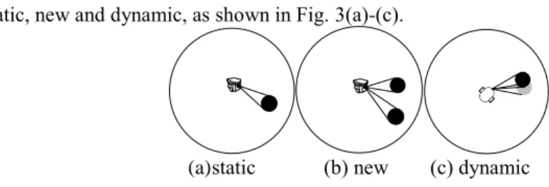
2.3 Identify the type of an obstacle

An obstacle chain, Ob_chain = {O1(t), O2(t),…, Ok(t)}, is produced after clustering. For each obstacle, we can calculate the center Zk(t), the grid area Sk(t), and the coincidence ξk(t), respectively. Then the spatial correlation can be calculated, and the obstacle with maximum spatial correlation ςk(t),max can be obtained. Three possible obstacle types are

static, new and dynamic, as shown in Fig. 3(a)-(c).

(a) static (b) new (c) dynamic Fig. 3 Different types of obstacles

Two thresholds θς1 and θ ς2 of the spatial correlation are set for distinguishing a new or a static obstacle. Fig. 3 (a) shows a static obstacle, when ςk,max > θς2,; Fig. 3 (b) shows a new obstacle, when ςk,max < θ ς1,; Fig. 3 (c) shows a dynamic obstacle. When the value ςk,max ∊ [θ ς1, θ ς2], then the obstacle is possibly a dynamic obstacle. It will be further evaluated in terms of center distance δ (0 ≤ δ <rw) between two obstacles and the coincidence ξk(t). A threshold θδ is set to distinguish static and dynamic obstacle. If δ< θδ, the obstacle is stat-ic, otherwise, the obstacle is evaluated in terms of the coincidence ξk(t). A threshold θξ is set as well. If ξk(t) ≥ θξ , then the obstacle is static, otherwise, it is dynamic. Fig.4 illus-trates the process of the obstacle classification using a simple decision tree.

2.4 Movement of a dynamic obstacle

The dynamic obstacles are further analyzed to calculate the speed and angle of their movement (Fig.5). Assume the time interval of two rounds of laser scanning is T. We can catch up the global coordinates of a moving robot at time t and t-T, R(x(t), y(t)) and R(x( t-T), y(t-T)). Hence, we always can calculate the global coordinates of an obstacle, Ok(xk(t), yk(t)) and Ok(xk(t-T), yk(t-T)), given the values from laser beams at time t and t-T, using Eq. (1).

Fig. 4 The decision tree of obstacle classification Fig. 5 Motion process of an obstacle

The moving distance do, speed vo and the direction angle αo of the dynamic obstacle from t-T to t can be calculated with Eqs. (13)-(15). Similarly, the distance dR, speed vR and the direction angle αR of the moving robot from time t-T to t can be calculated as well.

k k< 1 k> 2 k [ 1, 2] static new dynamic do dR (t T) Ok(xk(t),yk(t)) Ok(xk(t T),yk(t T)) 0 t R(x(t),y(t)) R(x(t T),y(t T))

(13) (14) (15)

According to the states of the robot and the obstacle, the robot can predict the potential collisions ahead. There are six scenarios, when a robot is moving in its surrounding envi-ronment: (1) a static obstacle is in front of the robot, where the collision is just at the point of obstacle; (2) an obstacle at the probing area, moving at a faster speed than the robot, could pass the path before robot arrives the potential collision point; (3) an obstacle at the probing area, moving slower than the robot, has not arrived at the path, when robot arrives the potential collision point; (4) the robot and the obstacle may collide at the crossing point between robot’s path and obstacle’s path when the current speed, distance, and posi-tion of the robot and the obstacle make them arrive the point at the same time; (5) the robot and the obstacle are running in opposite direction, hence, the robot and the obstacle could collide at a point between the robot and the obstacle; (6) the robot is running in the same direction as an obstacle but is faster than the obstacle, then the robot may collide with the obstacle at some time.

4. Avoiding obstacle collision

We use the classic local path avoidance algorithm --- Morphin algorithm [15,16] to im-plement the path planning. As shown in Fig. 6, an obstacle that may collide with the robot is detected, a few alternative paths to avoid the obstacle are set in the front of the robot, and the optimal obstacle avoidance path is selected according to the current state of the robot and the evaluation function of the alternative paths.

In the Morphin algorithm, the robot is always assumed to face the obstacle (e.g. scenarios (1), (5), (6)). Hence, we can connect the robot's current position and the center of the ob-stacle to form a centerline, and draw several arcs on the left and right sides of the center-line and evaluate each arc by using Eq. (16).

Fig. 6. Alternative paths in the Morphin algorithm

𝑦 = {∞, 𝑡ℎ𝑒⁡𝑜𝑏𝑠𝑡𝑎𝑐𝑙𝑒⁡𝑖𝑠⁡𝑎𝑏𝑜𝑣𝑒⁡𝑡ℎ𝑒⁡𝑎𝑟𝑐,_𝜀 1𝑃 + 𝜀2𝑀 + 𝜀3∆𝐿 + 𝜀4𝑊, 𝑜𝑡ℎ𝑒𝑟𝑠. (16)



 



where, P represents the length of each arc path; M represents the inflection point parame-ter of each arc path; ΔL represents the average distance from each grid point to the sub-target point through which the arc passes; W represents the arc endpoint and the number of times the sub-target points intersect the obstacle grid; ε1, ε2, ε3, ε4 are the weights of the items, respectively. When the obstacle is above the arc, the value of the evaluation func-tion y is infinite, and the arc with the smallest y value represents the local optimal path. For more details about the Morphin algorithm, please refer to the research in [15][16]. In the scenarios (1), (5) and (6), a collision could occur, hence, the Morphin algorithm is called to update the robot’s path with the optimal path for collision avoidance. In the sce-narios (2) and (3), no collision could occur, hence, the robot will not take any measures and continue to run. In the scenario (4), the robot will stop running until the obstacle pass-es the predicted collision point.

3

Experiments

To validate the effectiveness of the proposed ATCM system, we conducted some ments for robot moving from a specific starting point to a specific target. The experi-mental platform is MATLAB. All parameters in the experiments are set with trial and error method. The simulation environment is set to a 20x20 grid map with many obsta-cles. Grid resolution r = 500mm. The radius rw of the dynamic window is set to 8 grids. As all obstacles added to the grid map have a regular shape, the adaptive rate λ of the threshold Θ is set to 1.2; for simplicity, the parameters in the obstacle classification tree (Fig.4) are set as: θς1=0.30, θς2=0.7, θδ=0.4, θξ=0.5, respectively. The parameters (ε1~ ε4) of Morphin Algorithm are set to 1, 1, 1.3 and 0.6, as in [16]. Three experiments are con-ducted: (1) without dynamic obstacles; (2) adding some dynamic obstacles in the grid environment; (3) a mixed case with static and dynamic obstacles.

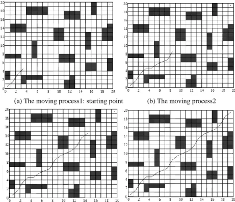
3.1 Without dynamic obstacles

Fig. 7 shows the local path planning process of a mobile robot when there are no tem-porary obstacles in the environment. The mobile robot does not find any dynamic obsta-cles, except the fixed obstacles in the rolling window in the grid environment. Using the rolling window algorithm, each rolling step draws the rolling window centered on the current position and updates the window map. The mobile robot moves towards the next step. The local sub-targets are rolled forward step by step, and finally a trajectory is formed from the starting point to the target.

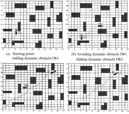
3.2 Adding instantly dynamic obstacles

Dynamic obstacle avoidance increases the computing complexity, as the robot needs to predict potential collision point in terms of the dynamics of the obstacle. Fig. 8 shows the simulation of the local path planning process by adding three types of dynamic obstacles to the grid map. The mobile robot starts from the starting point and relies on the sensor, and identifies the dynamic obstacle Ob1 in the current window. The robot calculates the

(a) The moving process1: starting point (b) The moving process2

(c) The moving process3 (d) The moving process4

motion trajectory of Ob1, and predicts that it will not collide with Ob1. Hence, it will keep the original speed and moving direction. When the mobile robot moves and finds Ob2, a moving obstacle, and predicts that it could collide with Ob2. Hence, it stays in the place for a while until Ob2 passes the collision point. After the dynamic obstacle passes the collision point, the robot generates local sub-goal in the current window and moves. When the robot detects the dynamic obstacle Ob3 from the opposite side, the collision is una-voidable, and the collision point is predicted, then the robot calls the Morphin algorithm to get an optimal path, and moves following the path until reaching the specified target.

Fig. 7 Local path planning process without dynamic obstacles

3.3 A mixed case

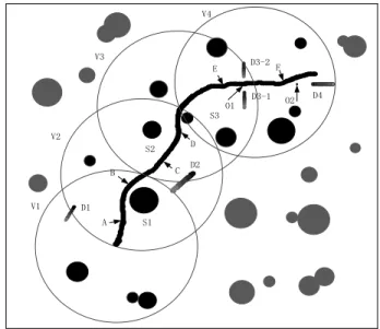
The simulation results are shown in Fig. 9. In a real case, the circular window is up-dated in real time, and the center trajectory of the dynamic circular window is the trajecto-ry of the robot. For demonstration, V1, V2, V3 and V4 denote circular windows, S1, S2, S3 and S4 denote detected static obstacles, and D1, D2, D3-1, D3-2, D4 represent the detected dynamic obstacles. At C, E, F, the robot detects dynamic obstacles, and at A and D, the

robot detects the static obstacles, respectively. Table 1 provides the speeds and angles of the four detected dynamic obstacles at different positions in the grid map. Figure 10 shows the obstacle avoidance process in the mixed case.

Fig. 8 Local path planning process for adding instantly dynamic obstacles

Table 1 Movement speed and angle of obstacle

D1 D2 D3 D4

v 450mm/s 760mm/s 510mm/s 805mm/s

α 80.83˚ 62.47 ˚ 91.05 ˚ 180.09

As shown in Fig. 9, the robot moves within the V1 window and builds a dynamic win-dow map, where, the robot detects obstacle S1 at point A and calls Morphin algorithm to avoid the obstacle S1. In the phase from A to B, the moving obstacle D1 is recognised at the speed of 450mm/s and the angle of 80.83˚; once the robot moves beyond the effective area of V1, a circular window of V2 is constructed immediately, and the moving obstacle

(a) Starting point:

Adding dynamic obstacle Ob1 (b) Avoiding dynamic obstacle Ob1 _{Adding dynamic obstacle Ob2}

(c) Avoiding dynamic obstacle Ob2 Adding dynamic obstacle Ob3

(d) Avoiding dynamic obstacle Ob3 Reaching the target

D2 is detected at the phase from C to D, with the speed of 760mm/s and the angle of 62.47 ˚; a static obstacle S3 is detected at D, hence, the Morphin algorithm is called im-mediately. Similarly, beyond the valid area of V2, a circular window of V3 is constructed. When reaching at E, the robot obtains the information that obstacle D3-1 is running at a speed of 510 mm/s and the angle of 91.05 ˚, and predicts that a collision could occur at O1. In this case, the robot will stop, and wait for the detected obstacle D3-1 running away from the collision point to become D3-2, and then start running again. In the V4 window, at F, an opposite obstacle is detected, running at the speed of 805mm/s and the angle of 180.05˚, which would produce a collision at O2 if robot does not change its direction im-mediately. In this case, the robot calls the Morphin algorithm immediately to change the path, thus to avoid the collision.

4

Conclusions

This research provided a comprehensive obstacle avoiding system, ATCM, for a mo-bile robot in unknown environment. A dynamic circular window is updated in real time during the navigation. The laser data in the circular window are clustered with the adap-tive threshold nearest neighbor clustering algorithm. Three types of obstacles can be clas-sified in terms of three parameters, spatial correlation, center distance, and coincidence of two obstacles. Then potential collision with detected static and dynamic obstacles is pre-dicted. The Morphin algorithm is applied to find an alternative path when robot detects a potential collision ahead. The simulation results show that the mobile robot can effective-ly detect obstacles, predict potential collision, and avoid obstacles. The future work is to apply the ATCM system to laboratory robots, and improve the system.

v V1 V2 V3 S1 S2 S3 D1 D2 D3-1 D3-2 D4 A D F E B C v v V4 O1 O2

Acknowledgments

This work was supported by 2018 Natural Science Foundation of Anhui, China (1808085QF215), 2018 Foundation for Distinguished Young Talents in Higher Education of Anhui, China (gxyqZD2018050) and Anhui Key Research and Development Programs (Foreign Scientific and Technological Cooperation, 1804b06020375).

References

1. WANG J L, ZHOU J, GAO H, et al. Obstacle Avoidance Method for Mobile Robots Based on the Identification of Local Environment Shape Features. Information and Control, 2015, 44(1):91-98.

2. LUO J, LIU C, LIU F. Piloting-following formation and obstacle avoidance control of multiple mobile robots. CAAI Transactions on Intelligent Systems, 12(02):1-10, (2017).

3. ZHANG Q, WANG P, CHEN Z. Velocity space based concurrent obstacle avoidance and tra-jectory tracking for moble robots. Control and Decision, 32(02): 358-362, (2017).

4. ZHANG Q, YANG X, LIU T, et al. Design of a Smart Visual Sensor Based on Fast Template Matching. Design of a Smart Visual Sensor Based on Fast Template Matching, Chinese Journal of Sensors and Actuators, 26(8): 1039-1044, (2013).

5. WANG Z, CUI X, HOU C. Analysis and Countermeasures to the Problem of Ultrasonic Sensor Receives the Ultrasonic Signal Asymmetric[J]. Chinese Journal of Sensors and Actuators, 28(1): 81-85, (2015)

6. WANG M, FAN Y, WANG X, et al. Design of infrared FPA detector simulator. Laser and In-frared, 46(12): 1481-1485, (2016).

7. ZHANG Y, XU J, CHEN L, et al. Design of terrain recognition system based on laser distance sensor. Laser and Infrared, 46(03): 265-270, (2016).

8. ZHANG D, LI W, WU H, et al. Mobile Robot Adaptive Navigation in Dynamic Scenarios Based on Learning Mechanism. Information and Control, 45(05): 521-529, (2016).

9. XIN Y, LIANG H, MEI T, et al. Dynamic Obstacle Detection and Representation Approach for Unmanned Vehicles Based on Laser Sensor. Robot, 36(6): 654-661, (2014).

10. HUANG R, LIANG H, CHEN J, et al. Lidar Based Dynamic Obstacle Detection, Tracking and Recognition Method for Driverless Cars. Robot, 38(4): 437-443, 2016.

11. LIU J, YAN Q, TANG Z. Simulation Research on Obstacle Avoidance Planning for Mobile Robot Based on Laser Radar. Computer Engineering, 41(4): 306-310, (2015).

12. YANG Y, HAN F, CAO Z, et al. Laser Sensor Based Dynamic Fitting Strategy for Obstacle Avoidance Control and Simulation. Journal of System Simulation, 25(4): 118-122, (2013). 13. ZHONG X, PENG X, ZHOU J, Detection of moving obstacles for mobile robot using laser

sensor, the 20th ChineseControl Conference (CCC), Yantai, China, 22-24 July 2011.

14. ZHU J, ZHOU Y, WANG C, et al. Grid Map Merging Approach Based on Image Registration. Acta Automatica Sinica, 41(2): 285-294, (2015).

15. ZHU-GE C, TANG Z, SHI Z. UGV local path planning algorithm based on multilayer Morphin search tree. Robot, 04: 491-497, (2014).

16. WAN X, HU W, ZHENG B, et al. Robot path planning method based on improved ant colony algorithm and Morphin algorithm.Science and Technology Review, 33 (3): 84-89, (2015).