Adaptive Scheduling over a Wireless Channel under
Constrained Jamming
?Antonio Fern´andez Anta1, Chryssis Georgiou2, and Elli Zavou1,3
1
Institute IMDEA Networks, Madrid, Spain,
2
University of Cyprus, Nicosia, Cyprus,
3
Universidad Carlos III de Madrid, Madrid, Spain
Abstract. We consider a wireless channel between a single pair of stations (sender and receiver) that is being “watched” and disrupted by a malicious, adversarial jam-mer. The sender’s objective is to transmit as much useful data as possible, over the channel, despite the jams that are caused by the adversary. The data is transmitted as the payload of packets, and becomes useless if the packet is jammed. In this work, we develop deterministic scheduling algorithms that decide the lengths of the packets to be sent, in order to maximize the total payload successfully transmitted over periodT
in the presence of up tofpacket jams,useful payload.
We first consider the case where all packets must be of the same length and compute the optimal packet length that leads to the best possible useful payload. Then, we con-sider adaptive algorithms; ones that change the packet length based on the feedback on jammed packets received. We propose an optimal scheduling algorithm that is es-sentially a recursive algorithm that calculates the length of the next packet to transmit based on the packet errors that have occurred up to that point. We make a thorough non trivial analysis for the algorithm and discuss how our solutions could be used to solve a more general problem than the one we consider.
Keywords: Packet scheduling, Wireless Channel, Unreliable communication, Adversarial jamming
1
Introduction
Motivation and prior work. Transmitting data over wireless media is becoming increas-ingly popular, especially with the dramatic increase of the use of mobile devices (e.g., smart phones). A major challenge that needs to be addressed is to cope with disruptions of the communication over such media, especially when these disruptions are caused intention-ally, e.g., by jamming devices. Several research efforts have been made in addressing this challenge under different assumptions and constraints (e.g.,[1–6, 9–12]).
In a recent work [2], we have initiated the investigation of the following problem: We consider a wireless channel between a single pair of stations (sender and receiver) that is being “watched” and disrupted by a malicious, adversarial jammer. The sender’s objective is to transmit as much useful data as possible, over the channel, despite the jams that are caused
?This research was supported in part by Ministerio de Econom´ıa y Competitividad grant
by the adversary. The data is transmitted as the payload ofpackets, and becomes useless if the packet is jammed. The adversary has complete knowledge of the packet scheduling algorithm and it decides on how to jam the channel dynamically. However, the jamming power of the adversary is constrained by two parameters,ρandσ, whose values depend on technological aspects. The parameterσrepresents the maximum number of “error tokens” available for the adversary to use at any point in time, andρrepresents the rate at which new error tokens become available (one at a time). Each error token models the ability of the adversary to jam one packet. This adversarial model could represent a jamming entity with limited resource of rechargeable energy, e.g., malicious mobile devices or battery-operated military drones. In these cases,σrepresents the capacity of the battery (in packets that can be jammed) andρthe rate at which the battery can be recharged (for instance, with solar cells). To evaluate scheduling algorithms, two efficiency measures are used: thetransmission time, to completely send a fixed pre-defined amount of data, and thegoodput ratio(successful transmission rate) achieved to do so, which intuitively are reversely proportional.
Under this model, we first showed in [2] upper and lower bounds on the transmission time and goodput when the sender sends packets of the same length throughout the execu-tion (uniform case); in this case the scheduling policy does not take into account the history of jams. Then, considering the caseσ= 1, we proposed an adaptive scheduling algorithm that changes the packet length based on the feedback on jammed packets received, and showed that it can achieve better goodput and transmission time with respect to the uniform case, for most values ofρ. However, the analysis technique used for the caseσ= 1turned out not to be easily generalized for cases whereσ >1.
In order to better understand the above problem and lay the groundwork for obtaining its optimal solutions, in this work we consider a simpler, more “static” version of the problem. In particular, we focus on a specific time interval of lengthT, and instead of assuming that new error tokens are continuously arriving we assume a fixed number of error tokensf. As before, the sender’s objective is to correctly transmit the maximum amount of data, in the form of packets, under the jamming of the adversary. Now, the adversary is constrained only by parameterf, which is the maximum number of errors (packet jams) it can introduce in the corresponding intervalT and are available from the very beginning of the interval. There-fore, givenTandf as input, we would like to maximize the totaluseful payloadtransmitted within the interval of interest. (Our modeling assumptions are detailed in Section 2.)
We plan to use the results obtained for this problem to derive solutions of the continuous version of [2], but we believe that this static problem is a fundamental and challenging problem and hence of interest by itself.
Contributions.We provide a comprehensive solution to the abovementioned problem (static version). Specifically:
– We first consider the case where the scheduling algorithm is restricted in sending packets of the same length (uniform case); this could be due to limitations in the communication protocol or the sender’s specification (Section 3). Given a period of lengthT and up tof packet jams, we show that the optimal packet length isp∗≈p
T /f that leads to optimal useful payloadT+f−2pT /f. In the case the adversary does not cause any packet error in the interval of timeT, we show that the useful payload achieved by uniform packets of lengthp∗isT −p
– Then, we devise adaptive scheduling algorithms, that is, algorithms that change the packet length based on the feedback on jammed packets received. We start by first con-sidering the case off = 1(Section 4). We devise algorithm ADP(T,1)and prove its op-timality. We show that the algorithm achieves optimal useful payload of i−i1T−i+1
2 + 1 i, whereiis the integer such thatT ∈h(i−21)i + 1,i(i+1)2 + 1.
Algorithm ADP(T,1) chooses the lengthp of the first packet to be transmitted as a function ofT. If the packet is jammed then it transmits a second packet of lengthT−p which is now guaranteed not to be jammed. If the first packet goes through, then the algorithm is invoked recursively as ADP(T−p,1).
– Next, we generalize algorithm ADP(T,1)into algorithm ADP(T,f)and show that it obtains optimal useful payload for anyf(Section 5). Algorithm ADP(T,f)is essentially a recursive algorithm that also begins by choosing length pof the first packet to be transmitted as a function ofT(a different function from that of ADP(T,1)). If the packet is jammed, the adversary (unlike in the case off = 1) still has error tokens that it can use. Therefore, instead of sending a packet that spans the rest of the interval, ADP(T,f) makes the recursive call ADP(T−p,f −1). If the packet is not jammed, then it makes a recursive call to ADP(T−p,f).
Although the above algorithmic approach is natural, the choice of the length pof the packet to be sent as well as the algorithm’s analysis of optimality, are nontrivial. – Finally, we discuss and compare the version of the problem considered in this work
(static) with the one of [2] (continuous) and draw interesting conclusions (Section 6). Related work. Several studies have investigated the effect of jamming in wireless chan-nels. For example, Thuente et al. [12] studied the effects of different jamming techniques in wireless networks and the trade-off with their energy efficiency. Their study includes from trivial/continuous to periodic and intelligent jamming (taking into consideration the size of packets being transmitted). Pelechrinis et al. [6] present a detailed survey of the De-nial of Service attacks in wireless networks. They present the various techniques used to achieve malicious behaviors and describe methodologies for their detection as well as for the network’s protection from the jamming attacks. Dolev et al. [4] present a survey of sev-eral existing results in adversarial interference environments in the unlicensed bands of the radio spectrum, discussing their vulnerability.
the adversary can jam at most(1−ε)T of the time steps in that period. In our case, the adversary, within a time periodT,can causef channel jams, wherefdoes not correspond to a fraction of time, but on the number of packets it can corrupt. Other differences is that they considern nodes transmitting over the channel (hence, they deal with transmission collisions) and their objective is to optimize throughput over the non-jammed time periods. Finally, Gilbert et al. [5] investigated the impact on the communication delay between two honest nodes that a third malicious, energy-constraint node can have. In particular, the three nodes share a time-slotted single-hop wireless radio channel and the two honest nodes begin with a value to communicate. The malicious node wishes to prevent them from com-municating for as long as it can, by broadcasting messages. However, it is allowed to broad-cast up toβmessages. This is similar to the restriction we impose in our work, by allowing the adversary to cause up tof packet errors. The setting and objectives of the work [5], though, are different. First they show a tight bound on the number of rounds that the mali-cious node can delay the communication between the two honest entities:2β+Θ(log|V|) rounds, whereV is the set of possible values the two honest nodes may communicate. Then, they study the implication of this bound on more generaln-node problems, such as reliable broadcast and leader election.
2
Model
We now present in detail the model considered in this paper.
Network setting. We consider an unreliable wireless channel that connects two end stations: a sender and a receiver. The sender has data to be transmitted to the receiver over a fixed time intervalT, which is sent as the payload of the packets scheduled. However, the channel is prone to instantaneous jams. Hence, using anonline scheduling algorithm[7, 8], the sender needs to decide the length of the packets to be sent in in the time interval, taking or not into consideration the history of transmissions and jams that already occurred. The objective of the sender is to provide the receiver with as much data as possible over the period of time T, despite channel jams.
As in [2], each packet sent across the channel consists of aheaderof a fixed predefined sizehand apayloadof lengthlchosen by the algorithm; the total length of the packet is p = h+l. For simplicity we assume thath = 1, i.e.,p = l+ 1(we assumel to be a real number). Recall that the payload corresponds to the useful data sent across the channel. In addition, we assume that the transmission time of each packet is equal to its length; the channel has a constant transmission rate.
Efficiency measures. As in [2], we consider two efficiency measures,useful payloadand goodput rate. The useful payload, is the sum of payloads of the successfully transmitted packets within a time interval of lengthT, under anyf-size error patternE. The goodput rate, is the corresponding ratio of the useful payload sent during the interval and is of interest mostly for the continuous version of the model presented in [2].
More formally, we denote by UPA(T,f, E)the useful payload (payload correctly re-ceived) when using scheduling algorithmA in an interval of lengthT against an adver-sary of powerf that uses error patternE. For a fixed algorithmA, its useful payload is then simply UPA(T,f) = minE∈E(f)UPA(T,f, E), where E(f) is the set of all possi-ble error patterns with at mostf jams. From this, we define the optimal useful payload as UP∗(T,f) = maxAUPA(T,f).
The goodput metric is defined similarly, by simply dividing the useful payload by the length of the interval. More precisely, when using scheduling algorithmA in an interval of lengthT against an adversary of powerf that uses error patternE, the goodput rate is GA(T,f, E) =UPA(T,f, E)/T, the goodput of algorithmAisGA(T,f) =UPA(T,f)/T, and the optimal goodput isG∗(T,f) =UP∗(T,f)/T.
Feedback mechanism. Following [1, 2], we consider instantaneous feedback. In particular, at the time a packet is successfully received by the receiver, a notification/acknowledgement message is immediately received by the sender. If such a message is not received by the sender, then it considers the packet to be jammed. We assume that the notification packets cannot be jammed by the errors in the channel because of their relatively small size. Remark: Observe that ifT ≤f, then the adversary can jam all packets sent in the interval and no useful data will be received. Therefore, from this point onward we focus only in time periods that are initially of lengthT >f.
3
Uniform Packets
We first consider the case in which all the packets scheduled are of the same length. Having to use uniform packets may be a requirement due to limitations in the communication proto-col, or the sender’s specifications. In this case, the following result gives the uniform packet length that has to be used in order to maximize the minimum useful payload. (Note that the approximations below are due to floors and ceilings; these approximations get closer to equality asTf grows.)
Theorem 1. LetU(p)denote the algorithm that only uses uniform packets of lengthp. In an interval of length T and maximum number of errorsf, the optimal packet length for these algorithms isp∗ ≈p
T /f that achieves useful payload UPU(p∗)(T,f) ≈ T+f −
2√Tf. When the adversary causes no jamming, the useful payload achieved byU(p∗)is UP∗U(p∗)(T,f,∅)≈T−
√
Tf.
Proof. Let us denote bynthe number of uniform packets of lengthp= T
Deriving this expression with respect ton, we get ∂UPU(n)(T,f)
∂n =
f T n2 −1,
which implies that UPU(n)(T,f)is maximized forn =
√
Tf. Moreover, the derivative is positive forn < √Tf and negative forn > √Tf, which implies that the useful payload is strictly increasing on the left ofn = √Tf and strictly decreasing on the right. From this, we get that (1) there is no othernthat maximizes the useful payload, and (2) since the number of packets has to be an integer value, the only two candidates for the optimal number of packetsn∗areb√Tfcandd√Tfe. Hence the value of these two that maximizes the useful payload is the optimal numbern∗. From this, and the fact thatp= Tn, we get that p∗≈p
T /f, as claimed.
Then, the optimal number of packetsn∗gives optimal useful payload UPU(n∗)(T,f) =
(n∗ −f)(nT∗ −1) ≈ T +f −2 √
Tf, as claimed. Finally, when n∗ packets are used, and no packet is jammed by the adversary, the useful payload is maximized reaching UPU(n∗)(T,f,∅) =n∗(T
n∗−1)≈T− √
Tf, as desired. ut
Corollary 1. The optimal achievable goodput rate isGU(p∗)(T,f)≈
1−pf/T 2
.
4
Optimal Algorithm for
f
= 1
In this section, we turn our focus on the case of a single error token available to the adversary for an interval of lengthT. We give an adaptive algorithm, named ADP(T,1), and prove its optimality. By doing so, we hope to give an intuition to the reader for how the general optimal algorithm, for any number of error tokens, works.
Algorithm 1 ADP(T,1)
If T ∈[1,2)then
Sendpacket with length p=T
else
Let ibe the integer such that T ∈h(i−1)i
2 + 1,
i(i+1) 2 + 1
Let α=i−2, andβ= (i−21)i−1
Sendpacket πwith length p= Tα++2β =T−1
i + i−1
2
If packet πis jammed then
Sendpacket with length p0=T−p
else
Call ADP(T−p,1)
The detailed description of the algorithm is given as Algorithm 1. Let us fix the interval lengthT ≥1, and letibe the integer such thatT ∈h(i−21)i + 1,i(i+1)2 + 1, as described in the above pseudocode. Let us also define parametersα = i−2 andβ = (i−21)i −1, packet lengthp= Tα+2+β, and interval lengthT0=T−p. We first present the following two lemmas that are used to show the optimality of Algorithm ADP(T,1).
Lemma 1. Interval lengthT0 = T −pis such thatT0 ∈ h(j−21)j + 1,j(j+1)2 + 1for j=i−1, whereiis an integer such thati≥1.
Proof. Replacing the values ofαandβin the calculation ofT0=T−p,
T0= (α+ 1)T−β
α+ 2 =
(i−2 + 1)T−(i−21)i −1
i−2 + 2 =
(i−1)T−(i−21)i+ 1
i .
Now, using the fact thatT ≥(i−21)i+ 1, we have
T0≥
(i−1)1 +(i−21)i−(i−21)i+ 1
i =· · ·=
(i−1)(i−2)
2 + 1.
Similarly, using the fact thatT <i(i+1)2 + 1, we have
T0<
(i−1)1 +i(i+1)2 −(i−21)i+ 1
i =· · ·=
(i−1)i
2 + 1.
Settingj=i−1in both cases, we haveT0∈h(j−21)j + 1,j(j+1)2 + 1as claimed. ut
Lemma 2. LetT ≥2and assume that UPADP(T0,1) = αTα+10−β, whereT0=T−p. Then, Algorithm ADP(T,1)achieves useful payload UPADP(T,1) = (α+1)Tα+2−(β+α+2).
Proof. SinceT ≥2, that Algorithm ADP(T,1)schedules first a packetπwith lengthp= T+β
α+2. Ifπis jammed, then a packet of length equal to the rest of the interval, i.e.,T
0 =T−p,
can be sent successfully, and hence the useful payload will be UPADP(T,1) =T−Tα+2+β−
1 = (α+1)Tα+2−(β+α+2).
Otherwise, ifπis not jammed, the useful payload is obtained as UPADP(T,1) = p−
1 +UPADP(T0,1) =p−1 + αTα+10−β =p−1 +α(Tα+1−p)−β = (α+1)Tα+2−(β+α+2). In both cases, the useful payload is as claimed, which completes the proof. ut
Theorem 2. Given an interval of length T ≥ 1, Algorithm ADP(T,1)achieves optimal useful payload UP∗(T,1) = i−1
i T − i+1
2 + 1
i, where i is the integer such that T ∈
h(i
−1)i 2 + 1,
i(i+1) 2 + 1
.
and can be jammed by the adversary. Observe that in this case at most one packet can in fact be sent in the interval. This matches the claim that ADP(T,1)achieves optimal useful payload UP∗(T,1) = 0in this case.
Let us now consider any interval length T ≥ 2, which implies i ≥ 2. Then, from Lemma 1, interval length T0 = T −p ∈ h(j−21)j+ 1,j(j+1)2 + 1 for j = i−1. By induction hypothesis, UPADP(T0,1) = UP∗(T0,1) = j−j1T − j+12 +1j = αTα+10−β, and from Lemma 2 we have that UPADP(T,1) = (α+1)Tα+2−(β+α+2)= i−i1T−i+1
2 + 1 i. To show that the useful payload achieved by ADP is optimal for this caseT ≥ 2, consider an algorithmAthat follows one of the following approaches:
(a) First sends a packetπ0of lengthp0> Tα+2+β. We assume then that the adversary jamsπ0. The length of the rest of the interval isT−p0 < T −T+βα+2. Hence the useful payload will be
UPA(T,1)< T−T+β
α+ 2 −1 =
(α+ 1)T−(β+α+ 2)
α+ 2 =UPADP(T,1). (b) First sends a packetπ0of lengthp0 <Tα+2+β,p0≥1. Then the adversary does not jamπ0. The rest of the interval has lengthT −p0 =T0+ (p−p0) > T0. We consider two cases (from Lemma 1 no other case is possible):
Case (b).1: T −p0 = T0 + (p−p0) ∈ h(j−21)j+ 1,j(j+1)2 + 1 forj = i−1. Then, by induction hypothesis, UP∗(T0 + (p−p0),1) = j−j1(T0 + (p−p0))− j+12 + 1j <
j−1 j T
0−j+1 2 +
1
j + (p−p
0) =UP∗(T0,1) + (p−p0). Hence,
UPA(T,1)≤p0−1 +UP∗(T0+ (p−p0),1)< p0−1 +UP∗(T0,1) + (p−p0) =p−1 +UP∗(T0,1) =UPADP(T,1).
Case (b).2:T −p0=T0+ (p−p0)∈h(i−21)i+ 1,i(i+1)2 + 1. In this case,
UPA(T,1)≤p0−1 +UP∗(T−p0,1) =p0−1 + i−1 i (T−p
0)−i+ 1
2 +
1 i
< i−1 i T−
i+ 1
2 +
1
i =UPADP(T,1),
where the first equality follows from induction hypothesis, and the second inequality follows from the fact thatp0 < i(derived fromp0 < Tα+2+β, the definition ofαandβ, and the fact thatT < i(i+1)2 + 1).
Hence, in none of the two cases, neither (a) nor (b), AlgorithmAwas able to achieve a higher useful payload than ADP, which implies that the latter achieves optimality. ut
5
Optimal Algorithm for ANY
f
>
1
of ADP(T,f)forf >1is similar to that of ADP(T,1), with a couple of differences. First, in this case it is not possible to explicitly give the lengthpof the first packetπsent (values ofα,β, andγ) whenT ≥f + 1(see Theorem 3). Second, ifπis jammed, the adversary still has some error tokens that it can use. Hence, instead of sending a packet that spans the rest of the interval, ADP(T,f)makes the call ADP(T−p,f−1), which could be recursive iff >2, or a call to the algorithm ADP(T−p,1)(see Algorithm 1), iff = 2. It will not be surprising then that the proof of optimality of the algorithm ADP(T,f)will use induction onf.
Algorithm 2 ADP(T,f), forf >1 If T <f + 1then
Sendpacket with length p=T
else
Sendpacket πwith length p= αT+β
γ //α, βandγdepend onT; see Theorem 3
If packet πis jammed then Call ADP(T−p,f −1) else
Call ADP(T−p,f)
Let us first prove some observations that hold for any optimal algorithm OPT, to be used later in the analysis of Algorithm ADP(T, f).
Observation 1 The useful payload of an optimal algorithm OPT, follows a non-decreasing function with respect to the length of the interval of interest, T, when there are f ≥ 0 available errors, i.e., UP∗(T,f)≤UP∗(T+δ,f), forδ >0.
Proof. Let us consider an optimal algorithm OPT that achieves optimal useful payload UP∗(T,f) = α, for an interval of length T andf error tokens available within the in-terval. Now let us construct an algorithm A, that for interval lengthT +δ initially uses the exact same approach as OPT forT; choosing the same packet lengths OPT does dur-ing the initialT time of the interval. This means that it has at least the same useful pay-load as OPT for T, i.e., UPA(T +δ,f) ≥ α. Since OPT is the optimal algorithm, it must achieve at least the same useful payload asAfor the interval of lengthT +δ, i.e., UP∗(T+δ,f)≥UPA(T+δ,f). Hence, UP∗(T,f)≤UP∗(T+δ,f)as claimed. ut
Observation 2 The useful payload of an optimal algorithm OPT, follows a non-increasing function with respect to the number of available errors in an interval of length T, i.e., UP∗(T,f)≤UP∗(T,f −1), wheref ≥1.
Proof. Let us consider an optimal algorithm OPT, with a useful payload UP∗(T,f) =βfor an interval lengthT withf errors available. Then, let us construct an algorithmA, that for f −1error tokens during the same interval lengthT, uses the exact approach as OPT forf errors; choosing the same packet lengths untilf −1error tokens are used by the adversary. Then, it schedules one packet equal to the size of the remaining interval. This means that it has at least the same useful payload as OPT does forf errors, UPA(T,f −1)≥β. And since OPT is the optimal algorithm, it must achieve at least the same useful payload for the same interval andf −1errors, i.e., UP∗(T,f −1)≥UPA(T,f −1). Hence, UP∗(T,f)≤
Lemma 3. There is an optimal algorithm OPT that is work-conserving. I.e.,∀T and ∀f, there is an optimal work-conserving strategy deciding the packet lengths.
Proof. Assume by contradiction that there is some combination of interval and number of error tokens(T,f), for which no work-conserving scheduling strategy is optimal. We choose the smallest suchT and consider the following:
(1) There is an optimal strategy for this pair ofTandf that does not send any packet during the interval. Hence the optimal useful payload is zero, UP∗(T,f) = 0. In this case, sending one packet that spans the whole interval will lead to the same payload.
(2) There is a strategy that waits for∆time at the beginning of the interval before sending a packet of lengthp. This packet can be jammed. Therefore,
UP∗(T,f) = min{UP∗(T−∆−p,f −1), p−1 +UP∗(T −∆−p,f)} ≤min{UP∗(T−p,f −1), p−1 +UP∗(T−p,f)}.
Where the inequality follows from Observation 1. The right side of the inequality is the use-ful payload obtained by the strategy that does not wait the∆period, but instead schedules the packet of lengthpat the beginning of the interval (which is work-conserving). Since both cases lead to a contradiction, the claim follows. ut
Lemma 4. The optimal useful payload is a continuous function with respect to the length of the interval,T, when there aref ≥1errors available.
Proof. Assume by contradiction that the optimal useful payload is not a continuous func-tion. This means that there is an interval lengthTfor which the following holds:lim
→0UP
∗(T−
,f) < UP∗(T,f). Let us fix parameter > 0, and observe the behavior of a work-conserving optimal algorithm OPT for interval lengths T and T − (such an algorithm exists by Lemma 3). Let us then denote bypOandpthe lengths of the first packet sched-uled by OPT in each case respectively. These packets can be jammed or not. We observe that
UP∗(T−,f) = min{UP∗(T−−p,f −1), p−1 +UP∗(T−−p,f)} (1) UP∗(T,f) = min{UP∗(T−pO,f −1), pO−1 +UP∗(T −pO,f)} (2) However, if we construct an alternative algorithmAthat chooses a packet of lengthp00 = pO−in the case of interval of lengthT−, and works as OPT for smaller interval lengths, then
UPA(T−,f) = min{UP∗(T−pO,f−1), pO−−1 +UP∗(T−pO,f)} ≥UP∗(T,f)−. Since UP∗(T−,f)≥UPA(T−,f), it is then trivial to conclude thatlim
→0UP
∗(T−,f) =
UP∗(T,f), which is a contradiction. Hence the optimal useful payload is a continuous func-tion with respect to the length of the interval, as claimed. ut
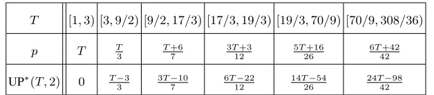
calls is the optimal value UP∗(T0, j). Then, ADP(T,f)chooses as length of packetπthe smallest valuep∈[1, T]that satisfies the equality UP∗(T−p,f−1) =p−1+UP∗(T−p,f). Table 1 shows the values ofpchosen for some interval lengthsTwhenf = 2. It also shows the useful payload achieved by the algorithm using these values ofp.
T [1,3) [3,9/2) [9/2,17/3) [17/3,19/3) [19/3,70/9) [70/9,308/36)
p T T
3
T+6 7
3T+3 12
5T+16 26
6T+42 42
UP∗(T,2) 0 T−3 3
3T−10 7
6T−22 12
14T−54 26
24T−98 42
Table 1.Values of packet lengthpand optimal useful payload UP∗(T,2)achieved with Algorithm ADP(T,2).
We prove that the described process to make the choice leads to optimality in the fol-lowing theorem.
Theorem 3. Given an interval of lengthT ≥f+ 1, Algorithm ADP(T,f)achieves optimal useful payload by choosing the smallest valuep∈[1, T]that satisfies the equality
UP∗(T−p,f −1) =p−1 +UP∗(T −p,f).
Moreover, there are constants αl, βl, γl, αk, βk, and γk such that UP∗(T −p,f) = αl(T−p)−βl
γl and UP
∗(T−p,f −1) = αk(T−p)−βk
γk , and hence p=(αkγl−γkαl)T +γkγl+γkβl−βkγl
γkγl+αkγl−γkαl
.
(Observe that the parameters used in Algorithm 2 are henceα=αkγl−γkαl,β =γkγl+ γkβl−βkγl, andγ=γkγl+αkγl−γkαl.) The optimal useful payload obtained is then
UP∗(T,f) = αkγlT−(αkγl+αkβl+βkγl−βkαl) γkγl+αkγl−γkαl
.
Proof. We prove by a double induction on the number of error tokensf and the length of the intervalT, that the approach followed by Algorithm ADP(T,f)gives the optimal useful payload.
Base Cases.We have as base case of the induction on the number of error tokens the fact that (1) whenf = 0the optimal strategy is to send a single packet of lengthT that spans the whole interval, leading to UP∗(T,0) = T −1, and (2) that the algorithm ADP(T,1) presented in Section 4 is optimal for anyT, which covers the casef = 1.
For a givenf > 1, we also use induction in the length of the intervalT. In this case the base case is whenT < f + 1, which has optimal payload UP∗(T,f) = 0, since the adversary can jam each of the up tof packets that can be sent.
UP∗(T, j) = αijTγij−βij. Parametersαij, βij andγijare known positive integers, such that βij> γij> αij.
We inductively also assume that, forf error tokens, there aremknown rangesRif =
[cif, dif)fori= 1,2, . . . , m, such thatS
m
i=1Rif = [1, dmf). Also, for any interval length
T such thatT < dmf andT ∈Rif = [cif, dif), the optimal useful payload is known to be
UP∗(T,f) = αifT−βif
γif . Parametersαif, βif andγif are known positive integers such that (1)βif > γif > αif, and forl≤r≤mit holds that (2)
βrf γrf ≥
βlf
γlf and (3) αrf γrf ≥
αlf γlf. Inductive Step.For interval lengthT ∈ [dmf, dmf + 1), the algorithm ADP(T,f)chooses
the smallest packet lengthp∈[1, T]that satisfies the following condition
UP∗(T−p,f −1) =p−1 +UP∗(T−p,f). (3) Claim. There is at least one packet lengthp∈[1, T]that satisfies Eq. 3.
Proof.Observe that, whenp= 1, from Observation 2 we have that UP∗(T −p,f −1) ≥
p−1 +UP∗(T−p,f). On the other hand, whenp=T, we have that UP∗(T−p,f−1) = 0 ≤ p−1 +UP∗(T −p,f) = T −1. Hence, taking into consideration the continuity of the useful payload function of bothf −1andf error tokens (Lemma 4) and the Mean Value Theorem, there always exists a packet sizep∈[1, T]such that UP∗(T−p,f −1) =
p−1 +UP∗(T −p,f). ut
Now, letpbe the packet length chosen, and assume thatT−p∈RkjandT−p∈Rlf.
Then, by induction hypothesis UP∗(T −p,f) = αlf(T−p)−βlf
γlf and UP
∗(T −p,f −1) =
αkj(T−p)−βkj
γkj . Then, solving Eq. 3 forp, the packet length is
p= (αkjγlf −γkjαlf)T+γkjγlf +γkjβlf −βkjγlf γkjγlf +αkjγlf −γkjαlf
,
and the useful payload obtained is
UPADP(T,f) =UP∗(T−p,f −1) =p−1 +UP∗(T−p,f) =αkj(T −p)−βkj γkj = αkjγlfT−(αkjγlf +αkjβlf +βkjγlf −βkjαlf)
γkjγlf +αkjγlf −γkjαlf
,
as claimed. To complete the induction step, we defineα=αkjγlf,β=αkjγlf +αkjβlf +
βkjγlf −βkjαlf andγ = γkjγlf +αkjγlf −γkjαlf. Then, we show the following three
properties (1)β > γ > α, (2) βγ ≥βlf
γlf, and (3) α γ ≥
αlf
γlf as follows.
Property 1. For the new parametersα=αkjγlf,β=αkjγlf +αkjβlf +βkjγlf −βkjαlf
andγ=γkjγlf +αkjγlf −γkjαlf, it holds thatβ > γ > α.
Proof. First, from theinduction hypotheses, recall the definition of parametersαij,βij and γij, being known positive integers such thatβij > γij > αij. Looking now at the current parametersα, βandγindividually, we have the following:
(b)β =αkjγlf +αkjβlf +βkjγlf −βkjαlf =αkj(γlf +βlf) +βkj(γlf −αlf).
(c)γ=γkjγlf +αkjγlf −γkjαlf =γkj(γlf −αlf) +αkjγlf.
Observe thatγkj(γlf −αlf) +αkjγlf > αkjγlf, sinceγkj >0andγlf −αlf >0by
induction hypothesis. Hence, from (a) and (c)γ > α. Also,αkj(γlf+βlf)+βkj(γlf−αlf)>
γkj(γlf −αlf) +αkjγlf, since by induction hypothesisβkj> γkj,γlf −αlf >0, and all
parameters are positive. Hence, from (b) and (c)β > γholds as well. This completes the
proof of the claim. ut
Property 2. For the new parametersβ = αkjγlf +αkjβlf +βkjγlf −βkjαlf andγ =
γkjγlf +αkjγlf −γkjαlf, it holds thatβγ >
βlf γlf.
Proof. For this proof observe first, that sinceβ > γ(as shown in Property 1), we can safely use the fact that βγ > βγ−−cc, wherecis positive. Also by induction hypothesis we have that γlf −αlf >0andβkj−γkj>0. We therefore use some fraction inequality properties as follows:
β γ =
αkjγlf +αkjβlf +βkjγlf −βkjαlf
γkjγlf +αkjγlf −γkjαlf
= αkj(γlf +βlf) +βkj(γlf −αlf) γkj(γlf −αlf) +αkjγlf
> αkj(γlf +βlf) + (βkj−γkj)(γlf −αlf) αkjγlf
> αkjγlf +αkjβlf αkjγlf
= 1 +βlf γlf
> βlf γlf
,
which completes the proof. ut
Property 3. For the new parametersα=αkjγlf andγ=γkjγlf+αkjγlf−γkjαlf, it holds
that αγ >αlf γlf.
Proof. For this proof observe first, that sinceγ > α(as shown in Property 1), we can safely use the fact that αγ > β+cγ+c, wherecis positive. Also by induction hypothesis we have that γlf −αlf >0. We therefore use some fraction inequality properties as follows:
α γ =
αkjγlf
γkjγlf +αkjγlf −γkjαlf
=αkjγlf +γkjαlf αkjγlf +γkjγlf
=αkjαlf +αkj(γlf −αlf) +γkjαlf γlf(αkj+γkj)
= αlf(αkj+γkj) γlf(αkj+γkj)
+αkj(γlf −αlf) γlf(αkj+γkj)
>αlf γlf
,
which completes the proof. ut
We must now show that his useful payload is in fact optimal. Let us assume by contra-diction that an algorithmAis able to achieve a larger useful payload for the pair(T,f)by sending first a different packet lengthp06=p. We consider the following cases.
(a) Algorithm A chooses a packet π0 of length p0 > p. Then, we assume that the
ad-versary will jam the packet π0. Hence, the useful payload achieved byA will be upper bounded as UPA(T,f) ≤ UP∗(T −p0,f −1) which by Observation 1 is smaller than UP∗(T−p,f −1) =UPADP(T,f), sinceT−p0< T−p.
Fig. 1.The goodput rate of algorithms ADP-1 [2] and ADP(T,1)(Section 4) forT= 1. . .22
p−1 +UP∗(T−p,f) = UPADP(T,f). Let us assume thatT −p0 ∈Rrf, wherer≥l.
Then, UP∗(T−p0,f) = αrf(T−p0)−βrf γrf ≤
αrf γrf(T−p
0)−βlf γlf,since
βrf γrf ≥
βlf
γlf as shown by Property 2. Similarly, UP∗(T−p,f) =αlf(T−p)−βlf
γlf ≥ αrf
γrf(T−p)− βlf γlf,since
αrf γrf ≥
αlf γlf as shown by Property 3. Finally, combining these bounds and the fact that αrf
γrf < 1(see Property 1), we get that
UPA(T,f)≤p0−1 +UP∗(T −p0,f)≤p0−1 + αrf γrf
(T−p0)−βlf
γlf ≤p0−1 +αrf
γrf
(T −p0)−βlf
γlf
+ (p−p0)−αrf
γrf
(p−p0)
=p−1 +αrf γrf
(T−p)−βlf
γlf
≤UPADP(T,f)
In all cases the resulting useful payload is smaller than the one achieved by choosing the smallest packet sizepsuch that UP∗(T−p,f−1) =p−1 +UP∗(T−p,f). Hence the
packet size calculated by ADP(T,f)is optimal. ut
6
Discussion
Recall that the problem we considered up to this point in the paper is a “static” version of the problem we considered in [2] (continuous version). In this section we discuss the use of our proposed algorithms when applied to the continuous version of the problem. (Recall from Section 1 the definitions ofρandσ.)
We begin with the following observation: If we divide the time interval of the continu-ous version of the problem into successive intervals of length1/ρ, andσerror tokens are available at the beginning of each interval, then each of these intervals can be considered an instance of the static version of the problem, whereT= 1/ρandf =σ.
the beginning of each interval. If there are alreadyσtokens, then a token is lost (σrepresents, for example, the capacity of the battery of a jamming device – this cannot be exceeded). If in this interval, the adversary performs, say, three packet jams, then at the beginning of the next interval it will haveσ−2 available tokens. If the scheduling algorithm keeps track of this, then in this interval it should use ADP(1/ρ, σ−2) instead of ADP(1/ρ, σ). So, in order to produce more efficient solutions, the scheduling algorithm needs to keep track (using the feedback mechanism) how many jams took place in the previous interval, and using its knowledge of1/ρ, run the appropriate version of ADP(). Although there are other subtle issues that also need to be considered, the proposed approach can be used as the basis for obtaining an optimal solution to the continuous version of the problem. We plan to pursue this direction in future research.
Regarding the case off =σ = 1, as demonstrated in Fig. 1, algorithm ADP(1/ρ,1) obtains better results than the solution developed in [2] (called Algorithm ADP-1). In [2], forσ= 1it was shown that the goodput rate of Algorithm ADP-1 is1−ρ21 +q1 + 8ρ. Figure 1 depicts this goodput rate and the goodput rate of algorithm ADP(1/ρ,1)as ob-tained from our analysis in Section 4, forT = 1. . .22. Since in the case ofσ = 1it is best for the adversary to use the error token (otherwise it will lose it), our improved goodput demonstrates the promise of the abovementioned approach.
References
1. A. Fern´andez Anta, C. Georgiou, D. R Kowalski, J. Widmer, and E. Zavou. Measuring the impact of adversarial errors on packet scheduling strategies. InProc. of SIROCCO, pages 261–273, 2013. 2. A. Fern´andez Anta, C. Georgiou, and E. Zavou. Packet scheduling over a wireless channel:
AQT-based constrained jamming. InProc. of NETYS, 2015.
3. B. Awerbuch, A. Richa, and C. Scheideler. A jamming-resistant mac protocol for single-hop wireless networks. InProc. of PODC, pages 45–54, 2008.
4. Sh. Dolev, S. Gilbert, R. Guerraoui, D. R Kowalski, C. Newport, F. Kohn, and N. Lynch. Reliable distributed computing on unreliable radio channels. InProc. of MobiHoc S 3 workshop, pages 1–4, 2009.
5. S. Gilbert, R. Guerraoui, and C. Newport. Of malicious motes and suspicious sensors: On the efficiency of malicious interference in wireless networks. Theoretical Computer Science, 410(6):546–569, 2009.
6. K. Pelechrinis, M. Iliofotou, and S. V Krishnamurthy. Denial of service attacks in wireless net-works: The case of jammers.Communications Surveys & Tutorials, IEEE, 13(2):245–257, 2011. 7. K. Pruhs. Competitive online scheduling for server systems. ACM SIGMETRICS Performance
Evaluation Review, 34(4):52–58, 2007.
8. K. Pruhs, J. Sgall, and E. Torng. Online scheduling.Handbook of scheduling: algorithms, models, and performance analysis, pages 15–1, 2004.
9. A. Richa, C. Scheideler, S. Schmid, and Jin Zhang. Competitive and fair medium access despite reactive jamming. InProc. of ICDCS, pages 507–516, 2011.
10. A. Richa, C. Scheideler, S. Schmid, and Jin Zhang. Towards jamming-resistant and competitive medium access in the sinr model. InProc. of the 3rd ACM workshop on Wireless of the students, by the students, for the students, pages 33–36, 2011.
11. A. Richa, C. Scheideler, S. Schmid, and Jin Zhang. Competitive and fair throughput for co-existing networks under adversarial interference. InProc. of PODC, pages 291–300, 2012. 12. D. Thuente and M. Acharya. Intelligent jamming in wireless networks with applications to 802.11
![Fig. 1. The goodput rate of algorithms ADP-1 [2] and ADP(T, 1) (Section 4) for T = 1](https://thumb-us.123doks.com/thumbv2/123dok_us/1113003.1612642/14.612.239.392.120.245/fig-goodput-rate-algorithms-adp-adp-t-section.webp)
