The generation of particles by quantum loops
Hans Diel
Diel Software Beratung und Entwicklung, Seestr.102, 71067 Sindelfingen, Germany, [email protected]
Academic Editor: name
Version May 21, 2019 submitted to Preprints
Abstract: Quantum loops are processes that constitute quantum objects. In the causal model of 1
quantum loops and quantum objects presented here, the nonlinear processes involve the elementary 2
units of spacetime and the associated elementary units of quantum fields. As such, quantum loop 3
processes are the sources of gravitational fields (i.e., spacetime curvature) and of the quantum objects 4
wave function. The model may be viewed as a derivative of loop quantum gravity, spin networks 5
and causal dynamical triangulation, although significant deviations to these theories exist. The causal 6
model of quantum loops is based on a causal model of spacetime dynamics where space(-time) 7
consists of interconnected space points, each of which is connected to a small number of neighboring 8
space points. The curvature of spacetime is expressed by the density of these space points and by the 9
arrangement of the connections between them. The quantum loop emerges in a nonlinear collective 10
behavioral process from a collection of space points that carry energy and quantum field attributes. 11
Keywords:spacetime models, causal models, nonlinear dynamics, relativity theory, quantum field 12
theory, quantum loops 13
1. Introduction 14
The author’s work on causal models of quantum theory (QT), quantum field theory (QFT) and 15
spacetime dynamics started with the attempt to develop a computer model of QT. Soon, the feasibility 16
of such a QT computer model is impeded, not (as expected) by the strange and mysterious nature of 17
QT, but by the many ambiguous formulations of the theory. The problems encountered (described in 18
[1] , [2] and[3]) lead to the conclusion that the apparent deficiencies of QT could (only?) be removed 19
by the provision of a causal model of QT (including quantum field theory) and that the feasibility of 20
constructing a causal model may be a criterion for the completeness of a physical theory in general. 21
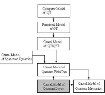
The attempt to construct a local causal model of quantum theory, including QFT resulted in 22
several refinement steps of the model (see Fig.1). At one point, it was recognized that a causal model 23
of the dynamics of QT/QFT should better be based on a causal model of the dynamics of spacetime. 24
Thus, a causal model of the dynamics of spacetime has been developed with these major goals: (1) 25
as much as possible, be compatible with general relativity theory (GRT) and (2) should match the 26
main features of the evolving model of QT/QFT. The causal model of spacetime dynamics is described 27
in [4]. Because the model of spacetime dynamics is a major prerequisite of the work described in 28
the present paper, a short description is also given in Section 4. In Section 5, the model of spacetime 29
dynamics is applied to quantum fields and quantum objects. A bottom-up approach is taken here to a 30
description of the causal model of QT/QFT dynamics. First, we describe how the model of spacetime 31
dynamics is applied to quantum fields (Section 6), and we then examine how QFT processes result in 32
the emergence of elementary particles (Section 7). Quantum loops and quantum loop processes form 33
the primary topic of this article, and play a major role in the emergence of quantum objects. After a 34
description of the model for the establishment of quantum objects, Section 8 presents a discussion 35
of quantum mechanics in terms of the model described in Section 7. In this model, in addition to 36
generating quantum objects, quantum loops evaporate two types of "field": (i) the gravitational field 37
(i.e., space curvature changes); and (ii) the Schrödinger field. The latter represents the wave function in 38
the interpretation similar to the de Broglie-Bohm theory. The model of quantum mechanics presented 39
in Section 8 therefore has some commonalities with the de Broglie-Bohm theory. 40
Figure 1.Refinement steps towards the causal model of quantum loops.
The author’s work on models of QT/QFT and spacetime dynamics has been guided by three 41
principles for models of physics theories, and the author has become increasingly convinced of these: 42
1. Causal models- the perception that it takes a causal model to explain the outcome of a physics 43
experiment, and a complete causal model to explain the experimental results for a theory as far 44
as possible. 45
2. Localcausal models - not relying on (spooky) actions at a distance. 46
3. Discretenessof the essential parameters - the assumption that there exists a minimal size and 47
granularity for the essential parameters of the theory. 48
Note that the specification of a model in the form of a local causal model is not just another style of 49
description language. The description language used in this article is a consequence of very rigid 50
requirements with respect to the required or allowed contents of the specification of a local causal 51
model. This is described in more detail in Sections 2 and 3. Adherence to the three requirements of 52
a local causal model, support for the discreteness of the essential model parameters and the need to 53
describe nonlinear dynamics have resulted in a style of writing that may be considered by the reader 54
to be not quite conformal with the style in which professional physics articles are typically written. 55
2. Causal Models 56
The formal definition of a (local) causal model has been published in various preceding papers 57
from the author. It is here repeated because it is important to the subject of this paper and because an 58
extended and refined treatment oflocalcausal models is appropriate (see Section 3). 59
Definition 1. The specification of a causal model of a theory of physics consists of (1) the specification of the
60
system state, (2) the specification of the laws of physics that define the possible state transitions when applied to
61
the system state, and (3) the assumption of a “physics engine.”
62
2.0.1. The physics engine. 63
The physics engine represents the overall causal semantics of causal models. It acts upon the state 64
of the physical system. The physics engine continuously determines new states in uniform time steps. 65
For the formal definition of a causal model of a physical theory, a continuous repeated invocation of 66
the physics engine is assumed to realize the progression of the system state. 67
68
physics engine(S,∆t):={
69
DO UNT IL(nonContinueState(S)){
70
} 72
} 73
2.0.2. The system state 74
The system state defines the components, objects and parameters of the theory of physics that can 75
be referenced and manipulated by the causal model. In contrast to the physics engine, the structure 76
and content of the system state are specific for the causal model that is being specified. Therefore, the 77
following is only an example of a possible system state specification. 78
79
systemstate:={spacepoint...}
80
spacepoint:={x1,x2,x3,ψ}
81
ψ:={stateParameter1, ...,stateParametern} 82
83
2.0.3. The laws of physics. 84
The refinement of the statement 85
S←applyLawsO f Physics(S,∆t); defines how an "in" state s evolves into an "out" state s. 86
L1:= IF c1(s)THEN s← f1(s); 87
L2:= IF c2(s)THEN s← f2(s);
88
... 89
Ln := IF cn(s)THEN s← fn(s); 90
The "in" conditionsci(s)specify the applicability of the state transition function fi(s)in basic formal 91
(e.g., mathematical) terms or refer to complex conditions that then have to be refined within the formal 92
definition. 93
The state transition function fi(s) specifies the update of the state s in basic formal (e.g., 94
mathematical) terms or refers to complex functions that then have to be refined within the formal 95
definition. 96
The set of lawsL1, ...,Lnhas to be complete, consistent and conforming to reality (see [3] for more 97
details). 98
In addition to the above-described basic forms of specification of the laws of physics byLn := 99
IF cn(s)THEN s← fn(s), other forms are also imaginable and sometimes used in this article. (This 100
article does not contain a proper definition of the used causal model specification language. The 101
language used is assumed to be largely self-explanatory.) 102
3.LocalCausal Models 103
A local causal model is a special type of causal model. The subject locality and local causal model 104
concern both, the system state and the laws of physics. 105
3.0.1. Spatial causal model 106
A causal model of a theory of physics is called aspatialcausal model if (1) the system state 107
contains a component that represents a space, and (2) all other components of the system state can 108
be mapped to the space. Many textbooks on physics (mostly in the context of relativity theory) and 109
mathematics define the essential features of a "space". For the purpose of the present article, a more 110
detailed discussion is not required. For the purpose of this article and the subject locality, it is sufficient 111
to request that the space (assumed with a spatial model) supports the notions of position, distance and 112
3.0.2. Local causal model. 114
The definition of a local causal model presupposes a spatially causal model (see above). A 115
(spatially) causal model is understood to be a local model if changes in the state of the system 116
depend on the local state only and affect the local state only. The local state changes can propagate to 117
neighboring locations. The propagation of the state changes to distant locations; however, they must 118
always be accomplished through a series of state changes to neighboring locations. Special relativity 119
requests that the series of state changes does not occur with a speed that is faster than the speed of 120
light. This requirement is not considered essential for a local causal model. 121
Based on the formal model definition of a causal model, a formal definition of locality can be 122
given. A physical theory and a related spatially causal model are given. 123
Definition 2. A causal model is called a local causal model if each of the laws Liapplies to no more than a single 124
position and/or to the neighborhood of this position.
125
The position reference can be explicit or implicit by reference to a state component that has a 126
well-defined position in space. 127
3.0.3. Local spatial specifications 128
If the causal model includes a model of spacetime dynamics (such as the model described in 129
Section 4), spatial specifications in the system state must not refer to globally (i.e., non-locally) arranged 130
position, distance and direction specifications. This requirement, which is sometimes referred to as 131
"background independence", prohibits references in terms of globally defined coordinate systems. An 132
example where this requirement applies is Definition 4 in Section 4 containing direction specifications. 133
3.0.4. Physical Objects. 134
Definition 2 notes a relatively strong type of locality that may be called "space-point locality". 135
Most physics theories and models of physics theories contain spatially extended objects (e.g., particles, 136
nuclei, stars, galaxies), with state components and attributes (such as mass, energy, momentum) that 137
apply to the object as a whole. Causal model references to the complete space of a spatially extended 138
object or to a property of the complete object are considered to violate locality. The construction of 139
alocalcausal model may not be feasible. The space point locality and the feasibility of a local causal 140
model may be regained, if it is possible to provide a model of the emergence of the object, in particular 141
the emergence of object-global components and attributes. For example, in [5], the emergence of a 142
quantum object is described as a collective behavioral process. 143
Proposition 1. Local causal models that include objects with (object-) global components and attributes are
144
feasible only, if it is possible to show a model of the emergence of the (object-) global components and attributes.
145
The emergence of the object-global components and attributes is accompanied by the emergence 146
of the object. (In general, it is possible to equate the emergence of the object-global components 147
and attributes with the emergence of the object). Two typical ways/processes for the emergence of 148
object-global components and attributes are 149
1. Aggregation of subcomponent attributes (example: aggregation of the mass of a physical object) 150
2. Synchronization of subcomponents attributes (examples: paths, velocity, momentum, angular 151
momentum of a composite quantum object) 152
In Section 7, the model of the emergence of a quantum object is described as a nonlinear collective 153
3.0.5. Global/local laws of physics. 155
The provision of a local causal model may also be impeded by the existence of (object-) global laws 156
of physics. Global laws of physics are laws that apply to a complete object. From the definition of a 157
causal model given in Section 2, this means that the respective law of physicsLirefers to some (object-) 158
global components or attributes. Examples of global laws of physics are all kinds of conservation laws 159
(e.g., energy conservation, momentum conservation), and the second law of thermodynamics (i.e., 160
entropy law). In addition, the laws of quantum theory represent object-global laws, because the wave 161
function may apply to a collection of particles.1The existence of global laws within a theory of physics 162
must not necessarily mean the non-feasibility of a local causal model, because the causal model may 163
not include the global law within the relevant listL1,L2, ...Lnof the causal model. For example, the 164
entropy law should not appear within a causal model. Neither should theglobalconservation laws 165
appear in a causal model. The global conservation laws have to be broken down to (space-point) local 166
conservation laws (which means the local laws have to obey the well-known symmetry requirements). 167
Even for global laws of physics that cannot be broken down to local laws, there may be ways to 168
construct a local causal model. Because (as described above) a global law implies that there must be 169
global object components and attributes, the feasibility of a local causal model may be regained, if it is 170
possible to provide a model of the emergence of the object, in particular the emergence of object-global 171
components and attributes. 172
4. The Local Causal Model of Spacetime Dynamics 173
4.1. The elementary structure of space(-time)
174
In the model described in this article, the system state consists of the space, fields and quantum 175
objects. (Time is not considered part of the system state (see below "The space-time relationship")). 176
Definition 3. System state :=
177
Space,
178
Fields,
179
Quantum objects;
180
Definition 4. Space := { spacepoint ...};
181
spacepoint := {ψ,gravitationspec,connections };
182
connections := { connection1, ...,connectionn}; 183
connection := { neighborspacepoint,direction };
184
gravitationspec := { gravdynamic,direction,gravstrength };
185
186
ψrepresents the contents of space in the form of fields and quantum objects (see Section 5 for more
187
details). According to Section 3, direction has to be a local parameter. As described in Section 3 "Local 188
spatial specifications", to enable alocalcausal model, the direction specification of the connection must 189
be given in terms of space-point-local parameters. In Section 6.4, a possible direction specification 190
schema is described. 191
4.2. The space-time relationship
192
In GRT and SRT, space and time are said to be integrated into spacetime. From a mathematical 193
perspective, the integration of space and time is reflected in the use of vectors, matrices and tensors 194
1 The object global nature of the wave functionψrepresents the root of the apparent non-feasibility of a local causal model of
that combine the dimensions of space with that of time. The integration is also reflected in the laws of 195
physics, where space and time (and their derivatives) are jointly transformed. As described above, in 196
the causal model chosen here, space and time are strictly separated. Since this model also aims for 197
maximal compatibility with GRT, the question arises of how this compatibility can be achieved with a 198
model in which space and time are fundamentally (initially) not integrated. In the concept underlying 199
the causal model of spacetime dynamics, space-time integration does not apply to space and time in 200
general, as in SRT and GRT; instead, 201
space-time integration only applies to physical processes executed in space and time.
202
This implies the following: 203
Proposition 2. The measure and metric for space and time can only be defined jointly for both space and time,
204
and only with reference to a specific process that produces a specific rate of spatial change (i.e. length) within a
205
specific time interval.
206
The physical process that is best suited for this joint definition of the measure for space and time 207
is the movement of light, under the assumption that the speed of light is a constant. 208
Proposition 3. The execution speed of physical processes in terms of changes in length in relation to the
209
execution time is invariant.
210
For example, if a clock rate (i.e., the proper time) changes, this is always accompanied by a length 211
dilation in the space where the process is executed. 212
The major physical expressions of curved spacetime are length and time dilations.2 "Time dilation" 213
essentially means a dilation of the speed by which physical processes, such as clocks, run. 214
As a special case of Proposition 2 and 3: 215
Proposition 4. Length and time dilations are interrelated and occur only in combination.
216
Propositions 2 and 3 are essential in the more detailed model of spacetime dynamics described 217
below. The above basic propositions with respect to the space-time relationship lead to the following 218
propositions concerning the elementary structure of spacetime: 219
Proposition 5. The state update time interval, suti is a constant of nature.
220
Proposition 6. The distance between two neighboring space points, lconnection, is a constant of nature. This is 221
the distance through which light moves during a suti.
222
(In Euclidean geometry, it is difficult to imagine that all space point connections have the same 223
length if the connections are not restricted to orthogonal directions.) 224
In a model that assumes a constant speed of light, c, it follows from Propositions 5 and 6 that: 225
Proposition 7. During a state update time interval, suti, light moves a constant distance, namely the distance
226
lsuti =lconnection =suti·c 227
The proposed model of spacetime dynamics assumes that all distances and lengths in space 228
are composed of the elementary length units,lsuti. Likewise, all time intervals are multiples ofsuti. 229
Lengths and distances are defined only between two space points and only with reference to the speed 230
of light, c. 231
Proposition 8. The distance between two space points, sp1and sp2is given by the number of spacepoints,
232
nsp(sp1,sp2)through which light passes when moving from sp1to sp2multiplied by the elementary length
233
unit, lsuti(= lconnection). 234
distance(sp1,sp2) =nsp(sp1,sp2)·lsuti. 235
The above propositions result in a model of spacetime in which the speed of light is a constant. 236
However, due to Proposition 5, it is hard to avoid curved space. This does not present a problem, since 237
curved spacetime is not undesirable in a spacetime model aiming for compatibility with GRT. The 238
remaining problem is that of how to achieve GRT-compatible space curvature. Spacetime curvature 239
due to time dilation (as predicted by GRT) also needs to be supported. The solutions offered by 240
Propositions 3-7 are that (i) the process of space emergence/expansion (Section 4) results in length 241
dilations through the suitable arrangement of space points and that (ii) length dilations cause clock 242
rate dilations for processes running at space positions with dilated lengths. 243
The formal expression of point (i) is: 244
Proposition 9. Lengths within the gravitational field are dilated by the factor F1.
245
The precise equation for the factor,F1, such that it is in accordance with GRT is given below. For
246
the model described in this article, the revised formulation of Proposition 4 is: 247
Proposition 10. Physical processes run faster or slower depending on the length dilation at the position in
248
which the respective physical process is executed.
249
Proposition 9 may be viewed as a refinement of Proposition 3 above where the dilation of the 250
clock rate concerns physical processes rather than the structure of spacetime. The major process 251
that demonstrates the fixed relationship between the length dilation and the rate of change of the 252
process is the propagation of light. This (simple) process is used as a measure for the change rate 253
of other processes by setting the speed of light to be a constant, c. The next classes of processes in 254
which the rate of change depends on the length dilation in precisely the same proportions as in the 255
propagation of light are clocks in differing realisations. In summary, there is no direct reflection of time 256
dilation as an attribute of spacetime in the model of spacetime dynamics. Clock rate dilation (rather 257
than time dilation) arises as a property of processes running within space. The clock rate dilation 258
factor can be derived from the length dilationfactor,F1of the space points at which the respective 259
process is currently being executed. Thus, in the model of spacetime dynamics, two levels of time are 260
distinguished, although these are seen as a single entity in GRT/SRT: 261
1. At the basic level, the progression of time is determined by the uniform state update time interval, 262
suti. Simultaneity is assumed for all state changes occurring within the same state update cycle. 263
2. Differing clock rates, proper times, and the relativity of simultaneity are not associated with the 264
basic overall spacetime (level 1), but instead are associated with physical processes running in 265
space. 266
In terms of space, two levels can also be distinguished, although these are two levels of consideration: 267
• At the abstract level (the mathematical level), the space consists of a set of interconnected space 268
points. The issue of whether or not the totality of the interconnected space points represents a 269
Euclidean space or a specific topology (e.g., a Riemann manifold) is left open. 270
• At the physical level (the essential level), physical meaning is assigned to the components of 271
the space point and its connections. In particular, the length of the connections is no longer a 272
geometrical property, but specifiesonlythe∆length through which light moves during the state 273
Thus, the integration of space and time into spacetime is established in the model of spacetime 275
dynamics by the physical meaning assigned to the components of the space points and their 276
connections. 277
4.2.1. The length dilation factorF1.
278
In GRT, the curvature specification (i.e., the curvature tensor), contains a time-related component in addition to the three space-related components. As an example of the impact of the time factor, the gravitational redshift is explained as the consequence of the time factor in the spacetime curvature (see, for example, [6], page 231). With a Schwarzschild metric
∆s2=−(1−2GM c2r )(c∆t)
2+ (∆x)2+ (∆y)2+ (∆z)2 (1)
This means that a clock at position (x, y, z) would run slower than a clock that is not affected by a gravitational field by a factor
F1= r
1−2GM
c2r (2)
A standard clock at some point A of low potential (for example, at the surface of the earth) would 279
run slower than the same clock at a point B with higher potential (for example, in a GPS satellite). 280
Proposition 8 states that not only are the clock rates of clocks within a gravitational field dilated by the 281
factorF1, but that this dilation also applies to lengths. (As a supporting argument, only in this way can 282
the proposition of the constant speed of light be maintained.) Proposition 9 also means that length 283
dilation is the primary effect, and that the clock rate dilation for clocks residing in the length-dilated 284
space is a consequence of the length dilation. 285
4.2.2. Energy dilation with objects moving in curved space 286
Proposition 11. When an object (e.g. a particle) moves from one space point, sp1, to another, sp2the energy of
287
the object decreases or increases as a function of the difference in the gravstrength of the two space points.
288
The energy difference associated withsp1andsp2is usually called the (difference in) potential
289
energy of the positions ofsp1andsp2. Thegravstrengthand thus the energy, increases or decreases 290
and has a direction, which is towards the source(s) of the gravitation. The basic types of energy that 291
are affected by the increase or decrease in the positional energy are the kinetic energy and the wave 292
energy (i.e., the wave frequency and wavelength). 293
4.3. The dynamics of space emergence and space changes
294
With the proposed model, it is assumed that all the dynamics of space changes, including the 295
emergence of space, starting from a minimal source and proceeding through the successive addition of 296
new surface layers of space points. The number of space points at the surface layer increases with each 297
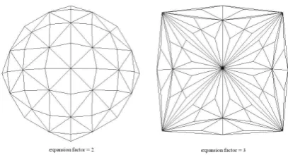
new surface layer. The space expansion factor (implied by the space expansion algorithm) determines 298
the increase of the number of space points with the new surface layer. Fig.2shows examples of space 299
surface layers with different expansion factors (2 or 3).3. The space expansion algorithm must achieve 300
compatibility with GRT. This affects two items: 301
1. The expansion factor that determines the growth of the number of space points at the surface 302
layers must be such that Eq.2is satisfied (which means that a Schwarzschild metric arises). 303
3 Remember that we are dealing with curved space and that this cannot be adequately represented in the 2-dimensional
Figure 2.Surface of small space objects with radius=3·lsuti.
2. The gravstrengthin Definition 4 that specifies the strength of the gravitational fieldψG must 304
decrease with the increasing distance from the source of the gravitation (see parameter r in Eq.2). 305
If multiple sources are in the process of aggregation (see below), the strength of the gravitational 306
field has to accumulate accordingly. 307
The process of space state progression consists of the repeated application of Spread-out/Bundle
308
operations to all space points that are identified by 309
gravdynamic6=0 (see Definition 4). 310
Definition 5. Space-state-progression(space sp):={
311
Spread-out: FOR ( ALL spacepoints sp.point[i]){
312
IF ( sp.point[i].gravdynamic6=0) {
313
generate-OUT-points-from( sp.point[i]);
314
}
315
Bundle: FOR ( ALL new spacepoints sp.point[j]){
316
accumulate-inconnections ( sp.point[j]);
317
}
318
}
319
The expression "generate-OUT-points-from( )" generates new space points (including the necessary 320
connections) for all space points that are currently with this attribution: gravdynamic 6=0. At least 321
one new space point is generated. Whether further space points and connections emerge depend on 322
the gravitational strength and on the more detailed algorithm for the emergence of space changes. 323
The gravitational strength is reduced as a function of the increasing distance from the gravitational 324
source(s). The new space points are temporarily marked as NEW in the "Bundle" step, in which the 325
gravitational strengths are accumulated for all connections to the new space point. The function 326
"generate-OUT-points-from" can be expressed by the following specification. 327
Definition 6. generate-OUT-points-from ( sp.point ) := {
328
point0←generate-primary-outpoint(sp.point);
329
add. points←generate-additional-outpoints(sp.point);
330
supplement-connections();
331
}
332
4.3.1. Aggregation of space changes from multiple sources. 333
The assumption that all space change dynamics starts from minimal sources implies that the space 334
changes originating from multiple sources, typically, will soon start to overlap and will accumulate. 335
• Phase 1: The space changes from the individual sources propagate by the addition of spherical 337
surface layers as described above. The changed space object represents a Schwarzschild metric 338
and Eq.2is satisfied. 339
• Phase 2: The space changes overlap and have to be accumulated. The accumulated space object 340
does not represent a Schwarzschild metric and Eq.2is not applicable. 341
• Phase 3: At a suitable distance from the gravitational sources, the gravitation may be handled as 342
if there was a single source with the mass equal to the sum of the multiple sources of masses 343
located at the centre of masses. Eq.2is applicable again. 344
Further details on the subject of Section 4 can be found in [7] and [4]. 345
4.3.2. Sources of space change dynamics. 346
In [7] and [4], the sources of space change dynamics are described as quantum objects. In the 347
present article, the model of spacetime dynamics is also applied to the dynamics of quantum objects 348
and quantum fields. This leads to a refinement of the model in which the elementary processes within 349
the quantum objects are already sources of space change dynamics (see Section 6.1). 350
5. Application of the Model of Spacetime Dynamics to QT/QFT 351
The local causal model of spacetime dynamics described in [7] and [4] and summarized in Section 352
4 has been developed with the goal of providing a basis for a local causal model of QT/QFT. The 353
application of the model to quantum theory and quantum field theory is described in the following: 354
5.1. The space contents
355
Definition 3 defines the system state of the local causal model of spacetime dynamics as consisting 356
of space, fields and quantum objects. Fields and quantum objects may be viewed as the contents of 357
space. In Definition 4, the space point is defined as containing the componentψ.ψis said to represent
358
the point-local content of the space. Application of the model of spacetime dynamics to QT/QFT 359
requires (1) a more detailed specification of the space contentsψand (2) the specification of the model
360
of the dynamics of the spacecontents. 361
5.1.1. The space point componentψ
362
may represent different types of space contents, that is, different types of fields and of particles. 363
The possible types of ψcontain the field types known from QFT (e.g., the electromagnetic field),
364
the gravitational fieldψG4and the "Schrödinger field"ψSthat represents the wave function. 5 The 365
association ofψto the space point is not a static association. The space point content may move and
366
spread out to neighboring space points. Also, theψof a common type may form collections such as
367
fields, particles and composite quantum objects. Such collections ofψmay emerge to physical objects
368
(i.e., quantum objects) that propagate as an entity with special object-global attributes. 369
The more detailed components ofψdepend on the field type. A fairly general set of components and
370
attributes is 371
Definition 7. ψ:={
372
dynamics attributes,
373
spin type, spin value,
374
charge type, charge value,
375
4 In Definition 4, the gravitational fieldψ
Gis represented by thegravitationspecattribute.
5 The relation between the Schrödinger fieldψ
direction
376
}
377
dynamics attributes := { amplitude, frequency }
378
5.1.2. Fields 379
are the simplest type ofψcollections
380
f ield:={spacepoint1.ψ,spacepoint2.ψ, ...}.
381
All the space points belonging to the field have the same field type associated. In contrast to quantum 382
objects, there are no object-global attributes associated with the field. This makes the fields a suitable 383
base for the specification of a (space point) local causal model of QT/QFT. 384
5.1.3. A quantum object 385
is defined as consisting of a collection of 1 to n particles (see [8]). This means that a quantum 386
object is either an elementary particle or a composite quantum object. 387
Definition 8. quantumobject:={
388
globalquantumobjectattributesΩ;
389
particle1, 390
...
391
particlen; 392
}
393
The collection of particles is supplemented by global attributesΩ1,Ω2, ...Ωj,.
394
The elementary particle encompasses the ψ-components of a set of spacepoints and
395
global particleattributesΘ1,Θ2, ...Θj,.
396
Definition 9. particle:={
397
global particleattributesΘ;
398
spacepoint1,spacepoint2...}.
399
}
400
Examples of global attributes are Ωmass,Ωcharge and Ωspin. As described in Section 3, the 401
occurrence of global attributes in alocalcausal model may disturb the (space point) locality of the 402
model, if it is not possible to show the emergence of the global attribute from (space point) local 403
parameters. 404
5.2. Space contents dynamics
405
The model of the dynamics of space contents (quantum fields and quantum objects) is formulated 406
using a bottom-up approach. The basis of the causal model of QT/QFT is the local causal model of 407
quantum fields (Section 6), an extension of the local causal model of spacetime dynamics described in 408
[7] and [4] and summarised in Section 4. Quantum objects emerge from quantum fields. In this way, the 409
model distinguishes the emergence of elementary particles and the dynamics of composite quantum 410
objects. Elementary particles emerge directly from quantum fields in a collective behaviour process 411
called a quantum loop (Section 7). The dynamics of the complete quantum mechanics, including 412
6. Quantum Field Dynamics 414
6.1. Energy-carrying space points - the sources of quantum field dynamics and spacetime dynamics
415
In [7] and [4] and in Section 4.3, quantum objects are denoted as the sources of spacetime dynamics. 416
With the application of the model of spacetime dynamics to QT/QFT, quantum objects remain a source 417
of spacetime dynamics; however, the model is refined to include, in addition, specific space points as 418
the source of spacetime dynamics and as the sources of quantum field dynamics. The space points 419
that are sources of spacetime dynamics may be calledenergy-carrying space points. The contents of 420
energy-carrying space points propagate through space. In the formal specification of the QT/QFT 421
model, energy-carrying space points contain non-empty dynamics attributes as part of the field 422
contentsψ(see Definition 7). A space pointspiis never a permanent source of quantum field dynamics. 423
After the propagation of the contents ofspihas taken place, the dynamics attributes are reset to zero. 424
In addition to the dynamics attributes (indicating that the space point is an actual source of 425
quantum field dynamics), the propagation direction is specified as an additional attribute. According 426
to Definition 7, the fields represented byψmay have different spin values. In the model described here,
427
fields may have spin 1/2 (a fermionic field) or spin 1 (a bosonic field). In addition to the classical field 428
types, two (secondary) types of fields are generated in the dynamics of energy-carrying space points: 429
1. Gravitational fields,ψG: The dynamics of space changes (i.e., of gravitation) was the starting
430
point for the causal model of quantum field dynamics. The integrated model of spacetime and 431
quantum field dynamics considers gravitation as a special type of field. 432
2. Schrödinger-fields, -ψS: The wave function of quantum mechanics requires a representation at
433
the space (point) content and a causal model of its dynamics. In the model described here, this 434
"field" is called the "Schrödinger-field" -ψS.
435
These two types of field are considered to be secondary fields, since they do not carry energy, meaning 436
that: (i) the creation of these types of fields due to the propagation of energy-carrying space points 437
does not reduce the energy of the source; and (ii) the fieldsψGandψSare not capable of interacting 438
with other quantum fields and quantum objects by exchanging energy. Unlike primary fields, the 439
propagation of secondary fields does not need to preserve the direction of momentum. This enables 440
the expansion of these fields to create/cover an ever-growing volume of space. 441
6.2. Quantum fields are waves
442
Waves and fields are the basic constituents of quantum field theory. Since we are dealing here 443
with the lowest level of space granularity, it is difficult to imagine the application of the classical model 444
of waves to the model of quantum field dynamics. Nevertheless, there are a number of properties 445
that are known from the physics of waves that also appear to be useful in the model of quantum field 446
dynamics presented here. A very short introduction to waves in physics is therefore given in the 447
following. The description below is derived from [9] and to a larger extent from [10]. 448
The standard formulation of the "wave equation", that is, the equation of motion for waves, is (see, for example [9])
(1 v2
∂2 ∂t2− 5
2)
ψ(x,t) =0 (3)
Depending on the particular context, this equation may be varied or extended by setting the right-hand side not equal to zero. For example, in [10], two classes of waves, Class 0 and Class 1, are distinguished: Class 0:
d2ψ/dt2−cw2d2ψ/dx2=0. (4)
Class 1:
For the mapping of QFT to the causal model of QT/QFT, the way in which the energy of a wave is 449
reflected in the wave equations is important. In [10], the quantum waves are described by a motion 450
formula 451
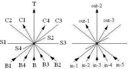
Z(x,t) =Z0+Acos(2π[νt−x/λ])
where A is the amplitude,λis the wavelength andν is the frequency. In quantum mechanics, the
amplitude A is restricted to discrete values. The equation of motion requires that the frequency and wavelength be related toνmin(appearing in Eq.6) by the formula
E2= (hν)2= (hc/λ)2+ (hνmin)2 (6) This looks like a Pythagorean relation ( i.e.,c2=a2+b2). Another Pythagorean relation, well-known 452
in relativity theory, describes the relation between total energy E, the kinetic energyp·mand the mass 453
energymc2by
454
E2= (pc)2+ (mc2)2
455
This suggests the following equation for the total energy, the kinetic energy and the mass energy: 456
E=hν;pc=hc/λ;mc2=hνmin. 457
A (simple) wave of a given frequency and wavelength is made up of n quanta. The allowed values of 458
the amplitude A are proportional to√n. For bosons, the allowed values of the energy are 459
E= (n+1/2)hν, where n = 0,1,2,3,4,. . . .
460
For fermions the allowed values are 461
E= (n−1/2)hν, where n = 0 or 1.
462
In addition to the above considerations, which relate to the propagation of a single wave, the physics 463
of interacting waves offers another basis for a causal model of quantum field dynamics. In [10], an 464
example of the interaction of quantum fields is described by three equations of motion in which the 465
interacting waves occur on the right-hand side: 466
d2A/dt2−c2d2A/dx2=yBC. 467
d2B/dt2−c2d2B/dx2=yAC. 468
d2C/dt2−c2d2C/dx2= (2πν
min)2C+yAB. 469
Depending on the specific attributes of the interacting waves, other expressions describing the results 470
of this interaction are also possible, and the example given in [10] is 471
d2S/dt2−c2d2S/dx2= (2πνmin)2(m2S[S−S0] +y2SZ2). 472
d2Z/dt2−c2d2Z/dx2= (2πν
min)2y2S2Z. 473
Further rules for the determination of the results of interacting fields are given in QFT, in terms of the 474
Feynman rules for particle scattering. 475
Although it does not appear to be reasonable to apply the classical model of waves in its entirety 476
to the causal model of quantum field dynamics, the following items are taken over and mapped to this 477
model: 478
• The energy of an energy-carrying space point is proportional to the amplitude and frequency 479
parameters. 480
• The allowed values of the amplitude A are proportional to√n
481
• For bosonic energy-carrying space points, the allowed values of the energy areE= (n+1/2)hν,
482
where n = 0,1,2,3,4,. . . . 483
• For fermionic energy-carrying space points, the allowed values are: 484
E= (n−1/2)hν, where n = 0 or 1.
485
• There may be a minimal frequencyνmin.
486
• Eq.6may also apply to the propagation of energy-carrying space points. 487
6.3. The Interaction Operatorχ
488
In the model of the propagation of space contents (fields and quantum objects), the space point 489
typical space point, with 14 connections that span the whole neighbourhood space. In the proposed 491
causal model of QT/QFT, all space point connections may be utilised for the propagation of fields 492
(i.e., gravitational, fermionic, bosonic, Schrödinger field). This enables support for the concurrent 493
propagation of the different field types. All space point connections are utilised for the propagation 494
of the gravitational field and the Schrödinger field, and all connections that are not in-connections 495
become out-connections. In the propagation of fermionic and bosonic fields, the direction has to be 496
preserved in the form of geodesic paths. This includes the possibility of the creation and annihilation 497
of field types according to the rules of QFT (e.g. Feynman rules). Unlike in standard QFT, multiple 498
bosonic field connections are possible. If more than one bosonic in-connection occurs (dynamically) at 499
a space point, the bosonic in-connections are accumulated and treated like a single in-connection. A 500
bosonic out-connection may be distributed to multiple out-connections. 501
Figure 3.Example of the distribution of connections of a space point.
The propagation of quantum fields through space is concentrated in the interaction operatorχ.
502
χ(sp)corresponds to combinations of creation and annihilation operators in QFT, and applies to a
503
space point sp, including its dynamically assigned in-connection and out-connections. For a given 504
space point, sp, it determines the out-connections and the new state (including contents) of the space 505
points that are targets of the out-connections as a function of the content of sp. The overall field state 506
progression can be expressed as: 507
Field-state-progression(space):={
508
FOR ( ALLspacepoints sp[i]){
509
IF (sp[i].gravdynamic6=0 ORsp[i].ψ.dynamicsattributes6=0)
510
applyχ(sp);
511
} } 512
Definition 10. applyχ(sp):= {
513
Spread-out:
514
determine-gravitational-out-connections(sp);
515
distribute-gravitation(sp);
516
distribute-ψS(sp); 517
IF (sp.ψ.dynamicsattributes6=0){
518
IF (sp.ψ.spintype=1/2)distribute-fermion(sp);
519
else distribute-boson(sp);
520
}
521
Bundle:
522
FOR ( ALL spacepoints sp[i]WITH inconnections) {
523
bundle-gravitational-inconnections( sp[i]);
524
bundle-ψS-inconnections( sp[i]); 525
bundle-ψ-inconnections( sp[i]);
526
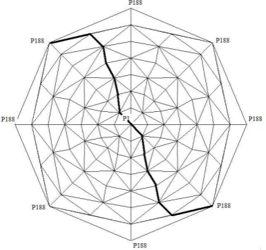
set-dynamics-attributes( sp[i]);
}
528
}
529
Thus, the application ofχ(sp)consists essentially of a combination ofSpread-outandBundle,
530
whereSpread-outdetermines the out-connections of sp andBundlebundles all in-connections of those 531
space points that have them (resulting fromSpread-out). For the gravitational fieldψgthe combination 532
ofdistribute-gravitation()andbundle-gravitational-inconnectionsresults in the propagation of space 533
(curvature) changes as described in Section 4.3. The Schrödinger-fieldψSis assumed to propagate in a 534
similar way to the gravitational field, except that the Schrödinger equation in Eq.8must be obeyed. 535
The combination of { distribute-fermion() and distribute-boson() } andbundle-ψ-inconnections()
536
is more complicated, since the rules of QFT (e.g. the Feynman rules) must be satisfied. This means, for 537
example, that distribute-fermion(sp) must not result in two fermionic out-connections of the same type 538
and charge. In addition, in bothSpread-outandBundle, the energy and momentum must be preserved. 539
The detailed determination of the momentum and energy of the out-connections is also derived from 540
QFT, although with significant adaptations due to the characteristics of the causal model. The major 541
differences from standard QFT are as follows: 542
• The model of quantum field dynamics described here applies to energy-carrying space points, 543
while the QFT rules for the calculation of scattering matrix amplitudes apply to (virtual) particles. 544
• Since this is a causal model, the amplitude associated with a propagation path must be an 545
explicit system state parameter that has a non-probabilistic meaning. In the proposed model, the 546
amplitude of an energy-carrying path is a measure of the energy of the energy-carrying space 547
point (as opposed to a probability amplitude). 548
• There is no relativity of time progression (at the level of quantum field dynamics). 549
• Since the model is alocalcausal model,χ(sp)must depend only on space point-local parameters.
550
This affects the parameter "mass", which occurs frequently in standard QFT for calculations of 551
scattering matrices. Another implication is that the specification of spatial directions must be in 552
terms of space point-local parameters (see below Section 6.4). 553
• Since a space point has only a small, discrete number of connections to neighbouring space points, 554
only a small set of possible directions (or even a single definite direction) must be determined, 555
where QFT applies integrals that span the total space. 556
• Distances between vertices have a fixed length (i.e,. the length of space point connections are 557
constant=Lconnection, see Section 4.1). 558
• The possible energy and momentum values are quantised (i.e., discrete values with a non-zero 559
minimum value). 560
6.4. The local space-point specification of directions
561
The laws of physics require conservation of momentum when the field contentsψof fermionic
562
or bosonic fields propagate from the in-connection(s) of a space point to the out-connection(s). 563
Conservation of momentum means (besides conservation of the amount) conservation of the direction 564
of the propagation. That is, the direction of the out-connection must be equal to the direction of the 565
in-connection. For example, in Fig.3the direction of in-3 is equal to that of out-2. The requirement 566
of direction conservation is a trivial requirement with non-curved (e.g. Euclidean) space with global 567
direction specification in terms of a globally agreed coordinate system. With alocalcausal model 568
according to Section 3 and curved discrete space, the implementation of the requirement is less 569
trivial. As described in Section 3 "Local spatial specifications", to enable alocalcausal model, the 570
direction specification of the connection must be given in terms of space-point-local parameters and 571
the algorithm for the determination of out-connections must use only the local direction specification. 572
A direction specification scheme that satisfies this requirement is (roughly) described in the following. 573
To simplify the description, let us assume that the typical space point has 14 connections with the 574
• B: The connection from the direction of the source (e.g. in-3 in Fig.3) 576
• T: The connection from the direction away from the source (e.g. out-2 in Fig.3) 577
• S1, S2, S3, S4: The connections that are orthogonal to B and T. 578
The connectionsSiare those connections between space points that have an equal distance from 579
the gravitational source. In the model of the emergence of space described in Section 4, the 580
emergence of space continuously develops surfaces such as the ones shown in Fig.2that consist 581
ofSiconnections ("S" stands for surface). 582
• B1, B2, B3, B4 The connections between B and S1, S2, S3, S4 (e.g., in-1, in-2, in-4, in-5 in Fig.3) 583
• C1, C2, C3, C4 The connections between T and S1, S2, S3, S4 (e.g., out-1, out-3 in Fig.3) 584
This direction specification scheme assumes that for each connection/direction an opposite 585
connection/direction exists. If the set of connections is {B, T, S1, S2, S3, S4, B1, B2, B3, B4, C1, 586
C2, C3, C4 }, the corresponding opposite connections are opposite( {B, T, S1, S2, S3, S4, B1, B2, B3, B4, 587
C1, C2, C3, C4 }→
588
{T, B, S3, S4, S1, S2, C3, C4, C1, C2, B3, B4, B1, B2, } 589
Based on the above direction specification scheme and the existence of theopposite()operator, it is 590
possible to determine the out-connection for a given in-connection.6The successive application of the 591
scheme determines geodesic paths through discretized curved space. As a general observation, the 592
assumption of discrete entities, such as discrete geodesic paths, may result in non-smooth effects at a 593
very small scale. 594
6.4.1. Geodesics of quantum fields in the model of spacetime dynamics 595
The geodesics of energy-carrying space points are determined by (i) the structure of spacetime, 596
and (ii) the algorithm that decides which out-connection(s) correspond to the given in-connection(s). In 597
the simplest case, where a single out-connection is assigned to a single in-connection, the determination 598
of the out-connection that corresponds to a given in-connection is straightforward. As described in 599
the above space-point local specification scheme, for each possible in(out)-connection there exists 600
an opposite out(in)-connection. Notice, however, that because we are dealing with curved discrete 601
space, the "opposite" direction cannot be defined in the same way as in Euclidean space. Nor is it 602
possible to define geodesics in the way they are defined with differentiable Riemannian manifolds. In 603
a model of spacetime dynamics in curved discrete spacetime, direction conservation and geodesics 604
must be defined in terms of space point-local parameters, that is, in terms of the discrete space-point 605
connections. This may lead to geodesic paths that loop on the surface of an emerging space object (see 606
Section 7, Quantum loops). 607
7. Quantum Loops 608
Proposition 12. Quantum objects, elementary particles as well as composite quantum objects, are realized by
609
quantum loops.
610
The assumptions that (1) space dynamics (e.g., the emergence of space and the propagation of 611
space changes) starts already at the energy-carrying space points and that (2) a de facto strong space 612
curvature near the minimal sources of space dynamics already exists, enable a causal model of the 613
emergence of quantum objects. The collective behavioral process, called "quantum loop" emerges 614
when a multitude of energy-carrying space points are confined in a small volume of curved space 615
called the quantum loop shell. 616
6 The assumption of 14 space point connections and the validity of the symmetric opposite() operator (i.e., opposite(opposite(c))
7.0.1. Collective behavioral processes 617
are characterized by the (loosely) synchronized behavior of a collection of elements of equal type. 618
Prerequisites for the occurrence of collective behavior are (see, for example [5]): 619
• a multitude of elements of equal type, 620
• elements residing within a (small) volume of space such that interactions between the elements 621
are enabled, 622
• interactions between the elements that lead to synchronizations with respect to specific properties, 623
Typically, external influences can support or destroy the collective behavior and phase transitions 624
occur when the frequency and strength of the interactions increases or decreases due to collective 625
energy increase/decrease. Collective behaviour is always the result of some process with possible 626
nonlinear phase transitions to stable states. These stable states may be called "quantum equilibrium" 627
(see Section 8.4, Proposition 17 and [11] for more details on quantum equilibrium). 628
7.0.2. Major characteristics and parameters of a quantum loop. 629
Quantum loops constitute quantum objects, elementary particles and composite quantum objects. 630
In the present article, only the generation of elementary particles by quantum loops is discussed in 631
detail (the generation of composite quantum objects is briefly discussed in Section 7.5). Quantum loops 632
that form elementary particles have the following components and characteristics: 633
• The space occupied by the quantum loop containsNspspace points. Since the quantum object 634
represented by the quantum loop is generally moving, the set of space points occupied by the 635
quantum loop changes dynamically. In addition, the size of the quantum loop,Nsp, can vary 636
dynamically. 637
• Of theNspspace points belonging to the quantum loop,Necspace points are energy-carrying 638
space points (Nec < Nsp). As a consequence of the continuous interactions between the Nec 639
energy-carrying space points,Necalso changes dynamically. 640
• The set ofNecenergy-carrying space points has a major field typeψql. Due to the continuous
641
interactions between the energy-carrying space points, field types other than the major field type 642
ψqlmay temporarily occur. 643
• The total energy of the quantum loopEqlis constant (if external influences are excluded). 644
• As a result of the collective behaviour process, the energies of the energy-carrying space points 645
Eecwill become (roughly) equal toEec=Eql/Nec. 646
7.0.3. Conditions for the constitution of quantum loops. 647
For the emergence of quantum loops and, more importantly, for the stable lifetime of an established 648
quantum loop, two conditions must be satisfied: 649
1. The space within which the internal quantum loop dynamics is executed must have a curvature 650
that enforces the confinement of the energy-carrying space points within the shell. 651
2. The quantum loop dynamics (i.e., the propagation and interactions of the energy-carrying space 652
points) must preserve the energy of the total quantum loop,Eql. 653
The first condition concerns the model of spacetime, and in particular its curvature (Section 4), while 654
the second concerns the model of quantum field dynamics, and in particular the interaction operatorχ
655
(Section 6.3). 656
7.1. The gravitational fieldψGaround the sources of space dynamics 657
In Section 4, the model of the emergence of space and of the propagation of space changes is 658
described as resulting in the development of successive layers of spherical surfaces, with a strong 659
6.1 assumes that the energy-carrying space points are already deeper sources of space curvature and 661
gravitation. In this model of spacetime dynamics, space curvature is represented by two parameters: 662
1. Space curvature is represented by the density of these space points and by the arrangement of 663
the connections between them. As described in Section 6.4, energy-carrying space points follow 664
geodesic paths in space. If a geodesic path lies on a surface layer around the gravitational source 665
(i.e., if the path moves from space pointsp1tosp1, where both space points are at equal distances
666
from the source), the geodesic path continues at the surface layer, forming a "geodesic loop". 667
2. The gravitation field ψG is assigned to each space point in form of the gravitationspec (see 668
Definition 4). The variations in thegravstrengthmay be viewed as the establishment of space 669
curvature.7 670
Both effects may contribute to the confinement of the quantum loop within the quantum loop shell. 671
Scenarios can be imagined in which the collective behaviour of the energy-carrying space points results 672
in a significant proportion of them ending up in a geodesic loop. Fig. 4shows the mapping of the 673
surface of the space object shown in Fig.2to a two-dimensional flat plan, and an example of a geodesic 674
loop on that surface (the space curvature is not recognisable in both Fig.4and Fig.2). With the chosen 675
type of 2D mapping, one pole of the surface (e.g., the north pole P1) is shown at the centre, while the 676
opposite pole (e.g., the south pole, P188) appears eight times. The bold path shown in Fig.4represents 677
a simple geodesic loop around the surface, which meets the space points P1 and P188, among others.
Figure 4.2D-map of the spherical surface of the space object shown in Fig. 2.
678
We assume that of theNecenergy-carrying space points,Nloopend up in geodesic loops (possibly 679
at different surface layers). The remainingNradialpoints (Nradial =Nec−Nloop) cannot be prevented 680
from periodically leaving the scope of the (narrow) quantum loop surface, resulting in an oscillating 681
behaviour. These oscillating energy-carrying space points will leave the quantum loop only for a small 682
distance before returning to the quantum loop. The set of energy-carrying space points belonging to 683
the quantum loop have an overall vector of momentum with a specific direction (and size). The overall 684
direction is preserved during and after the formation of the quantum loop. However, theNlooplooping 685
energy-carrying space points cannot contribute to the overall direction of momentum. The looping 686
energy-carrying space points are direction-neutral. This leads to Proposition 13: 687
Proposition 13. The overall momentum (direction and amount) of the quantum loop and the momentum-related
688
energy are determined by the sum of the momenta of the oscillating energy-carrying space points. The mass
689
(energy) of the quantum object represented by the quantum loop is determined by the sum of the energies of the
690
looping energy-carrying space points.
691
Notice that the total energyEtotalof the quantum loop is not simply the sum of the momentum 692
energyp·cand the mass energymc2, but is determined by 693
Etotal = p
(pc)2+ (mc2)2.
694
7.2. QFT within the quantum loop
695
The second type of condition that must be satisfied for a quantum loop to form and remain stable 696
concerns the QFT-related details of the quantum loop internal dynamics, and in particular the details of 697
the interaction operatorχ(see Section 6.3). The essential part of the quantum loop dynamics concerns
698
the fermionic and bosonic energy-carrying space points. In each state update cycle of the process, the 699
interaction operatorχis applied to the energy-carrying space points (see Definition 10). This means,
700
the propagation of the energy-carrying space points is a continuous series ofχapplications, i.e., a
701
continuous series ofSpread-out/Bundleprocesses. Instead of the simple example of a geodesic loop 702
shown in Fig.4, a complex "geodesic loop network" develops. 703
The detailedχfunction is derived from the rules of QFT, which describe the interaction (i.e.,
704
scattering) between particles. However, with the adaptation of the rules of standard QFT to the causal 705
model of spacetime dynamics, a number of alternatives exist. Their impact on the final result of the 706
nonlinear collective behaviour process cannot be determined purely from mathematical calculations, 707
and computer simulations are required to determine the optimal algorithm. The following list of 708
questions will be answered with the help of computer simulations: 709
• Is there a minimal number of energy-carrying space points that is required to enable the collective 710
behaviour process? 711
• Is there a minimum amount of energy of the collection of energy-carrying space points that is 712
required to enable interactions and thus the collective behaviour process? 713
• What are the rules for the distribution of the energy (amplitude and frequency) to the multiple 714
out-connections? 715
This is a major area for experimentation. The goal of maintaining compatibility with QFT 716
establishes a frame within which alternative strategies are possible. 717
• Ifχhas only a single fermionic or bosonic in-connection, under what conditions is there only a
718
single out-connection (i.e., an unchanged in-connection)? 719
• When more than one fermionic in-connection occur at a space point, is it acceptable to just let 720
these pass the space point, or should a superposition of the in-connections be performed? 721
The major goals for the determination of the exact function ofχare (i) to enable the collective behaviour
722
process; and (ii) to ensure that the continuously occurring interactions between the energy carrying 723
space points do not result in the dispersion of the overall energy of the quantum loop. 724
7.3. Emergence of elementary particles
725
The quantum loop dynamics described in Sections 7.1 and 7.2 results in the emergence 726
of elementary particles (quantum loops that constitute composite quantum objects are briefly 727
discussed in Section 8). The emergence of an elementary particle means (i) the emergence 728
of a stable object that behaves like an elementary particle, and (ii) the emergence of global 729
particleattributes(Θmass,Θcharge,Θspin) that are associated with the elementary particle, according 730
to Definition 8. 731
Examples of the emergence of elementary particles in nature include the QFT scattering processes and 732
7.3.1. Emergence of mass 734
The emergence of elementary particles includes the emergence of the mass of the particle 735
(energy-carrying space points, the constituents of quantum loops, do not have a mass). In physics, 736
the mass of an object is responsible for a number of effects. In alocal causalmodel, it is not sufficient 737
to specify a model for the emergence of an object-global attribute such as the mass. In addition, 738
a causal model for the occurrence of the corresponding effects must be developed. In the causal 739
model of quantum loops, two main effects associated with the mass of the emerged particle must be 740
demonstrated: (i) the energy division of the emerged particle; and (ii) the gravitational field caused by 741
the particle. 742
The total energy delivered by the collection of energy-carrying space points to the quantum loop isEql. Under the assumption that the emergence of the elementary particle does not result in a loss of energy,Eqlis also the total energy of the emerged particle,Eparticle=Eql. The total energyEparticleis composed of the mass energyEm=mc2(m = mass) and the kinetic energyEk=pc(p = momentum). According to relativity theory, we have
Etotal = q
E2
k+E2m= q
(pc)2+ (mc2)2. (7) Thus, the emergence of the elementary particle must achieve a division of the total energy intoEkand 743
Em, satisfying Eq.7. Proposition 13 associates the momentum-related energyEkwith the oscillating 744
energy-carrying space points, and the mass energy with the looping energy-carrying space points. 745
This may achieve a subdivision of energy that satisfies Eq.7. In addition, however, the process of the 746
emergence of mass has to satisfy a further condition, namely that the (rest-) masses of particles have a 747
fixed value that depends only on the type of particle. In relation to Proposition 13, this means that 748
the sum of the energies of the looping energy-carrying space points would require a critical value to 749
obtain a stable quantum loop, that is, a stable elementary particle. 750
7.4. Quantum loop evaporation
751
The key characteristic of the quantum loop is the confinement of the energy-carrying space points 752
within a small volume of curved space. The loop behaviour described above applies to fermionic 753
and bosonic field types. In addition to these field types, in Section 6.1 the gravitational fieldψGand 754
Schrödinger fieldψSare introduced. Fields of typeψGandψSare continuously generated with the 755
interaction operatorχ(sp). In contrast to the fermionic and bosonic fields, the gravitational and the
756
Schrödinger fields (i) do not dissipate energy from their source and (ii) propagate without a preferred 757
direction. As a result, the gravitational and Schrödinger fields are not confined within the quantum 758
loop. 759
Proposition 14. The gravitational fieldψG and the Schrödinger fieldψS evaporate continuously from the 760
quantum loop.
761
7.4.1. Evaporation of the gravitational field 762
In the causal model of spacetime dynamics described in [7] and [4] and in Section 4.3, quantum 763
objects are treated as the sources of spacetime dynamics, that is, sources of the gravitational field. The 764
assumption of quantum loops that constitute quantum objects is a refinement of the model described 765
in [7] and [4]. The dynamics within the quantum loop consists of the continuous invocation of the 766
interaction operatorχ(sp)when the energy-carrying space points propagate from one space point
767
to another. The interaction operatorχ(sp)transforms the fields at the in-connections to those at the
768
out-connections. The gravitational field is generated continuously, that is, with each application of the 769
χ(sp)operator. The gravitational field generated within the quantum loop is not confined within the
770