Limit Cycle Prediction Based on Evolutionary Multiobjective Formulation

Volume 2009, Article ID 816707,17pages doi:10.1155/2009/816707

Research Article

Limit Cycle Prediction Based on Evolutionary

Multiobjective Formulation

M. Katebi,

_{H. Tawfik,}

_{and S. D. Katebi}

1_{School of Computing Research, Liverpool Hope University, L16 9JD Liverpool, UK}

2_{Department of Computer Science and Engineering, School of Engineering, Shiraz University,}

71348-51154 Shiraz, Iran

Correspondence should be addressed to S. D. Katebi,[email protected]

Received 19 November 2008; Revised 21 December 2008; Accepted 29 December 2008

Recommended by Jos´e Roberto Castilho Piqueira

This paper is concerned with an evolutionary search for limit cycle operation in a class of nonlinear systems. In the first part, single input single outputSISOsystems are investigated and sinusoidal input describing function SIDF is extended to those cases where the key assumption in its derivation is violated. Describing function matrixDMFis employed to take into account the effects of higher harmonic signals and enhance the accuracy of predicting limit cycle operation. In the second part, SIDF is extended to the class of nonlinear multiinput multioutputMIMO

systems containing separable nonlinear elements of any general form. In both cases linearized harmonic balance equations are derived and the search for a limit cycle is formulated as a multiobjective problem. Multiobjective genetic algorithmMOGAis utilized to search the space of parameters of theoretically possible limit cycle operations. Case studies are presented to demonstrate the effectiveness of the proposed approach.

Copyrightq2009 M. Katebi et al. This is an open access article distributed under the Creative Commons Attribution License, which permits unrestricted use, distribution, and reproduction in any medium, provided the original work is properly cited.

1. Introduction

The theory of linear dynamic systems is now well understood and is widely applied to many fields of engineering such as robotics, processes control, ship stirring to name a few. However, nonlinear systems have received less attention, the reason being the diversity and complexity of these systems. With the advent of fast and powerful digital computers, research for a more precise and accurate analysis of nonlinear systems has grown considerably1–3. One such method which traditionally has been applied is the replacement of nonlinear behavior with a quasi-linear gain called describing functionDF 4.

− a

N Gjω y

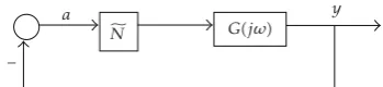
Figure 1: Feed back configuration for nonlinear systems.

techniques is the need to understand the behavior of nonlinear systems, which in turn is based on the simple fact that every system is nonlinear, except in very limited operating regimes. The basic philosophy of DF is to replace each nonlinear element with a quasi-linear descriptor or describing function. The functional form of such a descriptor is governed by several factors, the type of input signal, which is assumed in advance, and the approximation criterion, for example, minimization of mean squared error. This technique is dealt with very thoroughly in a number of texts for the case of nonlinear systems with a single nonlinearity 4. One category of DFs that has been particularly successful is the sinusoidal input describing functionSIDF.

The fundamental ideas and use of the SIDF approach can best be introduced by overviewing the most common application, limit cycle analysis for a system with a single nonlinearity. A limit cycleLCis a periodic signal,xLCtT xtfor alltand for some

T the period, such that perturbed solutions either approach xLC a stable limit cycle or diverge from itan unstable one. Recently several analytical techniques have been proposed in the framework of the Bifurcation theory for investigating different aspects of limit cycle operation5,6. Nonlinear techniques for modeling the periodic signal in general and limit cycles in particular have also been suggested7. However, an approach to LC analysis that has gained widespread acceptance is the graphical frequency-domain SIDF method8,9.

In this paper the describing function method is first extended to the case of single input single outputSISO systems, where the condition for elementary SIDF application is not strictly satisfied10. When the linear system element does not attenuate the super-harmonic components around the feedback loop, the input to the nonlinear element will not be a pure sinusoid and will be a distorted waveform containing higher harmonics. The first part of this paper uses theDFM, to account for higher harmonics and widen the scope of applications of the SIDF method11.

The second part of the paper further extends the SIDF techniques to a class of multiloop nonlinear systems in which the nonlinear elements are separable from the linear part. In both cases, emphasis is placed on the multiobjective formulation of predicting the limit cycle operation and the subsequent solution of the harmonically linearised system equations by the multiobjective genetic algorithmsMOGA.

2. Harmonic Analysis

The harmonic balance equation for the autonomous feedback configuration of Figure 1, in which the nonlinearity exists as a separable element in an otherwise linear system, is given as

1Na, ωGjω 0, 2.1

of2.1is sought. However, the valid application of the SIDF requires that the input signal to the nonlinear element be essentially sinusoidal in form. This is a condition which imposes an overall low-pass frequency characteristic on the linear system elements such that the super-harmonic signals are attenuated around the feedback loop. Based on the assumption that the input to the nonlinear element is a pure sinusoidal, the SIDF is derived as

Na, ω

b1jc1

ejωt

aejωt

1

a

b1jc1

, 2.2

whereb1 and c1 are the first harmonics in the Fourier series ofN, andais the amplitude of the input sinusoidal. In general the SIDF is a function of both input amplitude and input frequency, however, for single valued, sector bounded nonlinearities which are the subject of this work, the describing function is real and only a function of input amplitudea, therefore for brevityNais used to denote the SIDF.

3. Extension of Higher Harmonic Analysis to SISO Systems

In cases where the requirements of the overall low-pass characteristics of the linear system elements are met, the conventional graphical technique in the frequency domain has been shown to give acceptable results 9. This elementary SIDF analysis and the associate graphical solution are well documented4. However, in those cases where the amplitude of higher harmonics of the Fourier series at the output of the nonlinear element are significant and are not suppressed around the feedback loop, the key assumption in derivation of the SIDF is violated 10. The reason being that the input to the nonlinear element will be a distorted waveform containing the fundamental as well as other harmonics. One method to remedy this circumstance is to find error bounds for the elementary SIDF. Based on Tsypkin’s method, a strategy with which to find systems with a low-pass linear part for which the describing function technique erroneously predicts limit cycles is outlined in10. A more attractive method that widens the scope of the SIDF applications, as well as achieving a more accurate limit cycle prediction is to account for additional harmonics. An appropriate technique is the so called “describing function matrix” DFM, which is a mathematical formulation that allows an arbitrary number of harmonics to be taken into account in the SIDF analysis11,12.

Consider a nonlinear elementN which gives outputy Nxfor an inputx. It is required to examine the behavior ofNunder an input which is exactly periodic. Let this be

xRe

_∞

r0

arejrωt

, 3.1

where a a0, a1, a2. . .T is the vector of amplitudes of the harmonic components at the input to the nonlinear element and for a finite number of harmonics r m, am a0, a1, a2, . . . , amT,T denotes transposition ofa. LetCbe an analogous vector of complex

Fourier coefficients of the nonlinearity outputy, then an infinite matrixN the describing function matrixmay be defined as follows:

The 0th column is given byNk0Ca0/a0,

where, for example, the 3.1, 2.1 element represents the amplitude of the 3rd output harmonic divided by that of the 1st input harmonic. In general, thejth column is given by,

Nkj _C

k

aj

−Ck

aj−1

aj

, 3.2

whereksignifies the row number and is the index of harmonic components. If the nonlinear element is not frequency dependent and no bias level is present, then the 0th column can be ignored, and in this case the first element of the first column is the normal SIDF. Also note that if the nonlinear element is symmetrical and odd valued, then even rowsk2,4,6, . . .

can be ignored.

Now define the linear part Gm _{Diagg0jω, gjω, gj2ω, . . . , gjmω and}

representing the nonlinear element with DFM formharmonic components, the condition for existence of oscillation is that the following simultaneous harmonic balance equation3.3

INmGmam0 3.3

has a solutionψm _aωm. The reason forGbeing a diagonal matrix is that different harmonics

do not interact in passing through the linear element.

Consider the nonlinear SISO system shown in Figure 1 in which GjωandNa

are scalars. Assume a fundamental plus a third harmonic to be present at the input to the nonlinear element. Further, assume that the nonlinear element is not frequency dependent, but is symmetrical and odd valued function. The describing function matrix for an input of the following form

xt a1sinωta3sin3ωtφ 3.4

can be constructed as

N

⎡ ⎢ ⎢ ⎢ ⎣

c1

a1

a1

c1

a1, a3

−c1

a1

a3

c3

a1

a1

c3

a1, a3

−c3

a3

a3

⎤ ⎥ ⎥ ⎥

⎦, 3.5

where φ is the phase shift between the two harmonics andc1a1, c3a3are respectively, the first and the third coefficients of Fourier components at the nonlinear output, due to the componenta1sinωtonly, andc1a1, a3, c3a1, a3are the corresponding coefficients due to the sum of the two signals at the input to the nonlinear element.

In the case of only two harmonics such asxtgiven by3.4, the harmonic balance equation3.3is reduced to the following two simultaneous equations

whereN2_{is the second orderfirst and the third harmonicDFM andG}2_{is a 2×2 diagonal} matrix 1 0 0 1 n11 a1 n12

a1, a3

n21 a1 n22

a1, a3

gjω 0

0 gj3ω

a1

a3∠φ

0, 3.7

equation3.7may be written as

1n11

a1

gjωa1n12

a1, a3

gj3ωa3∠φ0,

n21

a1

gjωa1

1n22

a1, a3

gj3ωa3∠φ0,

3.8

wheren11, n12, n21, n22represent the elements of matrixNas defined by3.5. Rearranging the second equation in the equation set3.8

a3∠φ−

n21

a1

gjω

1n22

a1, a3

gj3ω

a1. 3.9

A search has to be carried out in the space ofa1, φ, ω, a3in that orderto find those values of

a3andφwhich will satisfy3.9. If such values are found, the result will be substituted into the first equation of equation set3.8, to test for this equation which governs the fundamental oscillation.

Substituting3.9into the first equation of equation set3.8and rearranging yields

n11

a1

gjωa1G1−1, 3.10

where G1 −n12a1, a3gj3ωn21a1gjω/1 n22a1, a3gj3ω,3.10 represents the overall harmonic balance equation for both the fundamental and the third harmonic components. Hence, a limit cycle with parametersa1, a3, ω, φ exists when the following two equations are simultaneously satisfied;

n11

a1

gjωa1G11,

∠n11

a1

gjωa1G1

180±2kπ, k0,1, . . . . 3.11

Alternatively,3.8may be rearranged as follows and be directly used as the objectivefitness functionin the subsequent MOGA search as the satisfaction of these objectives implies the solution of the two simultaneous harmonic balance equations3.8

Obj₁1n11

a1

gjωa1n12

a1, a3

gj3ωa3expjφ≤ε, Obj₂n21

a1

gjωa1

1n22

a1, a3

gj3ωa3expjφ≤ε.

3.12

space ofa1, a3, ω, φto facilitate an efficient and an accurate prediction of limit cycle in the presence of higher harmonics.

4. Extension of Harmonic Analysis to MIMO System

Extension of describing function techniques to multiloop nonlinear systems is not new and follows the development of the frequency domain multivariable linear theory13,14. A numerical technique with a graphical interpretation for quantifying the limit cycle parameters in multivariable systems in the frequency domain is reported in 15. The extension of the graphical techniques to multiloop systems with coupled multivalued nonlinear elements is reported in 16. Another graphical method based on the phasor diagram which particularly gives accurate limit cycle prediction for relay systems is developed in 8. A computer aided design CAD tool for limit cycle prediction aimed at educational purposes is reported in 9. Another novel numerical technique based on deriving the least damped eigenvalue to the imaginary axis for nonlinear systems with multiple nonlinearities is suggested in 17. Based on defining an appropriate error function, the authors use both eigenvalue and eigenvectors to formulate a generalized Newton-Raphson method to solve for the state variable amplitude in a minimum norm sense 17. Most of the above mentioned techniques are essentially dependent on the graphical displays in the frequency domain. While this is useful for getting insight into the subsequent compensator design, an efficient technique for accurately quantifying the limit cycle parameters is still highly desirable.

In this paper, a multiobjective formulation is presented to search numerically for limit cycles in a class of multiloop nonlinear systems. The approach is computationally efficient and is based on multiobjective genetic algorithmsMOGA.

5. Limit Cycle Prediction in Nonlinear Multivariable Systems

Provided that certain limitations are placed on the form of the linear system elements, the extension of the of harmonic linearization to multivariable systems is conceptually straight-forward. The equation governing limit cycle operation in the autonomous multivariable nonlinear feedback system ofFigure 1can be expressed as

Ta, jω Ia0, 5.1

whereTa, jω Na, jωGjω andNa, ωis the matrix of sinusoidal input describing function corresponding to the nonlinear elements ofN, and ais the column vector of the sinusoid at the inputs to these elements. The use of a single sinusoidal describing function analysis implies the following assumptions:

aEach element of Gjωacts as a low pass system so that higher harmonic signal components are effectively suppressed.

Equation5.1will have a nontrivial solution only if

detNa, ωGjω I 0. 5.2

Thus for no limit cycle to exist, no eigenvalue ofNa, ωGjωcan equal−1,j0.

The conventional graphical frequency domain method for the solution of 5.2 for single input single output systems with a single nonlinear element may be extended to MIMO systems employing Nyquist or the Inverse Nyquist Array. Invoking the Inverse Nyquist Array method13, the possibility of limit cycle existence may be examined by studying the following inequalities:

nkk

ak

gkkjω>

j /k

njk

ak

gjkjω,

5.3

_nkk

ak

gkkjω>

j /k

_njk

ak

j /k

gjkjω, _5.4

where njka and gjkjω are the jkth elements of the matrices, Na for single valued

nonlinear elements and G−1_{jω, respectively. Inequality 5.3 implies that no limit cycle} operation is theoretically possible if Gershgorin bands associated with each diagonal element ofNaG−1_{jωdo not encompass the origin in the complex frequency domain. Inequality}

5.4implies the same result, provided that the bands traced out by the Gershgorin discs on the loci of giijω and niia do not intercept for every i. The former representation

is computationally more demanding, but gives less conservative results because of the weakening step between inequalities5.3and5.4. The Gershgorin discs set bounds to the eigenvalue locations and any method of limit cycle prediction based on band intersection should have a tendency to be conservative.

An alternative approach lies in calculating eigenvalue of the harmonically linearised return ratio system equation. For a general system which contains both on and offdiagonal nonlinear elements, the computational effort involved in determining the eigenvalue becomes almost formidable as, at any frequency, the return ratio matrix is a function of the signal amplitude at the input to the nonlinear elements16.

A numerically based technique called the sequential loop balance method has also been devised15. This method is based on5.1for whichTa, jωhas elements of the form

tijaj, jω, andais a column vector at the input to the nonlinear elements such that aj Ajexpjφi, j1,2, . . . , n, for allj, i1,2, . . . mover arbitrary rangesA, ω, andφ, a possible

infinite number of solutions may exist for 5.1. For a specified value of frequency and a specified range of discrete values of the reference signala1 A1ej0, A1 > A2, A3, . . . , An a

finite number ofpsets of sinusoidsa1k, a2k, . . . , ank, k 1,2, . . . , p which will satisfy the

condition for harmonic signal balance in thenth system loop as given by5.5are found;

tnn1

an n−1

j1

tnjaj0. 5.5

−

−

n11

n21

n12

n22

g11

g21

g12

g22

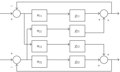
Figure 2: A two-input two-output nonlinear system.

sinusoids and the process is repeated in a sequential manner until loop 1 is reached. Clearly this method is also computationally demanding due to an indirected search over the specified ranges of parameters. Further, it does not search for the phase difference between the oscillating loops, and as discrete data are used in the computation, there is the possibility of solution sets which exist over the data intervals.

Considering the 2×2 autonomous system shown in Figure 2, the set of equations governing this model is given by5.6

1n11

a1

g11jω

a1n21

a2

g21jωa2ejφ0,

n12

a1

g12jωa11n22

a2

g22jω

a2ejφ0.

5.6

In this case there are two equations and four variablesunknown. The solution of these equations is sought over a range of specific values ofa1, a2, ωand ϕ, wherea1 and a2 are amplitudes of limit cycles in loop 1 and 2, respectively,ωis frequency of oscillation for both loops andφis the phase-shift between the loops.

6. Multiobjective Genetic Algorithms

18, although several multiobjective schemes have been proposed 19, 20. Applications of multiobjective evolutionary schemes to control systems analysis and design have been widespread 21, 22. A formulation called the multiobjective genetic algorithm MOGA maintains the genuine multiobjective nature of the problem, and is essentially the scheme adapted here23. Further details for the MOGA can be found in20. The design philosophy of the MOGA differs from other methods in that a set of simultaneous solutions are sought and the designer then selects the best solution from the set. The idea behind the MOGA is to develop a population of Pareto-optimal or near Pareto-optimal solutions. The aim is to find a set of solutions which are nondominated and satisfy a set of inequalities. An individual j with a set of objective functionsϕj _ϕj

1, . . . , ϕ

j

nis said to be nondominated if for a population

of N individuals there are no other individualsk1, N;k /jsuch that

a ϕk

i ≤ϕ j

i ∀i1,2, . . . , n,

b ϕk_i < ϕj_i for at least onei. 6.1

The MOGA is set into a multiobjective context by means of the fitness function. Individuals are ranked on the basis of the number of other individuals they are dominated by for the unsatisfied inequalities. Each individual is then assigned fitness according to their rank. The mechanism is described in detail in20. To summarize, the MOGA problem could be stated as:

Find a set of Madmissible pointsPj, j 1, . . . , Msuch that

ϕj_i ≤εi j 1,2, . . . , m, i1,2, . . . , n. 6.2

And such thatϕj_{j1, . . . , Mare nondominated.}

Genetic algorithms are naturally parallel and hence lend themselves well to multiobjective settings. They also work well on nonsmooth objective functions. Thus MOGA can be used to search the existence of any possible limit cycle operation in nonlinear MIMO systems.

7. Applications

7.1. SISO System

The feedback configuration of the single input single output system considered in this example is shown inFigure 3.

A Fourier analysis of the nonlinearity output shows that the amplitude of the third harmonic component is significant. Therefore, the elementary describing function analysis does not give accurate limit cycle prediction. Based on the calculation of the required Fourier coefficients at the output of the nonlinear element for the input of the form given by3.4, the describing function matrix as defined by3.5is derived as,

DFM

⎡ ⎢ ⎢ ⎢ ⎣

1.91

a1

−1.12

a3 0.64

a1 0.89

a3

⎤ ⎥ ⎥ ⎥

−

0.5 1.5

0.5 0.75

2 ss0.4s1.0

Figure 3: SISO nonlinear feedback system.

Table 1: MOGA parameters for the SISO system.

Number of generation

Population size

Selection method

Representation method

Multiobjective method

Mutation probability

Cross over probability

50 100 Tournament Binary 8 bit for

each parameter Pareto 0.02 0.7

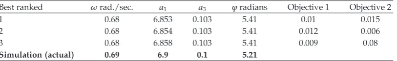
Table 2: Results of limit cycle prediction with MOGA for SISO system.

Best ranked ωrad./sec. a1 a3 ϕradians Objective 1 Objective 2

1 0.68 6.853 0.103 5.41 0.01 0.015

2 0.68 6.854 0.103 5.41 0.012 0.006

3 0.68 6.858 0.103 5.41 0.009 0.08

Simulationactual 0.69 6.9 0.1 5.21

a1anda3denote the amplitude of the first and third harmonics at the input to the nonlinear element. The harmonic balance equation is formulated in the presence of the third harmonic using3.12withε0.01. The range of limit cycle parameters are specified as

0.1≤ω≤1.5, 3≤a1≤8.0, 0.05≤a3≤0.5, 0.1≤φ≤2π. 7.2

The population is initialized randomly and the MOGA program is run to search the space of these parameters for the simultaneous satisfaction of objectives3.12. The parameters of MOGA are shown inTable 1and after 18 generations the algorithm converged with the value ofε0.012. The first three solutions are ranked based on the concept of non dominance and are listed inTable 2. The results obtained from simulation are also shown in bold inTable 2

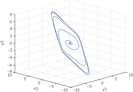
and are comparable with those predicted by MOGA. The phase space of the predicted limit cycle is shown inFigure 4.

−10 −5

0 5

10

x1

−10 −5 0 5 10

x2

−8 −6 −4 −2 0 2 4 6 8

x

3

Figure 4: Phase space of limit cycle for SISO example.

7.2. MIMO Systems

In this section, two 2×2 nonlinear systems are presented. In the first example the elements of the nonlinear matrix are similar and consist of four ideal relays.

In both examples the numerical solution of 5.6 is formulated as a 2-objective problem, and the satisfaction of these objectives implies the solution of the simultaneous harmonic balance5.6

Obj₁ 1n11

a1

g11jω

a1n21

a2

g21jωa2eφ≤ε,

Obj₂n12

a1

g12jωa1

1n22

a2

g22jω

a2ejφ≤ε,

7.3

where Obj₁and Obj₂are the values of the right-hand side of5.6which ideally should tend towards zero for specific values ofa1, a2, ω, andφ. Upper and lower bounds are specified for ω, a1, a2, and φ, then the real generational MOGA with specified selection method, cross over, mutation rate and population size is called to search over the parameter space of

ω, a1, a2, andφ. The required numerical accuracy may be achieved by specifying the number of genesbinary bitsfor each individual in accordance with the value ofε. If conditions for inequalities7.3exist, then MOGA converges to the correct values of limit cycle parameters after a number of generations. If finer and more accurate parameter values are required, the bounds on the parameters ω, a1, a2, and φ may be tightened and the number of genes increased on the subsequent run of the MOGA program. In order to avoid the local minima and premature convergence the mutation probability rate may be taken higher at the beginning and decreased exponentially toward the end of the run. One advantage of limit cycle prediction based on MOGA is that multiple solutions may be distinguished by using the Niching mechanism19.

−1 1

Input Output

Figure 5: Ideal relay-nonlinear elements for MIMOExample 7.1.

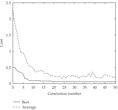
0 5 10 15 20 25 30 35 40 45 50 Generation number

0 0.5 1 1.5 2 2.5

Cost

Best Average

Figure 6: Convergence curve for MIMOExample 7.1.

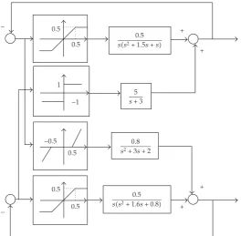
Example 7.1. The nonlinear control system with two inputs and two outputs has the

configuration ofFigure 2 with four similar nonlinear elementsn11 n12 n21 n22 of the form shown inFigure 5.

The linear system matrix is

G

⎡ ⎢ ⎢ ⎢ ⎣

0.5

ss2_1.5s0.5

−0.15

s2_s1

0.8

s2_3s2

1

ss2_1.6s0.8

⎤ ⎥ ⎥ ⎥

⎦. 7.4

0 10 20 30 40 50 60 70 80 90 100 Timeseconds

−2 −1.5 −1 −0.5 0 0.5 1 1.5 2

Amplitude

y1 y2

Figure 7: Simulation results for MIMOExample 7.1.

Table 3: MOGA parameters for MIMOExample 7.1.

Number of generation

Population size

Selection method

Representation method

Multiobjective method

Mutation probability

Cross over probability

50 50 Tournament

Binary 8 bit for each

parameter

Pareto 0.02 0.7

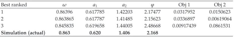
Table 4: Results of limit cycle prediction with MOGA forExample 7.1.

Best ranked ω a1 a2 ϕ Obj 1 Obj 2

1 0.86396 0.617785 1.42203 2.17477 0.0317952 0.0150623

2 0.863865 0.617787 1.41485 2.15623 0.0336897 0.00619064

3 0.845835 0.619658 1.44005 2.48668 0.00917439 0.0861531

Simulationactual 0.863 0.620 1.406 2.168

range of the parameters feasible solutions exist, MOGA converges to solutions which are ranked according to their fitness values measured by the concept of non dominance, that is, Pareto optimal. For a population size of 50, it was observed that initially a large number of solutions exist. However, as the search progressed most members of the population tend to be concentrated around a narrow range of parameters. After 25 generations the algorithm converged and the results for the first three solutions are given inTable 4and the convergence curve is shown inFigure 6. InFigure 6 the cost axis is a measure of fitness and the doted curve represent the sum of the average of the two objectives average Obj₁ Average

Obj₂and the solid curve represent the sum of the best values of the two objectivesbest

− _0.5 0.5

0.5 ss2_1.5ss

1 −1

5 s3

−0.5 0.5

0.8 s2_3s2

−

0.5 0.5

0.5 ss2_1.6s0.8

Figure 8: Two dimensional nonlinear systems forExample 7.2.

Table 5: Results of limit-cycle prediction with MOGA for MIMOExample 7.2.

ω a1 a2 ϕ Obj 1 Obj 2

1 0.517728 1.18528 1.73296 3.6772 0.0229142 0.0611446

2 0.517638 1.18025 1.73396 3.67718 0.0181093 0.0655828

3 0.530139 1.16228 1.68292 3.67689 0.0410611 0.0383831

Simulationactual 0.5400 1.073 1.543 3.500

In order to validate the results given byTable 4, the nonlinear system was simulated. The results of simulationactual LCcompare well with the results obtained by MOGA. This is also shown in bold inTable 4and inFigure 7. The reason for the very accurate limit cycle prediction in this example is two folds, one is that all nonlinear elements have the same characteristics and the other is that the linear system elements have a low pass frequency characteristics.

Example 7.2. The nonlinear system for this example is of the same configuration as inFigure 2, and is shown inFigure 8. In this case the nonlinear matrix consists of different nonlinear behavior such as saturation, ideal relay, and dead zone.

The same MOGA parameters were chosen as inTable 3and the following ranges were specified for the parameters

0 10 20 30 40 50 Generation number

0 0.5 1 1.5 2 2.5 3

Cost

Best Average

Figure 9: Convergence curve for MIMOExample 7.2.

0 20 40 60 80 100

Timeseconds −2

−1.5 −1 −0.5 0 0.5 1 1.5 2

Amplitude

y1 y2

Figure 10: Simulation results for MIMOExample 7.2.

For this example, the algorithm converged within 30 generations, consuming 31.2 seconds of CUP time on the same machine. For all 50 generations 52 seconds of the CPU time is consumed on the same machine. The convergence curve is shown inFigure 9.

not strictly conform to the filter hypothesis, thus reducing the describing function accuracy and hence the reason for the small discrepancy between simulation and MOGA results. The development of similar analysis as for SISO systems will improve the SIDF accuracy significantly.

8. Conclusion

The single sinusoidal input describing function is extended by means of describing function matrix to account for higher harmonic signal components. In the analysis of single loop nonlinear systems, the describing function matrix provides a rigorous method, enhances limit cycle prediction and widens the scope of the valid application of the SIDF to those cases for which the assumption of the filter hypothesis is not strictly met. It is shown how, by formulating limit cycle prediction in the presence of higher harmonics as a multiobjective problem and using the MOGA procedure, a solution to the DF matrix equation can be obtained efficiently in numerical form. This is useful in illustrating both how a multiplicity of possible solutions may arise, and for emphasizing the effects of higher harmonic signal content.

Next, the single sinusoidal input describing function technique is extended to multiloop nonlinear systems. For the class of separable nonlinear elements of any general form, the linearized harmonic balance equations are derived. The search for limit cycle is formulated as a multiobjective problem. The multiobjective genetic algorithm is employed to obtain quantitative values for parameters of possible limit cycle operation. The MOGA search space is the space of the limit cycle parameters such as amplitudes, frequency and phase difference between the interacting loops. The algorithm is computationally efficient and provides very accurate results when the conditions for the SIDF application are satisfied. In both cases of SISO and MIMO systems, emphasis is placed on the formulation of limit cycle parameters as a multiobjective problem and subsequent solution by the evolutionary MOGA method. Finally, examples of use are given to demonstrate the effectiveness of the proposed approach.

References

1 R. Hilborn, Chaos and Nonlinear Dynamics, Oxford University Press, Oxford, UK, 2001.

2 M. Vidyasagar, Nonlinear Systems Analysis, vol. 42 of Classics in Applied Mathematics, SIAM, Phi-ladelphia, Pa, USA, 2nd edition, 2002.

3 H. Khalil, Nonlinear Systems, Prentice-Hall, Upper Saddle River, NJ, USA, 3rd edition, 2002.

4 J. H. Taylor, “Describing functions,” in Electrical Engineering Encyclopedia, John Wiley & Sons, New York, NY, USA, 1999.

5 M. Basso, R. Genesio, and A. Tesi, “A frequency method for predicting limit cycle bifurcations,”

Nonlinear Dynamics, vol. 13, no. 4, pp. 339–360, 1997.

6 F. Angulo, M. di Bernardo, E. Fossas, and G. Olivar, “Feedback control of limit cycles: a switching control strategy based on nonsmooth bifurcation theory,” IEEE Transactions on Circuits and Systems I, vol. 52, no. 2, pp. 366–378, 2005.

7 E. Abd-Elrady, Nonlinear approaches to periodic signal modeling, Ph.D. thesis, Division of Systems and Control, Department of Information Technology, Uppsala University, Uppsala, Sweden, January 2005.

8 K. C. Patra and Y. P. Singh, “Graphical method of prediction of limit cycle for multivariable nonlinear systems,” IEE Proceedings: Control Theory and Applications, vol. 143, no. 5, pp. 423–428, 1996.

10 S. Engelberg, “Limitations of the describing function for limit cycle prediction,” IEEE Transactions on

Automatic Control, vol. 47, no. 11, pp. 1887–1890, 2002.

11 A. I. Mees, “The describing function matrix,” IMA Journal of Applied Mathematics, vol. 10, no. 1, pp. 46–67, 1972.

12 S. D. Katebi and M. R. Katebi, “Combined frequency and time domain technique for the design of compensators for non-linear feedback control systems,” International Journal of Systems Science, vol. 18, no. 11, pp. 2001–2017, 1987.

13 H. H. Rosenbrock, Computer-Aided Control System Design, Academic Press, New York, NY, USA, 1974.

14 A. G. J. MacFarlane and J. J. Belletrutti, “The characteristic locus design method,” Automatica, vol. 9, pp. 575–588, 1973.

15 J. O. Gray and P. M. Taylor, “Computer aided design of multivariable nonlinear control systems using frequency domain techniques,” Automatica, vol. 15, no. 3, pp. 281–297, 1979.

16 S. D. Katebi and M. R. Katebi, “Control design for multivariable multivalued nonlinear systems,”

Systems Analysis Modelling Simulation, vol. 15, no. 1, pp. 13–37, 1994.

17 V. K. Pillai and H. D. Nelson, “A new algorithm for limit cycle analysis of nonlinear control systems,”

Journal of Dynamic Systems, Measurement, and Control, vol. 110, no. 3, pp. 272–277, 1988.

18 D. E. Goldberg, Genetic Algorithms in Search, Optimization and Machine Learning, Addison-Wesley, Reading, Mass, USA, 1989.

19 K. Deb, Multi-Objective Optimization Using Evolutionary Algorithms, Wiley-Interscience Series in Systems and Optimization, John Wiley & Sons, Chichester, UK, 2001.

20 C. A. Coello Coello, D. A. Van Veldhuizen, and G. B. Lamont, Evolutionary Algorithms for Solving

Multi-Objective Problems, vol. 5 of Genetic Algorithms and Evolutionary Computation, Kluwer Academic

Publishers, New York, NY, USA, 2002.

21 G. P. Liu, J. B. Yang, and J. F. Whidborne, Multi-Objective Optimisation and Control, Research Studies Press, Baldock, UK, 2003.

22 Mo. Jamshidi, L. D. Santos Coelho, R. A. Krohling, and P. J. Fleming, Robust Control Design Using

Genetic Algorithms, CRC Press, Boca Raton, Fla, USA, 2002.

23 C. M. Fonseca and P. J. Fleming, “Multi-objective genetic algorithms,” in Proceedings of the IEE