On the Convex Feasibility Problem

(1)

Anale. Seria Informatică. Vol. VII fasc. 1 – 2009

Annals. Computer Science Series. 7th_{Tome 1}st_{Fasc. – 2009}

O

n

t

h

e

C

o

n

v

e

x

F

e

a

s

i

b

i

l

i

t

y

P

r

o

b

l

e

m

Laura Măruşter1 and Ştefan Măruşter2 1

University of Gröningen, Gröningen, Nederland

[email protected]

2

West University of Timişoara, Romania

[email protected]

ABSTRACT. The convergence of the projection algorithm for solving the convex feasibility problem for a family of closed convex sets, is in connection with the regularity properties of the family. In the paper [18] are pointed out four cases of such a family depending of the two characteristics: the emptiness and boudedness of the intersection of the family. The case four (the interior of the intersection is empty and the intersection itself is bounded) is unsolved. In this paper we give a (partial) answer for the case four: in the case of two closed convex sets in 3 the regularity property holds.

KEYWORDS: Convex feasibility problem, Strong convergence, Regularity properties.

Introduction

The convex feasibility problem can be formulated in a very simple way: Let

Ai, i=1,...,m, be a family of closed convex sets with nonempty intersection,

≠ ∩

i

A Ø, in a real Hilbert space; the convex feasibility problem is:

Find a point in∩A_i_.

(2)

process. A first result for solving the convex feasibility problem in this case was given by Agmon, Motzkin and Schoenberg in 1954, [1, 20].

In the last decades a number of papers were written on the subject and results concerning some theoretical aspects and particularly algorithms for solving this problem were obtained. The interest for the convex feasibility problem is motivated by some important applications in specific areas. In the paper [2] are pointed out the main applications both in other mathematical algorithms and directly in some practical problems; we list here a part of them.

Best approximation with applications in linear prediction theory, partial differential equations (Dirichlet problem), complex analysis (Bergman kernels, conformal mappings);

Subgradient algorithms with application in solution of convex inequalities, minimization of convex nonsmooth functions;

Image reconstruction, discrete and continuous models with applications in radiation therapy treatment planing, electron microscopy, computerized tomography, signal processing.

Usually, the convex feasibility problems are solved by projection algorithms. The geometric idea of the projection method is to project the current iteration onto certain set form the intersecting family and to take the next iteration on the straight line connecting the current iteration and this projection. A weight factor gives the exact position of the next iteration. Different strategies concerning the selection of the set onto which the current iteration will be projected, will give particular projection-type algorithms.

If P (x)

i

M denote the projection of x onto Mi, then the classical

projection method is

) ( )

1 (

) (

1 k k k M k

k t x t P x

x

k

α + −

=

+ (1)

where tk is the weight factor, 0 < tk < 2, and the function α_: _→_{1,…,_N_} defines the strategy. The usual strategy is the cyclic covering of the sets of the family, that is α(_k)=_mod_N(_k)+1

(3)

I

m_i Mi

M

1

=

= _{. A complete and exhaustive study on algorithms for solving}

convex feasibility problem, including comments about their applications and an excellent bibliography, was given by Bauschke and Borwein [2].

The paper is organized as follows. In section 2 we briefly state the convergence properties of the Mann iteration process. The projection algorithm is a particular case of this iteration, so that its convergence results from general theorems of the Mann iteration. Section 3 is devoted to regularity properties of a family of closed convex sets, properties which play a significant roll of the behavior of the sequence generated by this algorithm.

1 The projection algorithms and normal Mann iteration

The projection method is a particular case of the Mann iteration process:

) ( )

1 (

1 k k k k

k t x tT x

x ₊ = − + ₍₂₎

where tk is a sequence of real numbers satisfying some properties, usually called the control sequence. The convergence properties of the projection algorithm for convex feasibility problem are obtained from the general convergence properties of the Mann iteration.

Remark 1. Note that (2) is a particular case of the general Mann iteration )

(

1 k

k T x

x ₊ = _{, where} k _j

j kj

k x

x =

∑

₌

0α and A={αkj} is a triangular averaging

matrix. If this matrix satisfies the segmenting condition, that is,

nj n n j

n α α

α ₍₁ ₎

1 , 1 ,

1 + +

+ = − , then the general Mann iteration becomes just (2)

with a specific relaxation strategy, t_k = _k₊ _k₊ _,∀k∈N

1 , 1

α _{. If 0 <}_t_k_{< 1, then}

xk+1 is a convex combination of xk and T(xk). This restriction concerning {tk} is not always satisfied; the typical case is, for example, the projection algorithm for convex feasibility problem, algorithm which has the form (2) with 0< tk < 2. In particular, if ₌ ₂1

k

t , (2) becomes xk+1=(xk+T(xk))/2, which is the well known Krasnoselski method. The term Krasnoselski/Mann or the relaxed iteration is sometimes used for (1.2) as well.

(4)

will denote the set of fixed point of T in C, set which we will suppose throughout this paper to be nonempty.

Definition 1. The mapping T is said to be qusi-nonexpansive if ) ( * , ,

* *

)

(x x x x x C x FixT

T − ≤ − ∀ ∈ ∈

Definition 2. The mapping T is said to be demicontractive (or k -demi-contractive) if there exists k < 1 such that

) ( * , ,

* *

)

(x x 2 x x 2 T(x)-x 2 x C x Fix t

T − ≤ − +_k ∀ ∈ ∈ ₍₃₎

Obviously, the class of demicontractive mappings properly includes the class of quasi-nonexpansive mappings for 0≤_k≤1

Remark 2. For negative values of k the class of demicontractive mappings is diminished in a great extent; in [2] such a class (with negative value of k) was considered under the name of strongly attracting map. In particular, the mapping T which satisfied (3) with k = -1 is called pseudo-contractive in [26]. Note also that a mapping T satisfying (3) with k = 1 is usually called hemicontractive and it was considered by some authors in connection with strong convergence of the implicit Mann-type iteration (see, for example, [23]).

The notion of quasi-nonexpansivity was introduced by Tricomi in 1916 [25] for a real function f defined on a finite or infinite interval (a,b) with the values in the same interval. He proved that the sequence {xk} generated by the simple iteration xk+1=f(xk), x0-given in (a,b), converges to a fixed point of f provided that f is continuous and strictly quasi-nonexpansive on (a,b). Stepleman in a paper published in 1975 [24] studied necessary and sufficient conditions for the convergence of this sequence in real case. His main result states that convergence is assured if and only if the second iterate of f is strictly quasi-nonexpansive. The importance of the concept of quasi-nonexpansivity for the computation of fixed points in more general cases had been emphasized by many authors (see, for example, the survey papers of Petryshyn and Williamson [22] and of Diaz and Metcalf [7]) and this class of mappings is still being studied extensively (see, for instance, the recent monographs of Chidume [5] and Berinde [3] and the references therein).

(5)

Definition 3. A mapping T is said to be demiclosed at y, if for any sequence {xk} which converges weakly to x, and if the sequence {T(xk)} converges strongly to y, then T(x)=y.

In the sequel, as often as not, only the demiclosednes at 0 is used, which is a particular case when y=0.

The class of mappings satisfying the condition (3) and the name of demicontractive were introduced by Hicks and Kubicek in 1977 [10]. They studied the convergence properties of a sequence {xk} generated by the Mann-type iteration to a fixed point of T in real Hilbert spaces. They proved that if T is demicontractive and if I-T is demiclosed at zero, then the sequence {xk} generated by the Mann iteration (2) converges weakly to a fixed point of T. The control sequence is assumed to satisfy the condition

k

− < < →_t_, ₀ _t ₁

t_k .

In [15] a class of mappings which satisfies so called condition (A):

) ( * , ,

) ( *

),

(x x x x T x 2 x C x FixT

T

x− − ≥λ − ∀ ∈ ∈ (4)

where λ_{is a positive number was considered. It is routine to see that the} conditions (3) and (4) are equivalent λ=(1−k)/2 (indeed, it can be simply checked that x−x*2+_k x−T(x)2− T(x)−x*2 =2 x−x*,x−T(x)

2

) ( ) 1

( − x−T x

− _k _{). Thus the class of demicontractive mappings coincides}

with the class of mappings satisfying the condition (A). In [15], the same result concerning the weak convergence of the normal Mann iteration was obtained, more exactly, if T satisfies the condition (A) and I-T is demiclosed at zero, then the sequence {xk} converges weakly to a fixed point. The control sequence satisfies a similar condition (to a certain extent, weaker)

λ

2 0<_a≤_t ≤_b<

k (or 0<a≤tk ≤b<1−k). Note that the equiva-lence

between the conditions (3) and (4) was observed by some authors [12-14, 6, 21, 19]. Earlier, in 1973, in the paper [16], a similar result in a finite dimensional spaces was presented.

(6)

Definition 4. Let {xk} be a sequence in and let M ⊂ be a closed subset. We say that {xk} is regular with respect to M if _d(_x ,_M)→0

k

∞ →

k as

Theorem 1.(Petryshyn and Williamson) Suppose that _T_:_D⊂ → is

a quasi-nonexpansive mapping and that Fix(T) is nonempty and closed. Let D

x ∈

0 such that x =T(x0) ∈D,k =1,2,K

k

k Then the sequence {xk}

converges (strongly) to a fixed point of T if and only if {xk} is regular with respect to Fix(T).

Here, as usual, Tk denotes the kth iterate of T.

Remark 3. Theorem (1) is a slight generalization of the first result of [22] and its proof is, practically, identical. Essentially, Theorem (1) replaced the condition of continuity of T, from the original result, with the condition of closedness of Fix(T). It is easy to see that the latter condition is weaker, and, as will be seen, is essential for our development.

Consider now the following strategy in the projection algorithm. Let ix be the least index such that

) , ( max )

,

(x i x P x i P

x

i

x = −

−

This means that the current iteration is projected on one of the remotest sets of the family. Define the mapping T:→_by_T₍_x₎₌_P₍_x_,_i_{x). It is clear that}

i

M

x∈∩ _{if and only if}_T₍_x₎₌_x_{, hence if and only if}_x_{is a fixed point of}_T_, that is ∩M_i =Fix(T)_{. For any} _x∈ and x*∈Fix(T)_{, the following} Kolmogorov condition _x−_P(_x,_i ),_P(_x,_i )−_x* ≥0

x

x is satisfied and it is

routine to see that T is demicontractive and we get

2 2

2

) ( ) 2 ( * *

)

(x x x x t t x T x

T_t − < − − − − ₍₅₎

Therefore, Tt is quasi-nonexpansive. According to Theorem (1), the sequence {xk} given by the generation function Tt converges strongly to an element of Fix(T) if and only if _d _x _Fix _T → _as _k→∞

k, ( )) 0

(

On the other hand, it is easy to see that ( , )→0

i k M

x

d for each i. Indeed, from quasi-nonexpansivity of Tt it follows that the sequence

}

{x_k−y _is _monotone _decreasing _and _bounded, _therefore

∞ → →

−_y _as _k

x_k δ_y _{, for each}

i

M

(7)

) (

) 2 (

1 )

( 2 x y 2 x ₁ y 2 t

t x T

x_k _k _k− − _k −

− ≤

− ₊

and hence _x −_T _x → _as_k →∞

k

k ( ) 0 . But x−P(x,i) ≤ x−T(x) for each

i. Therefore _d₍_x_k_,_M_i₎= _x_k−_P₍_x_k_,_i₎ →₀ _as _k→∞_{and the essential} point in the convergence of the projection method is the following property of the family Mi: For any sequence {xk} such that d(xk,Mi)→ 0 for each i, one has d(xk,∩Mi)→0. Note that this property does not holds for any family (see the example below).

The above question was formulate by Gurin, Poliac and Raic [9] in 1967 in connection with strong convergence of the projection method. They proved that if ∩

_∩

≠

∈ )

( α α

α Int M

M _A Ø, where Mα is a certain set of the

family, then the family has the above property for any bounded sequence. In the sequel, we say that such a family has the GPR (Gurin, Poiac and Raic) property.

Bauschke and Borwein [2] introduced the notion of regularity for a finite family (N-tuple) of closed convex sets M1,...,MN with nonempty intersection M, by the condition

∈ ∀ > ∃ >

∀ε ₀_, δ ₀_, _x

δ

≤ =₁_, _, _} ),

, (

{d x M i N

max _i K

ε

≤ ⇒d(x,M)

If this holds only on bounded sets, then they speak of a boundedly regular family.

2 The regularity properties

In the paper [18] is pointed out that the GPR property of a family is in connection with the following two characteristics: the emptiness and the boundedness of the intersection of family. Therefore, the following four cases were

(1) Int∩ Mi ≠Ø and ∩Mi is bounded; (2) Int∩ Mi = Øand ∩Mi is unbounded, (3) Int∩ Mi ≠Ø and ∩Mi is unbounded; (4) Int ∩ Mi = Ø and ∩Mi is bounded.

(8)

holds (specific examples are given). The case 4 was left unsolved, the only remark that in this case the authors are looking for a suitable example is made. In the sequel we will prove that the GPR property holds for a particular family of sets with empty and bounded intersection (i.e. the case 4); so we give a partial answer for this case.

First of all we reproduce here the proof for the case 1 and the examples for the cases 2 and 3 from [17, 18].

Case (1). For the case of a bounded sequence, a similar result was given in [9].

Lemma 1. Let Mi ⊂ (i=1,…,m) be a family of convex sets such that Int ∩ Mi is nonempty and bounded and let {xk} be a sequence of such that _d _x _M → _as_k→∞

i

k, ) 0

( for each i. Then _d _x ∩_M → _as_k→∞

i

k, ) 0

( .

Proof. We assume that o∈Int∩Mi. Then there exists a closed ball D(o,r)= {x∈_:

i

M r

x ≤ _}⊂∩ _{. Let}_ε_{be a given real number, 0 <}_ε_{< 1, and}

let C be a constant such that _x ≤_C−1_{for all}_x∈ ∩Mi which is possible,

because ∩Mi is bounded.

Since, _d _x _M → _as_k →∞

i

k, ) 0

( for each index i, there exists a

sequence i _k _N _i

k M

y _}_∈ ⊂

{ () _{such that} ₋ _→ _→_∞

k as x

y_k(i) _k 0 _{. Let}

K , 1 , 0 ), )( 1 ( − ()− =

= _y _x _k

z k

i k C

k ε (6)

There exists a number ki(ε_{) such that if} _k≥_k_i₍ε₎_then

ε C r k i k x

y − ≤ ₋ 1 )

(

and so zk <r, that is zk ∈∩Mi.

On the other hand, from (6) we obtain

) ( ) 1 ( ) 1 ( i k k k y C z C x C ε ε ε − + = −

and for _k≥_k_i(ε)_{we have} _k _i

C x ∈M

− ₎ 1 ( ε

, because k i i

k z M

y()_, ∈ _and_M_i_are

convex.

Now, let k0(ε)=maxiki(ε). Then, for k≥k0(ε) it follows that

i k

C x ∈∩M

− ₎ 1 ( ε and ε ε ε ε

ε ₌ ₋ _<

− − ≤ ∩

− C k

C k C k

i

k M x x x

x

d( , ) (1 ) (1 )

(9)

Case (2). Example. Suppose that _{is the real three-dimensional}

space, that the set A1 is a cone and the set A2 is a tangent plane (ABCD) . The situation is depicted in Figure 1

Fig. 1.

The plane (ABCD) is tangent to the cone along the generatrix (AB) and hence A1∩A2=(AB). Now, let us consider a sequence {xk} in the plane (ABCD) such that d(xk,(AB)) = δ = const. and _x →∞_as_k→∞

k . It is

clear that _d _x _A → _as_k →∞

k, ) 0

( ₂ and _d(_x ,_A₁)=0

k for all k; but

0 )

,

(x A₁∩A₂ =δ >

d _k . Therefore, the conclusion of Lemma 1 is not true.

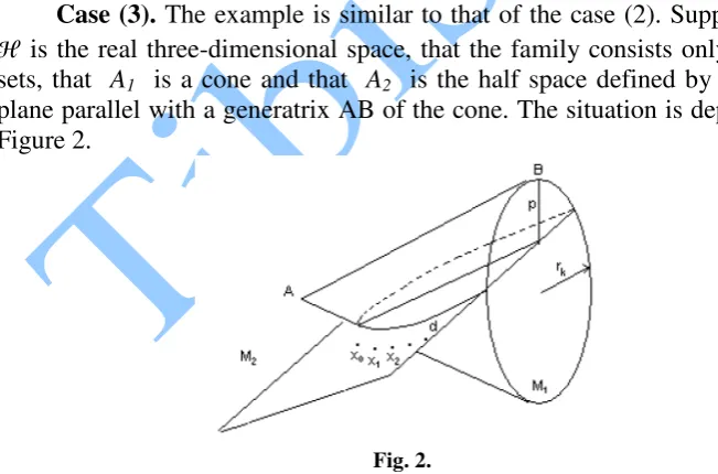
Case (3). The example is similar to that of the case (2). Suppose that

is the real three-dimensional space, that the family consists only of two sets, that A1 is a cone and that A2 is the half space defined by a secant plane parallel with a generatrix AB of the cone. The situation is depicted in Figure 2.

Fig. 2.

(10)

cone and plane. We have d(xk,A2)=0. By an elementary computation, the distance between the terms of the sequence and M1, is given by the formula

, 2

2 )

,

( 2 2 2

1 k k k

k M r d d pr p r

x

d = + + − −

where p, d, rk have the meaning from Fig. 1.

Therefore, d(xk, A1) → 0, whereas d(xk, A1∩A2) = d > 0.

Case (4). We will prove that for a particular case the GPR property holds. This particular case is: The Hilbert space is the Euclidean 3 dimensional space, the family consists in two closed convex sets, A and B, and the intersection A∩B is bounded and belongs to a plan _{(thus the}

interior of the intersection is empty).

Some preliminaries. Let A be a closed convex set in 3 and let (A,x)

be the convex cone hull of A with vertex x. Let d∈A and let r =x+t(d-x) be the ray with origin x passing though d. Let also td be a positive number defined by

) ( min )

(d x x t d x t

x

t

d − = + −

+

Definition 5. The superior side of (A,x) is

Sup (A,x)={x+t(d-x): 0≤t≤td, d∈ A}

Lemma 2. Let A be a closed convex set in 3, let x be a point such that

x∉A and let y be a point on the border of Sup (A,x). If Pxand Py denote the projection of x and y onto A respectively, then

x

y x P

P

y− ≤ −

Proof. Let z be a point in Ray(x,y)∩A. Because y belongs to the segment

[x,z], it follows that y = tx+(1–t) z, 0 ≤ t ≤ 1. Let u on be [x,z] given by y=tPx+(1–t)z; as x and Px are in A, it follows that u∈A. From Kolmogorow characterization of the projection it obtain _x−_P,_P −_z ≥0

x

x . On the other

hand, by a direct computation, it results

2 2

2

,

2 y P P u P u P

y u

y− − − _y ≤ − _y _y− + _y− _.

and y−P_y ≤ y−u _{. Therefore,}

x

x x P

P x t u y y P

(11)

Consider now the following enlargement of both sets A and B: Let x be a point does not belonging to A, and let Px be the projection of x onto A∩ B∈ . Suppose that Px∈ Int(A∩B). The symmetric point xs of x with respect to Px lay in the opposite side of , therefore xs ∉ B.

Let (A,x) and (B,xs) be the convex cone hulls of A and B with the vertex x and xs respectively; these cone hulls are our enlargements.

Lemma 3. The intersection (A,x) ∩ (B,xs) is bounded and has its interior nonempty.

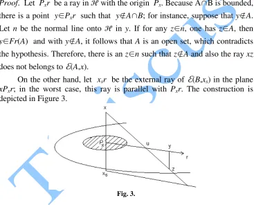
Proof. Let Pxr be a ray in with the origin Px. Because A∩B is bounded, there is a point y∈Pxr such that y∉A∩B; for instance, suppose that y∉A. Let n be the normal line onto _in_y_{. If for any}_z∈n, one has z∈A, then y∈Fr(A) and with y∉A, it follows that A is an open set, which contradicts

the hypothesis. Therefore, there is an z∈n such that z∉A and also the ray xz does not belongs to (A,x).

On the other hand, let xsr be the external ray of (B,xs) in the plane xPxr; in the worst case, this ray is parallel with Pxr. The construction is depicted in Figure 3.

Fig. 3.

It is obvious that the intersection of (A,x) ∩ (B,xs) in the plane xPxr is bounded. As the ray Pxr was arbitrary, the same boundedness is valid for any ray with the origin Px and it results the boundedness of the intersection.

The fact that Int (A,x) ∩ (B,xs) is nonempty, is obvious: a ball centered in Px sufficiently small belongs to (A, x) ∩ (B, xs).

(12)

Lemma 4. Let A and B two closed convex sets in 3 so that A∩B is bounded and has its interior empty. Then the GPR property is valid.

Proof. Obviously, d(xk, (A,x)) and d(xk, (B,xs)) tend to zero; apply lemmas

1 and 3 to conclude that d(xk, (A,x)∩ (B,xs))→_{0 So, given}_ε_{this distance} becomes less then ε/2. We can take x in lemma 3 such that − ≤ε/2

x

P

x . It

follows that d(xk,A∩B)≤ε/2+ε/2=ε.

References

1. Agmon, S., The relaxation method for linear inequalities, Canad. J. Math., 6 (1954), pp. 382-392.

2. Bauschke, H.H., Borwein, J.M., On projection algorithm for solving convex feasibility problems, SIAM Review, 38 (1996), No. 3, pp. 367-426.

3. Berinde, V., Approximating fixed points by iterations, Spriger Verlag, 2006

4. Bregman, L.M., The method successive projection for finding a common point of convex sets, Soviet Math. Docl., Vol. 6 (1965), pp. 688-692.

5. Chidume, C.E., Geometric properties of Banach spaces and nonlinear iterations, Springer Verlag Series: Lecture Notes in Mathematics, Vol. 1965 (2009) XVII, 326p. ISBN 978-1-84882-189-7.

6. Chidume, C.E., Nnoli, B.V.C., A necessary and sufficient condition for the convergence of the Mann sequence for a class of nonlinear operators, Bull. Korean Math. Soc., 39 (2002), No. 2, pp. 269-276

7. Diaz,J., Metcalf,F., On the set of subsequential limit points of successive approximations, Trans. Amer. Math. Soc., 135 (1969), pp. 459-485

8. I.I.Eremin, Feher mappings and convex programming, Siberian Math. J., Vol. 10 (1969), pp. 762-772.

(13)

10. Hicks, T.L., Kubicek, J.D., On the Mann iteration process in a Hilbert spaces, J. Math. Anal. Appl., 59 (1977), pp.498-504.

11. V.A.Jakubowich, Finite convergent iterative algorithm for solving system of inequalities, Dokl. Akad. Nauk. SSSR., Vol. 166 (1966), pp. 1308-1311.

12. Mainge, P.E., Convex minimization over the fixed point set of demicontractive mappings, Positivity, 2008, Birkhauser Verlag Basel

13. Mainge, P.E., Regularized and inertial algorithms for common fixed points of nonlinear operators, J. Math. Anal. Appl., 344 (2008), pp. 876-887

14. Mainge, P.E., A hibrid extragradient-viscosity method for monotone poerators and fixed point problems, SIAM J. Control Optim., 47 (2008), No.3, pp. 1499-1515

15. Maruster, St., The solution by iteration of nonlinear equations in Hilbert spaces, Proc. Amer. Math Soc., 63 (1977), No. 1, pp. 69-73

16. Maruster, St., Sur le calcul des zeros d'un operateur discontinu par iteration, Canad. Math. Bull., 16 (1973), No. 4, pp. 541-544

17. Maruster, St., Popirlan, C., On the Mann-type iteration and the convex feasibility problem, J. Comput. Appl. Math., 212 (2008), No. 2, pp. 390-396.

18. Maruster, St., Popirlan, C., On the regularity condition in a convex feasibility problem, Nonlinear Analysis, Vol. 70 (2009), pp. 1923-1928.

19. Moore, C., Iterative approximation of fixed points of demicontractive maps, International Centre for Theoretical Phyzics, Trieste, Nov. 1998

20. Motzkin, T.S., Schoenberg, I.I., The relaxation method for linear inequaliries, Canad. J. Math., 6 (1954), pp. 393-404.

21 Osilike, M.O., Strong and weak convergence of the Ishikawa iteration method for a class of nonlinear equations, Bull. Korean Math. Soc., 37 (2000), No.1, pp. 153-169.

(14)

23. Song, Y., On a Mann type implicit iteration process for continuous pseudo-contractive mappings, Nonlinear Analysis, 67 (2007), pp. 3058-3063.

24. Stepleman, R.S., A caracterization of local convergence for fixed point

iteration in 1, SIAM J. Numer. Anal., 12 (1975), pp.887-894.

25. Tricomi, F., Un teorema sulla convergenza delle successioni formate delle successive iterate di una funzione di una variabile reale, Giorn. Mat. Battaglini, 54(1916), pp. 1-9.