Forecasting intense geomagnetic activity using interplanetary magnetic field data

www.ann-geophys.net/26/3989/2008/ © European Geosciences Union 2008

Annales

Geophysicae

Forecasting intense geomagnetic activity using interplanetary

magnetic field data

E. Saiz, C. Cid, and Y. Cerrato

Space Research Group-Science, Departamento de F´ısica, Universidad de Alcal´a, Alcal´a de Henares, Spain

Received: 19 February 2008 – Revised: 18 September 2008 – Accepted: 5 November 2008 – Published: 8 December 2008

Abstract. Southward interplanetary magnetic fields are con-sidered traces of geoeffectiveness since they are a main agent of magnetic reconnection of solar wind and magnetosphere. The first part of this work revises the ability to forecast in-tense geomagnetic activity using different procedures avail-able in the literature. The study shows that current methods do not succeed in making confident predictions. This fact led us to develop a new forecasting procedure, which provides trustworthy results in predicting large variations ofDstindex over a sample of 10 years of observations and is based on the valueBzonly. The proposed forecasting method appears as a worthy tool for space weather purposes because it is not affected by the lack of solar wind plasma data, which usually occurs during severe geomagnetic activity. Moreover, the re-sults obtained guide us to provide a new interpretation of the physical mechanisms involved in the interaction between the solar wind and the magnetosphere using Faraday’s law. Keywords. Interplanetary physics (Interplanetary mag-netic fields) – Magnetospheric physics (Solar wind-magnetosphere interactions; Storms and substorms)

1 Introduction

Several studies have shown that coronal mass injections (CMEs) are the most geoeffective solar phenomena (Brueck-ner et al., 1998; Cane et al., 2000; Gopalswamy et al., 2000, 2005; Wang et al., 2002; Webb et al., 2000; Zhang et al., 2003). However, forecasting geomagnetic activity from solar observations has become a difficult task nowadays, and the main efforts in this field have been dedicated to the interplan-etary causes such as magnetic clouds, shocks, co-rotating in-teraction regions, etc. (Cid et al., 2004; Echer et al., 2005; Huttunen et al., 2002; Gonzalez et al., 2007; Gosling et al.,

Correspondence to: E. Saiz

([email protected])

1991; Richardson et al., 2002, 2006; Zhang et al., 2006). On the other hand, the time (less than 2 h) for forewarning of events using L1 measurements is not enough to identify these interplanetary events before the onset of a geomagnetic storm. Due to this fact, forecasts using interplanetary mea-surements have been made without knowing in advance the kind of magnetic structure related to these observations.

Several authors have pointed out the high probability of intense storms being triggered during the southward inter-planetary magnetic field (IMF) passage (see as examples Kokubun et al., 1977; Tsurutani, 2001; Huttunen et al., 2002). Gonzalez and Tsurutani (1987) found that duskward interplanetary electric fields greater than 5 mV/m over pe-riods lasting for at least 3 h were related to intense storms (Dst≤−100 nT). Tsurutani and Gonzalez (1995) found that the above mentioned condition was approximately equivalent toBz≤−10 nT lasting for at least 3 h. Zhang et al. (2006) also studied interplanetary causes of intense geomagnetic storms at different stages of the solar cycle, and their results agreed with previously mentioned work, except that time in-terval was reduced in the case of solar minimum to 2.5 h.

TheDst index, which is a measurement of geomagnetic disturbance at terrestrial surface, is a proxy of the enhance-ment of the storm-time ring current. However, theDst peak value is not the only magnitude that should be considered in quantifying geoeffectiveness. The effects of significant variations in this index are at least as important as very low values of it. Burton et al. (1975) developed a model forDst variations, taking into account the energy balance of the ring current. After a correction of dynamic pressure effects, the correctedDst (Dst∗)temporal variation is obtained as a com-bination of a source term (Q(t ), called injection function) and a loss term proportional to its ownDstindex

dD_st∗

dt =Q(t )− D_st∗

Doy of 1977

336 337 338

Dst (nT)

-150 -100 -50 0

Doy of 1991

301 302

Dst (nT)

-300 -250 -200 -150 -100 -50 0

Doy of 1978

239 240 241 242

Dst (nT)

-250 -200 -150 -100 -50 0 50

c) a)

b)

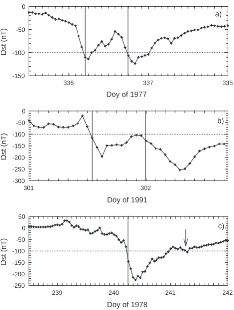
Fig. 1. Dst index for representative events of multiple-step

geo-magnetic storm events with peaks separated more than 12 h, and the corresponding “event time” (solid line): (a) two peaks are well distinguished and theDst index recovers above−100 nT between

both peaks, (b) two peaks are well distinguished, but theDstindex

does not recover above−100 nT between both peaks, and (c) after a former, main peak, and in the last stage of its recovery phase, a second peak appears (indicated with an arrow), which corresponds to a slight decrease below−100 nT and it is not considered as an event. Dotted line in each panel corresponds to the threshold of Dst=−100 nT.

whereD_st∗=Dst−bpPdyn+c, bandcbeing empirical

con-stants and Pdyn solar wind dynamic pressure. Several

au-thors (Fenrich and Luhmann, 1998; O’Brien and McPher-ron, 2000, 2002; C. B. Wang et al., 2003) have considered this model, providing different expressions for the injection function and recovery time (τ).

In this paper, we revise ways of forecasting intense ge-omagnetic activity, taking into account both the Dst peak value or theDst variations. In Sect. 2, we show the state-of-the-art of forecasting with different tools available in the lit-erature. The results indicate that they do not succeed as real-time space weather tools. In Sect. 3, we look for new features in IMF data, and we show how these new features improve the results of the forecasting task. Moreover, only IMF data are involved in this new tool, and forecasting without solar wind density or velocity data is made. In Sect. 4, physical

arguments are presented to explain why the tool works prop-erly. Finally, in Sect. 5, we summarize the conclusions of this study.

2 Analysis of the current warning scenario

To show the scenario of the forecasting task with the tools widely used in literature, we used interplanetary data and Dst data from the OMNIweb database (available at http: //omniweb.gsfc.nasa.gov/). This database provides hourly resolution data from 27 November 1963 to 30 April 2006, although from 1 January 2004, theDst data are provisional. Five-minute resolution interplanetary data are also available for the years 1995 to 2005.

The OMNIweb database comes from several spacecraft (Ace, Wind, IMP8, ISEE3,. . . ) located at different posi-tions. To compare all those datasets, the time provided by this database does not correspond to the time when the mea-surements were done at the spacecraft position but to the time shifted as if the spacecraft were placed on Earth when data were obtained.

2.1 Warning signs of intense magnetic storms

In this section, we show the results in the forecasting task using the criteria from literature for intense storms. Then, setting the aim in the value of theDst peak reached during the storm time (Dstpeak≤−100 nT), we have identified 353 intense storm events from 1963 to 2006, which we are in-terested in forecasting using interplanetary data such as real-time data. Somereal-times, a careful inspection of the experimen-tal data has been necessary in selecting the events, especially in the years of strong geomagnetic activity. Hence, some selection criteria have been established and applied with the aim of making this study valuable not only from the technical point of view but mainly from the scientific one.

Sometimes geomagnetic storms show double or tripleDst peaks (e.g. Kamide et al., 1998). Considering those storm events as unique or multiple events is not an easy task. Our choice has been to consider two different events only ifDst peaks were separated for more than 12 h.

On the other hand, a starting time of theDst event (here-after called “event time”) shall be established with the aim of warning before that time. In the single events, as well as in the cases of multiple-step storms considered as unique events (i.e. with peaks separated less than 12 h), the “event time” is settled at the first time thatDstreaches a value equal or lower than−100 nT. With this criterion, we get the maximum time available to warn of a storm with aDst peak value at least below−100 nT.

other cases, the Dst index is below −100 nT between the peaks (Fig. 1b), considered as different events following the above criterion. In this type of events, the time when the Dstindex starts decreasing again is established as the “event time” for the second one (see Fig. 1b).

Finally, other possible situation is when theDstindex goes below−100 nT a second time (or even more times) after be-ing slightly above this value (Fig. 1c). This feature usually appears in the last stage of the recovery phase of a stronger former storm. In those cases, only the main, former event is considered.

As far as the work with solar wind data is concerned, for determining the warning signs of intense storms, we have used the following criteria separately: (a)Ey≥5 mV/m lasting at least 3 h (Gonzalez and Tsurutani, 1987) and (b) Bz≤−10 nT lasting at least 3 h (Tsurutani and Gonzalez, 1995). Note that, for criterion (a), both solar wind veloc-ity and IMF measurements are needed, whereas for criterion (b), only IMF data are necessary.

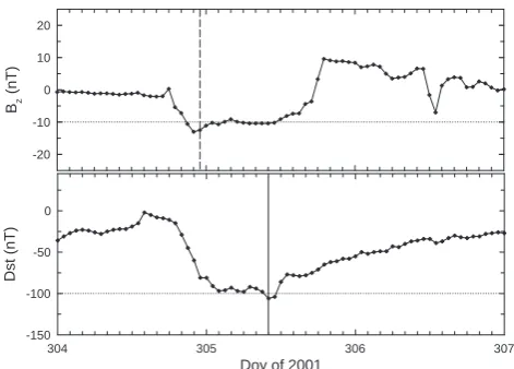
The first time a hazard warning is obtained is called “warn-ing time”. In order to establish an unambiguous relation-ship between this warning and the correspondingDst event, a time interval of 6 h has been considered before and after the “event time”. The choice of this time interval has been done taking into account that: 1) it corresponds to an interval longer enough to comprise the response at terrestrial surface, as measured theDst index, to disturbances coming from the interplanetary medium, 2) it is consistent with the criterion of considering as different events those separated by at least 12 h; a six hours interval between theDst event and that of the warning allows an unambiguous connection, 3) from a statistical point of view, most of the events, throughout the years analyzed, are properly associated within this time in-terval. Nevertheless, in the whole set of events, there are a few for which the “warning time” is more than 6 h in ad-vance. In thoses cases, we have carefully studied the spe-cific event before discarding the association between the in-terplanetary event and the response at terrestrial surface. An example, shown in Fig. 2, is the geomagnetic storm that took place on 1 November 2001 (doy 305). Using criterion (b), a warning takes place on 31 October at 23:00 UT and theDst event starts on 1 November at 10:00 UT. As a consequence, the time interval between “event time” and “warning time” is 11 h, almost twice the time interval selected above. Al-though a technical analysis should tempt us to remove the association between them, from a scientific point of view a cause-effect association seems obvious from Fig. 2.

Once the association of warning events andDst events is concluded, those hazard warning events that are not related to any intense geomagnetic storm event constitute the set of “false alarms”. On the other hand, the warnings have been classified in hits or late warnings, taking into account the value of1t, calculated as the difference between the “event time” and the time of the hazard warning, or “warning time”. This time interval could be considered as the time available

Bz

(nT)

-20 -10 0 10 20

Doy of 2001

304 305 306 307

Dst (nT)

-150 -100 -50 0

Fig. 2.BzandDst index from 31 October (doy 304) to 3

Novem-ber 2001 (doy 307). Dst index is below−100 nT on 1 November

at 10:00 UT (solid line) and a hazard warning takes place first time on 31 October at 23:00 UT (dashed line) using criterion (b). Al-though a difference of 11 h exists between both lines, there is a clear cause-effect association between this interplanetary event and the terrestrial one. Dotted line in top (bottom) panel corresponds to a threshold ofBz=−10 nT (Dst=−100 nT).

to foresee the geomagnetic storm, but, taking into account that interplanetary data have been shifted to the Earth at OM-NIweb database, this1t was only a lower limit of the real available time. Therefore, keeping this idea in mind, we have included every warning with1t≥0 in the set of “hits” (Ta-ble 1). Those events labelled as “late warnings” correspond to events with1t <0. An example of each type of event is shown in Fig. 3, where the dashed vertical line indicates the “warning time” and the solid line indicates the “event time”. Note that, as the time shift from L1 to the Earth depends on the interplanetary shock (or disturbance) propagating speed and the accuracy of the shifting procedure used by the OM-NIweb database, this fact may affect slightly the warning time window.

Finally, the set of “misses” corresponds to those storms with no hazard warning. However, different situations can be distinguished in this set: those events for which criteria (a) or (b) are not fulfilled with interplanetary data available (Fig. 3c), and those where a partial or total data gap in solar wind data does not allow us to conclude the occurrence of a warning. Although both types of events provide the same results for a technical forecasting tool, they should be distin-guished in order to get scientific valuable conclusions.

Bz

(nT)

-40 -20 0 20 40

Doy of 2000

225 226

Dst (nT)

-300 -200 -100 0

(b)

Bz

(nT)

-10 0 10

Doy of 2005

253 254 255 256

Dst (nT)

-200 -150 -100 -50 0

(c) Bz

(nT)

-20 -10 0 10 20

Doy of 2002

131 132 133

Dst (nT)

-150 -100 -50 0

(a)

Fig. 3. Dst index andBz for different scenarios of hazard

warn-ings. Solid (dashed) line in each panel corresponds to “event (warn-ing) time”. From top to bottom the types of event are the follow-ing: (a) Hit: a warning takes place before theDst event, (b) Late

warning: a warning takes place after theDst event, and (c) Miss: a

warning does not exist. Dotted line in top (bottom) panels of each case corresponds to a threshold ofBz=−10 nT (Dst=−100 nT).

in this occasion, just with data from 1998 to 2006. During these years, Ace and Wind spacecraft continuously provided data to the OMNIweb database, at least with the same avail-ability as we have nowadays. The number of events in this case is reduced to 95 events, as can be seen in Table 2, where we show the results for this new set of data. Although there is an improvement from the results of Table 1, up to 48% of hits in case (b), they are still not useful for forecasting purposes. Moreover, none of the 31 misses from Table 2 are related to data gaps before the “event time”. As a con-sequence, these results suggest that some additional effort should be made for a further understanding in solar wind-magnetosphere coupling, leading to a search of complemen-tary features in the solar wind to those proposed by Gonzalez and Tsurutani (1987) and Tsurutani and Gonzalez (1995) for intense geomagnetic activity occurrence.

Table 1. Results of warning of intense storms (Dst peak

≤−100 nT) using the criteria of Gonzalez and Tsurutani (1987) and

Tsurutani and Gonzalez (1995) from 1963 to 2006.

Hits Late warnings False Misses

(1t≥0) (1t <0) alarms

Ey≥5 mV/m 85 (24%) 27 22 241

for1t≥3 h

Bz≤−10 nT 116 (33%) 38 61 199

for1t≥3 h

Table 2. Results of warning of intense storms (Dst peak

≤−100 nT) using the criteria of Gonzalez and Tsurutani (1987) and Tsurutani and Gonzalez (1995) from 1998 to 2006.

Hits Late warnings False Misses

(1t≥0) (1t <0) alarms

Ey≥5 mV/m 39 (41%) 13 4 43

for1t≥3 h

Bz≤−10 nT 46 (48%) 18 17 31

for1t≥3 h

2.2 ForecastingDstvariations (1Dst)

An increase in the rate of space-weather related anomalies and failures related to large variations ofDsthave been iden-tified in recent years. This is the motivation of this section where our aim is to alert of large variations ofDst instead of large Dst values. We will consider that an event takes place at ti if Dst(ti)−Dst(ti−1) is below −50 nT. For this

purpose, we have used again the hourly data from the OMNI-web database from 1963 to 2006, and 100 events have been identified where1Dstwas below−50 nT between two con-secutive data. This set of events, which we are interested in forecasting in order to check our tool, was selected in such a way that it included the most severe geomagnetic storms.

As in Sect. 2.1, in the case of multiple-step storms, our choice has been to consider two different events (in this case 1Dst≤−50 nT) only if they were separated for more than 12 h. We have also classified the results in the forecasting task in the base of the value of1t, calculated as the differ-ence between the time of the event (ti)and the time of the hazard warning.

As is deduced from Eq. (1), a hazard warning should be achieved when 1Dst=Q1t+7.261(pPdyn)≤−50 nT

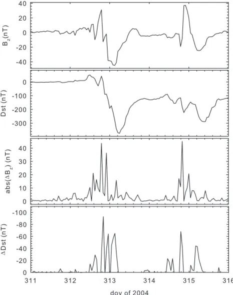
Fig. 4. Geomagnetic activity and interplanetary magnetic field data measured from 7 to 12 November 2004. From top to bottom: Bz,

Dst index, absolute value ofBzhourly variation, andDst hourly

variation (positive values have been omitted in the bottom panel).

al. (1975) and C. B. Wang et al. (2003), after “case of Bur-ton” and “case of Wang”, are used. 13 (16) misses out of those included in Table 3 in the “case of Burton” (“case of Wang”) are not related to data gaps (4 (7) of them after year 1995). Note that the results of both cases are below 35% of hits, which indicate that a forecasting tool based on the above procedures is not trustworthy. Again, the results suggest that other features in the solar wind should be related to the trig-ger of the storm.

3 New warning features

A forecasting tool becomes worthy as far as it is able to give accurate outputs using a minimum number of inputs. During the three most intense geomagnetic storms of the present so-lar cycle, soso-lar wind plasma measurements at L1 presented gaps, but there were no gaps in IMF data. Pallocchia et al. (2006) remarked that plasma instruments can be affected by enhanced solar X-ray and energetic particle fluxes and can fail more often than magnetometers; moreover, sometimes the solar wind speed exceeds the upper instrumental limits of plasma detectors. On the other hand, during these events,

Table 3. Results of warning of events with1Dst≤−50 nT using

the injection function,Q(t ), of Burton et al. (1975) and C. B. Wang et al. (2003) from 1963 to 2006 (see text for details).

Hits Late warnings False Misses

(1t≥0) (1t <0) alarms

Burton et al. (1975) 33 5 28 62

C. B. Wang et al. (2003) 31 4 17 65

Table 4. Results of warning of events with1Dst≤−50 nT using

our model with hourly resolutionBzdata (UAH 1 h).

Hits (1t≥0) Late warnings (1t <0) False alarms Misses

25 12 25 63

a reliableDst forecast is most needed, as such disturbances can be accompanied by very large geomagnetic storms.

Based on this scenario, we have examinedBz data from the OMNIweb database, looking for any feature apart from southward IMF passage that could warn of geomagnetic ac-tivity. Two of the most intense geomagnetic storms of this solar cycle are shown in Fig. 4. TheBz andDst hourly av-erages, together with their hourly variations,1Bzand1Dst, from 7 to 12 November 2004, are shown. One can see thatBz is highly variant at the beginning of both storms, that is, when |1Bz|increases, theDst index decreases. These significant changes inBzhave been found to occur also during interplan-etary shocks or sheaths followed by ICMEs. The relation-ship between these shocks and intense geomagnetic activity is well established in the literature (e.g. Echer and Gonzalez, 2004). Other references related to this significant variation ofBz component can be found in the study of Y. M. Wang et al. (2003), which showed that a compression of a southern Bzcomponent in the shock overtaking a preceding magnetic cloud could increase the geoeffectiveness corresponding to that southern event. In addition, Daglis et al. (2003) pointed out that a major substorm is triggered when a northward turn-ing of the IMF and a dynamic pressure enhancement occur simultaneously during a long interval of southward IMF.

Therefore, we have consideredBzvariations,|1Bz|, over a threshold for a certain time interval as a warning feature for intense geomagnetic activity. We have computed|_1Bz| as the difference between the maximum and the minimum value ofBzin that interval. The best results with 1-h resolu-tion data from OMNIweb are obtained when the threshold for |1Bz|is set at 30 nT and the time interval is 3 h. Therefore, the “warning time” is the corresponding to the third hour of the interval where it takes place.

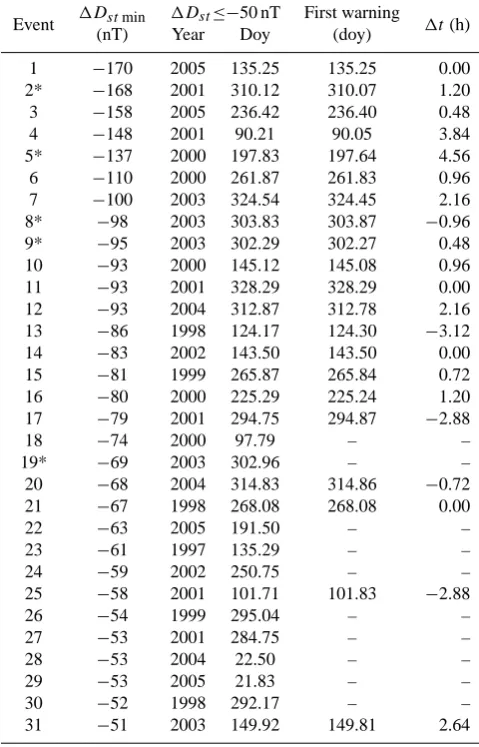
Table 5. Events with1Dst≤−50 nT from 1995 to 2005 and the

warning hazards obtained using our model with 5-min resolution Bzdata (see text for details).

Event 1Dstmin 1Dst≤−50 nT First warning 1t(h)

(nT) Year Doy (doy)

1 −170 2005 135.25 135.25 0.00

2* −168 2001 310.12 310.07 1.20

3 −158 2005 236.42 236.40 0.48

4 −148 2001 90.21 90.05 3.84

5* −137 2000 197.83 197.64 4.56

6 −110 2000 261.87 261.83 0.96

7 −100 2003 324.54 324.45 2.16

8* −98 2003 303.83 303.87 −0.96

9* −95 2003 302.29 302.27 0.48

10 −93 2000 145.12 145.08 0.96

11 −93 2001 328.29 328.29 0.00

12 −93 2004 312.87 312.78 2.16

13 −86 1998 124.17 124.30 −3.12

14 −83 2002 143.50 143.50 0.00

15 −81 1999 265.87 265.84 0.72

16 −80 2000 225.29 225.24 1.20

17 −79 2001 294.75 294.87 −2.88

18 −74 2000 97.79 – –

19* −69 2003 302.96 – –

20 −68 2004 314.83 314.86 −0.72

21 −67 1998 268.08 268.08 0.00

22 −63 2005 191.50 – –

23 −61 1997 135.29 – –

24 −59 2002 250.75 – –

25 −58 2001 101.71 101.83 −2.88

26 −54 1999 295.04 – –

27 −53 2001 284.75 – –

28 −53 2004 22.50 – –

29 −53 2005 21.83 – –

30 −52 1998 292.17 – –

31 −51 2003 149.92 149.81 2.64

results. However, the number of misses has not increased, and the 1t value in late warnings is usually of 1 h, which coincides with the temporal data resolution. Also, the num-ber of false alarms (25) is comparable with that obtained with the Burton injection function (28) but larger than that obtained with the Wang injection function (17). However, included among the 25 “false alarm” events shown in Ta-ble 4 are space weather events such as that of 28 October 1991, when the Qu´ebec-New England DC line tripped out of service, although no event was observed just looking atDst data. This event was neither forecast with the Burton injec-tion funcinjec-tion nor with the Wang one. Furthermore, onlyBz is used as an input in the procedure to obtain our results, in contrast to those of Sect. 2.2, where solar wind density and velocity data were needed to determine the warning hazards.

At this stage, we should not forget that the analysis ofBz variations as a warning feature for intense geomagnetic ac-tivity has been performed using hourly resolution data and the results do not improve too much than those obtained be-fore. However, we should ensure that this choice does not preclude the possible contribution of faster variations in IMF measurements. Then, in order to evaluate the importance of data time resolution, we have analyzed 5-min resolution data from the OMNIweb database. In this case, the period cov-ered was only from January 1995 to December 2005 (there are no data available of this resolution out of this period) and the number of events where 1Dst was below −50 nT per hour was reduced from 100 to 31.

Our warning tool achieves the best results for this 5-min resolution data set with the threshold of|1Bz|set at 44 nT and a time interval of 2.4 h. As expected, the threshold is higher when we improve the temporal resolution.

The set of 31 events (in increasing1Dst order) and the results obtained with our forecasting tool with 5-min reso-lution data are summarized in Table 5. After the number of event (in the 1st column), the second column indicates the minimum value that1Dst reaches for that event. The third and fourth columns indicate the first time (year-doy) that the −50 nT threshold has passed. Note that the minimum1Dst value of column 2 could be reached after the doy of column 4. Doy of the first hazard warning obtained with our tool for every event is included in column 5. A dash at column 5 indicates that our tool does not provide any warning for that event. In that case, that event should be considered as a miss-ing. Finally, in column 6, the hours between the time of the 1Dst event and the corresponding hazard warning appear. As it was explained above, those events with a positive or zero value in column 6 correspond to hits and those with a negative value correspond to late warnings.

A few events, with an asterisk at the 1st column, lacked IMF 5-min resolution data, so we attempted to obtain data from sources other than the OMNIweb database. We found data available from MAG experiments onboard the ACE spacecraft, although some of them still lack solar wind speed data from SWEPAM in ACE and SWE in Wind spacecraft. We averaged the MAG data to obtain the same resolution as the OMNIweb data, 5 min, and we have checked our fore-casting tool with the new data. Then, for the events marked with an asterisk, the results included in Table 5 correspond to ACE data. This fact has to be taken into account because the time delays of column 6 include not only the time between the hazard warning and the event on Earth but also the time shift from L1 to the Earth, which has been considered in the OMNIweb data.

Table 6. Results of warning of events with1Dst≤−50 nT using

our model with 5-min resolutionBzdata (UAH 5 min).

Hits (1t≥0) Late warnings (1t <0) False alarms Misses

16 (52%) 6 6 10

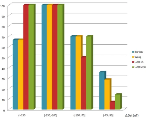
that purpose, we have made four different intervals of1Dst and we have analyzed the number of hits in each interval for years 1995–2005. The intervals are the following: (a) 1Dst≤−150 nT, (b) −150 nT<1Dst≤−100 nT, (c) −100 nT<1Dst≤−75 nT, and (d) −75 nT <1Dst≤−50 nT. Then, we have checked the hits with every tool explained above to forecast1Dst: with Burton et al. (1975) and C. B. Wang et al. (2003) injection functions, with hourly resolution data, and with our tool (UAH) with hourly and 5-min resolution data. It is not possible to use 5-min resolution data in the cases of Burton and Wang because, in both cases, the injection function is an empirical function obtained from hourly resolution data, and then, it will not be appropriate to use it with other resolution data. However, we have selected the same data range (1995–2005) for every tool in order to compare. Figure 5 shows clearly the high quality of our tool forecasting for largeDst variation events, when 5-min resolution data are used as real-time data, even for those events without plasma data available at L1. This excellent behavior disappears in our tool when we are trying to forecast smallDst variations, while other tools are able to foresee about 30% of the events. Nevertheless, it should be noted that the events set for intervals (a) and (b) are relatively small (3 and 4 events, respectively) and further investigations are needed to confirm this outstanding result when upcoming data are available.

4 Discussion

The immediate goal of the reported research is to develop a 1Dstforecasting tool based only onBzdata measured at L1, which let us improve the present scenario, where the lack of plasma data does not allow one to make trustworthy predic-tions during the most severe geomagnetic storms. We have shown in Sect. 3 the reliability of this tool in forecasting se-vere1Dst. This application guides us to make new propos-als in the physical processes involved in the main phase of geomagnetic storms.

In the present scenario, when IMF presents a large and long-duration southern component, the energy supplied from solar wind to the inner magnetosphere is more effective as a consequence of reconnection. Equation (1) assumes that, when reconnection takes place, the convective electric field

Fig. 5. Results of warning1Dst≤−50 nT as a function of the1Dst

using different tools explained in the text: (a) with the injection function,Q(t ), of Burton et al. (1975); (b) with the injection func-tion of C. B. Wang et al. (2003), (c) with our tool applied to hourly resolutionBzdata (UAH 1 h), and (d) with our tool applied to 5-min

resolutionBzdata (UAH 5 min). Vertical axis indicates the

percent-age of hits for each1Dst interval. For comparison purposes, only

results from years 1995 to 2005 are shown in the graph.

penetrates into the magnetosphere, injecting particles to the inner magnetosphere.

A simple description of the electric field of the magne-totail in the equatorial plane of the magnetosphere is given by the Volland-Stern electric potential (Volland, 1973; Stern, 1975). On the other hand, convective electric field can be also expressed as a function of cap polar potential (Boyle et al., 1997). Both electric potential models lead to a large-scale potential structure of the magnetosphere, where the electric field in the magnetotail follows the dawn-dusk direc-tion, and drives particles from the tail to the inner magneto-sphere. Simplified assumptions about electric and magnetic field are done, but they are not enough to consider the large variety of phenomena that take place in the development of a geomagnetic storm.

The electric field satisfies Faraday’s law, which general ex-pression is given by the following equation:

∇ ×E= ∇ ×(v×B)−∂B

∂t (2)

The first term on the right side corresponds to the contri-bution to the electric field due to the motion of solar wind plasma (convective electric field). The second term corre-sponds to the explicit temporal variation of IMF. Usually, in order to consider stationary convection, this last term does not appear. This seems a reasonable approach, taking into account that explicit variations of magnetic field vec-tor are only significant from time to time. Then, the effect of IMF temporal variations, within observational uncertain-ties, is unnoticed in procedures involving long-period data series, as those used in Burton et al. (1975) and C. B. Wang et al. (2003). Subsequently, it is possible for many purposes to consider the source of electric field as if it were only due to the term related to the motion of plasma. However, it could be not appropriate if we are interested in the main phases of severe geomagnetic storms. During these periods, the instru-ments on board of spacecraft located at L1 are used to mea-sure highly fluctuating IMF, related to interplanetary shocks and sheaths preceding magnetic clouds or corotating inter-action regions, and then, the last term in Eq. (2) cannot be ignored.

To analyze only the dawn-dusk component in Eq. (2), it is convenient to use the vector potential,A, instead of magnetic field vector,B, so that

∇ ×E= ∇ ×(v×B)− ∂

∂t(∇ ×A) (3)

Therefore,

E=(v×B)−∂A

∂t (4)

Assuming, as a first approach, that onlyBzis involved in the effective solar wind-magnetosphere coupling and taking into account that the solar wind velocity can be approached by its Sun-Earth component, Eq. (4) enables one to determine the dawn-dusk electric field (Ey)as follows

Ey =vxBz− ∂Ay

∂t (5)

and bothvxBzand ∂Ay

∂t are involved in the calculation ofEy. Theycomponent of potential vector,Ay, is related to the x andzcomponents of IMF. But, assuming as above men-tioned, that onlyBz is involved in the coupling between so-lar wind and magnetosphere, it is possible to approach the dawn-dusk electric field as the addition of two contributions: the convective electric field (vxBz) and a function of ∂B_∂tz. The knowledge of the function which relatesAyand ∂B_∂tz is an unavoidable task before discussing about the significance of the rate of change inBz relative to the convective elec-tric field in Eq. (5). However, the empirical results of Sect. 3

indicate that|1Bz|of 44 nT in1t=2.4 h will cause in terres-trial surface a1Dst≤−50 nT in one hour. On the other hand, in the present scenario, to calculate an equivalent decrease on Dst caused by the convective electric field, it will be deduce from the expression1Dst=Q1t+7.261 pPdyn, as stated

in Sect. 2.2. Neglecting pressure effects and considering the Burton injection function,1Dst≤−50 nT in one hour will be caused by a VBs≥50/5.4 mV/m, withBs=|Bz|for southern Bzand zero otherwise. Thus it is important to point out that a rate of change inBzof 5×10−3nT/s and a convective elec-tric field of 9.26 mV/m could produce equivalent response of the ring current.

Usually, both contributions toEy from Eq. (5) appear in solar wind and it is difficult to separate how much each one contributes to the ring current disturbance. Moreover, com-paring events with similar convective electric field values and similar values of|_1Bz|in a time interval of 2.4 h,1Dst in one hour does not reach the same value. As an example, we can refer to the events 4 and 12 (Table 5) with1Dstminof −148 and−93 nT in one hour, respectively. The explanation could be related to solar wind dynamic pressure, which has been proved to be an important factor to enhance the intensity of large storms (Xie et al., 2008).

A separate analysis of three contributions involved inDst index (convective electric field, temporal variations ofBzand dynamic pressure) is not an easy task. From the beginning, studies aboutDstindex have considered that solar wind pres-sure was involved in this index. However, this parameter was soon included in the injection function to calculate the so-called “pressure corrected”Dst. Moreover, recent papers (Xie et al., 2008) obtain an expression for dynamic pressure corrections of Dst index depending on convective electric field. Thus, from previous works, it can be concluded that different contributions toDst are not independent and some coupled terms should be considered inDstcomputation from solar wind data. As a result, the expression to determineDst from solar wind parameters is not just an addition of three separate functions of VBs,1Bz

1tandPdyn. A future work

will be dedicated to this task. Nevertheless, all we can de-duce from our results is that there will be energy release from solar wind to terrestrial magnetosphere when a dawn-dusk electric field arises. But, to calculate this electric field, it is necessary to take into account not only the convective term (as it is usually considered) but also to add a function which depends on temporal variations ofBz.

5 Summary and conclusions

value and (2) hourly variation. The results let us conclude that the above features in electric or magnetic field could forecast less than 50% of impending intense storms (peak Dst≤−100 nT). Moreover, only about 33% of events with 1Dst below−50 nT were predicted on time in the case of Burton and only 31% in the case of Wang. In both cases, the number of false alarms was somewhat similar and compara-ble with the number of hits in the case of Burton.

Previous results guided us in looking for new features in solar wind data that could forecast intense geomagnetic ac-tivity. Variations ofBz over a threshold for a certain time interval succeeded in warning of largeDsthourly variations. We analyzed the success of this forecasting tool with two different sets of data: hourly (1963–2006) and 5-min (1995– 2005) resolution data from the OMNIweb database. The re-sults improved with the highest resolution data for large vari-ation ofDst but are worse than previous models for small variations of that index. Moreover, although the results are not shown, as a general case, the times from the hazard warn-ing until the event happens on Earth have been improved with our tool relative to other tools implemented in this paper.

The new view of solar wind-magnetosphere interaction is explained on the basis of Faraday’s law, discussing how not only southern IMF but also large and fast temporal variations of interplanetary magnetic field could develop intense dawn-dusk electric field. This scenario provides a general view of the effect of IMF on the magnetosphere, where both, move-ment and variations of IMF, contribute to the enhancemove-ment of the ring current.

In conclusion, we found that large variations in theDst in-dex are related not only to southernBzbut also to significant temporal variations inBz. As a consequence, the develop-ment of severe geomagnetic storms seems to be related only toBz, and then, solar wind velocity seemingly does not play any role. However, experimental data show that large tem-poral IMF variations take place in shocks and sheaths, which arise as a consequence of the interaction of a fast solar wind and the ambient one.

Trying to get light in the solar wind-magnetosphere inter-action, the scenario could be summarized as follows:

1. There will be energy transfer from solar wind to mag-netosphere, not only because of the arrival of a southern interplanetary magnetic field at the nose of the magne-topause, and via reconnection a subsequent large-scale convection towards the tail, but also because of fluctua-tions in z-component of IMF.

2. In order to quantify the energy transferred from solar wind to magnetosphere from the two contributions men-tioned in 1), the expression for the first case depends ex-plicitly on both,Bzand solar wind velocity, while in the second one solar wind velocity is not involved.

3. As fluctuation in Bz seems to be a precursor of large Dstvariations in the main phase of intense geomagnetic

storms, it is possible to alert only with Bz, although other solar wind parameters could be involved in the task of forecasting the intensity of the storm.

Therefore, we consider our results useful not only in fore-casting space weather task but also for upcoming models of solar wind-magnetosphere interaction. Particle flux measure-ments from the ring current and their relationship to the dif-ferent contributions of dawn-dusk electric field will be stud-ied in a future work. We are also interested in obtaining a theoretical expression for the function related to the tempo-ral variation of the zcomponent of IMF and to extend the present study to higher resolution data sets.

Acknowledgements. We thank the Space Physics Data Facility and OMNIweb service for theDst index and solar wind data. We are

also grateful to the ACE MAG instrument team and the ACE Sci-ence Center for the magnetic field data. This work has been sup-ported by grants from the Comisi´on Interministerial de Ciencia y Tecnolog´ıa (CICYT) of Spain (ESP 2005-07290-C02-01 and ESP 2006-08459).

Topical Editor I. A. Daglis thanks Y. Kamide and another anony-mous referee for their help in evaluating this paper.

References

Boyle, C. B., Reiff, P. H., and Hairston, M. R.: Empirical polar cap potentials, J. Geophys. Res., 102, 111–126, 1997.

Brueckner, G. E., Delaboudiniere, J. P., Howard, R. A., Paswaters, S. E., Cyr, O. C. St., Schwenn, R., Lamy, P. L., Simnett, G. M., Thompson, B., and Wang, D.: Geomagnetic storms caused by coronal mass ejections (CMEs): March 1996 through June 1997, Geophys. Res. Lett., 25, 3019–3022, 1998.

Burton, R. K., McPherron, R. L., and Russell, C. T.: An empirical relationship between interplanetary conditions andDst, J.

Geo-phys. Res., 80, 4204–4214, 1975.

Cane, H. V., Richardson, I. G., and Cyr, O. C. St.: Coronal mass ejections, interplanetary ejecta and geomagnetic storms, Geo-phys. Res. Lett., 27, 3591–3594, 2000.

Cid, C., Hidalgo, M. A., Saiz, E., Cerrato, Y., and Sequeiros, J.: Sources of intense geomagnetic storms over the rise of solar cy-cle 23, Solar Phys., 223, 231–243, 2004.

Daglis, I. A., Kozyra, J. U., Kamide, Y., Vassiliadis, D., Sharma, A. S., Liemohn, M. W., Gonzalez, W. D., Tsurutani, B. T., and Lu G.: Intense space storms: Critical issues and open disputes, J. Geophys. Res., 108(A5), 1208, doi:10.1029/2002JA009722, 2003.

Echer, E. and Gonzalez, W. D.: Geoeffectiveness of interplan-etary shocks, magnetic clouds, sector boundary crossings and their combined occurrence, Geophys. Res. Lett., 31, L09808, doi:10.1029/2003GL019199, 2004.

Echer, E., Alves, M. V., and Gonzalez, W. D.: A statistical study of magnetic cloud parameters and geoeffectiveness, J. Atmos. Terr. Phys., 67, 839–852, 2005.

Gonzalez, W. D. and Tsurutani, B. T.: Criteria of interplanetary parameters causing intense magnetic storms (Dst<−100 nT),

Planet. Space Sci., 35, 1101–1109, 1987.

Gonzalez, W. D., Echer, E., Clua-Gonzalez, A. L., and Tsuru-tani, B. T.: Interplanetary origin of intense geomagnetic storms (Dst<−100 nT) during solar cycle 23, Geophys. Res. Lett., 34,

L06101, doi:10.1029/2006GL028879, 2007.

Gopalswamy, N., Lara, A., Lepping, R. P., Kaiser, M. L., Berdichevsky, D., and Cyr, O. C. St.: Interplanetary accelera-tion of coronal mass ejecaccelera-tions, Geophys. Res. Lett., 27, 145–148, 2000.

Gopalswamy, N., Yashiro, S., Michalek, G., Xie, H., Lepping, P. R., and Howard, R. A.: Solar source of the largest geo-magnetic storm of cycle 23, Geophys. Res. Lett., 32, L12S09, doi:10.1029/2004GL021639, 2005.

Gosling, J. T., McComas, D. J., Phillips, J. L., and Bame, S. J.: Geo-magnetic activity associated with Earth passage of interplanetary shock disturbances and coronal mass ejections, J. Geophys. Res., 96, 7831–7839, 1991.

Huttunen, K. E. J., Koskinen, H. E. J., Pulkkinen, T. I., Pulkkinen, A., Palmroth, M., Reeves, E. G. D., and Singer, H. J.: April 2000 magnetic storm: Solar wind driver and magnetospheric response, J. Geophys. Res., 107(A12), 1440, doi:10.1029/2001JA009154, 2002.

Kamide, Y., Yokoyama, N., Gonzalez, W. D., Tsurutani, B. T., Daglis, I. A., Brekke, A., and Masuda, S.: Two-step develop-ment of geomagnetic storms, J. Geophys. Res., 103, 6917–6921, 1998.

Kamide, Y.: Interplanetary and magnetospheric electric fields dur-ing geomagnetic storms: What is more important, steady-state fields or fluctuating fields?, J. Atmos. Solar-Terr. Phys., 63, 413– 420, 2001.

Kokubun, S., McPherron, R. L., and Russell, C. T.: Triggering of substorms by solar wind discontinuities, J. Geophys. Res., 82, 74–86, 1977.

O’Brien, T. P. and McPherron, R. L.: An empirical phase-space analysis of ring current dynamics: solar wind control of injection and decay, J. Geophys. Res., 105, 7707–7720, 2000.

O’Brien, T. P., McPherron, R. L., and Liemohn, M. W.: Continued convection and the initial recovery ofDst, Geophys. Res. Lett.,

29(23), 2143, doi:10.1029/2002GL015556, 2002.

Pallocchia, G., Amata, E., Consolini, G., Marcucci, M. F., and Bertello, I.: GeomagneticDst index forecast based on IMF data

only, Ann. Geophys., 24, 989–999, 2006, http://www.ann-geophys.net/24/989/2006/.

Pulkkinen, T.: Space Weather: Terrestrial Perspective, Living Rev. Solar Phys, 4, 1 p., available at: http://solarphysics. livingreviews.org/Articles/lrsp-2007-1/, 2007.

Richardson, I. G., Cane, H. V., and Cliver, E. W.: Sources of geo-magnetic activity during nearly three solar cycles (1972–2000), J. Geophys. Res., 107(A8), 1187, doi:10.1029/2001JA000504, 2002.

Richardson, I. G., Webb, D. F., Zhang, J., Berdichevsky, D. B., Biesecker, D. A., Kasper, J. C., Kataoka, R., Steinberg, J. T., Thompson, B. J., Wu, C. C., and Zhukov, A. N.: Ma-jor geomagnetic storms (Dst≤−100 nT) generated by

coro-tating interaction regions, J. Geophys. Res., 111, A07S09, doi:10.1029/2005JA011476, 2006.

Stern, D. P.: The motion of a proton in the equatorial magneto-sphere, J. Geophys. Res., 80, 595–599, 1975.

Tsurutani, B. T.: The interplanetary causes of magnetic storms, substorms and geomagnetic quiet in Space Storms and Space Weather Hazards, edited by: Daglis, I. A., 103, Kluwer Aca-demic Press, Norwell, 2001.

Tsurutani, B. T. and Gonzalez, W. D.: The future of geomagnetic storm predictions: Implications from recent solar and interplan-etary observations, J. Atmos. Solar Terr. Phys., 57, 1369–1384, 1995.

Volland, H.: Semiempirical model of large-scale magnetospheric electric field, J. Geophys. Res., 78, 171–180, 1973.

Wang, Y. M., Ye, P. Z., Wang, S., Zhou, G. P., and Wang, J. X.: Sta-tistical study on the geoeffectiveness of Earth-directed coronal mass ejections from March 1997 to December 2000, J. Geophys. Res., 107(A11) 1340, doi:101029/2002JA009244, 2002. Wang, C. B., Chao, J. K., and Lin, C. H.: Influence of the solar wind

dynamic pressure on the decay and injection of the ring current, J. Geophys. Res., 108(A9) 1341, doi:10.129/2003JA009851, 2003.

Wang, Y. M., Ye, P. Z., Wang, S., and Xue, X. H.: An interplanetary cause of large geomagnetic storms: Fast forward shock overtak-ing precedovertak-ing magnetic cloud, Geophys. Res. Lett., 30(13), 1700, doi:10.1029/2002GL016861, 2003.

Webb, D. F., Cliver, E. W., Crooker, N. U., Cyr, O. C. St., and Thompson, B. J.: Relationship of halo coronal mass ejections, magnetic clouds, and magnetic storms, J. Geophys. Res., 105, 7491–7508, 2000.

Xie, H., Gopalswamy, N., Cyr, O. C. St., and Yashiro, S.: Ef-fects of solar wind dynamic pressure and preconditioning on large geomagnetic storms, Geophys. Res. Lett., 35, L06S08, doi:10.1029/2007GL032298, 2008.

Zhang, J., Dere, K., Howard, R. A., and Bothmer, V.: Identification of solar sources of major geomagnetic storms between 1996 and 2000, Astrophys. J., 582, 520–533, 2003.