Dynamics of thin current sheets: Cluster observations

www.ann-geophys.net/25/1365/2007/ © European Geosciences Union 2007

Annales

Geophysicae

Dynamics of thin current sheets: Cluster observations

W. Baumjohann1, A. Roux2, O. Le Contel2, R. Nakamura1, J. Birn3, M. Hoshino4, A. T. Y. Lui5, C. J. Owen6, J.-A. Sauvaud7, A. Vaivads8, D. Fontaine2, and A. Runov1

1_{Space Research Institute, Austrian Academy of Sciences, Graz, Austria} 2_{CETP-IPSL-CNRS, V´elizy, France}

3_{Los Alamos National Laboratory, Los Alamos, NM, USA} 4_{University of Tokyo, Tokyo, Japan}

5_{JHU/APL, Laurel, MD, USA}

6_{Mullard Space Science Laboratory, Univ. College London, UK} 7_{CESR/CNRS, Toulouse, France}

8_{Swedish Institute of Space Physics, Uppsala, Sweden}

Received: 25 January 2007 – Accepted: 24 May 2007 – Published: 29 June 2007

Abstract. The paper tries to sort out the specific signatures of the Near Earth Neutral Line (NENL) and the Current Dis-ruption (CD) models, and looks for these signatures in Clus-ter data from two events. For both events transient mag-netic signatures are observed, together with fast ion flows. In the simplest form of NENL scenario, with a large-scale two-dimensional reconnection site, quasi-invariance along Y is expected. Thus the magnetic signatures in the S/C frame are interpreted as relative motions, along the X or Z direc-tion, of a quasi-steady X-line, with respect to the S/C. In the simplest form of CD scenario an azimuthal modulation is expected. Hence the signatures in the S/C frame are in-terpreted as signatures of azimuthally (along Y) moving cur-rent system associated with low frequency fluctuations ofJy

and the corresponding field-aligned currents (Jx). Event 1

covers a pseudo-breakup, developing only at high latitudes. First, a thin (H≈2000 km≈2ρi, withρi the ion gyroradius)

Current Sheet (CS) is found to be quiet. A slightly thinner CS (H≈1000–2000 km≈1–2ρi), crossed about 30 min later,

is found to be active, with fast earthward ion flow bursts (300–600 km/s) and simultaneous large amplitude fluctua-tions (δB/B∼1). In the quiet CS the current densityJy is

carried by ions. Conversely, in the active CS ions are mov-ing eastward; the westward current is carried by electrons that move eastward, faster than ions. Similarly, the veloc-ity of earthward flows (300–600 km/s), observed during the active period, maximizes near or at the CS center. During the active phase of Event 1 no signature of the crossing of an X-line is identified, but an X-line located beyond Clus-ter could account for the observed ion flows, provided that it is active for at least 20 min. Ion flow bursts can also be

Correspondence to: W. Baumjohann

(baumjohann@oeaw.ac.at)

due to CD and to the corresponding dipolarizations which are associated with changes in the current density. Yet their durations are shorter than the duration of the active period. While the overall∂Bz/∂tis too weak to accelerate ions up to

the observed velocities, short duration∂Bz/∂t can produce

the azimuthal electric field requested to account for the ob-served ion flow bursts. The corresponding large amplitude perturbations are shown to move eastward, which suggests that the reduction in the tail current could be achieved via a series of eastward traveling partial dipolarisations/CD. The second event is much more active than the first one. The observed flapping of the CS corresponds to an azimuthally propagating wave. A reversal in the proton flow velocity, from −1000 to +1000 km/s, is measured by CODIF. The overall flow reversal, the associated change in the sign of

Bzand the relationship betweenBx andBysuggest that the

spacecraft are moving with respect to an X-line and its asso-ciated Hall-structure. Yet, a simple tailward retreat of a large-scale X-line cannot account for all the observations, since several flow reversals are observed. These quasi-periodic flow reversals can also be associated with an azimuthal mo-tion of the low frequency oscillamo-tions. Indeed, at the begin-ning of the intervalBy varies rapidly along the Y direction;

the magnetic signature is three-dimensional and essentially corresponds to a structure of filamentary field-aligned cur-rent, moving eastward at∼200 km/s. The transverse size of the structure is∼1000 km. Similar structures are observed before and after. These filamentary structures are consistent with an eastward propagation of an azimuthal modulation as-sociated with a current systemJy,Jx. During Event 1,

signa-tures of filamentary field-aligned current strucsigna-tures are also observed, in association with modulations ofJy. Hence, for

Keywords. Magnetospheric physics (Magnetotail; Plasma sheet) – Space plasma physics (Plasma waves and instabil-ities; Magnetic reconnection)

1 Introduction

Sudden releases of large amounts of magnetic energy, pre-sumably due to plasma instabilities, occur during magneto-spheric substorms. The plasma confinement is lost over a short time interval, while electrons and ions are accelerated, heated, and precipitated onto the upper atmosphere, which leads to the formation of auroras. Before this rapid heat-ing/acceleration phase, the magnetic energy is slowly accu-mulated in the system, which leads to the formation of thin current sheets. Thus the quasi-steady formation of a thin cur-rent sheet seems to be a necessary step, whereby the con-ditions for an explosive release of magnetic energy are be-ing set up. While this sequence of events is relatively well documented, thanks to numerous in-situ and remote sens-ing observations, there is no consensus yet about the pro-cess(es) that trigger(s) substorms. At the present time, two main scenarios are considered for magnetotail activity rele-vant for substorms. Large-scale MHD simulations of tail dy-namics (Birn and Hesse, 1991, 1996; Hesse and Birn, 1991; Scholer and Otto, 1991; Birn et al., 1999) suggest that both plasmoid ejection and current reduction and diversion, de-scribed as the substorm current wedge (e.g. McPherron et al., 1973) are initiated by the formation of an X-line, causing both tailward and earthward plasma flow. The braking of the earthward flow in the inner tail leads to pile-up of magnetic flux and hence a dipolarization of the magnetic field (Hesse and Birn, 1991; Shiokawa et al., 1997; Baumjohann et al., 1999; Baumjohann, 2002) the diversion of the flow and the associated shear distort the magnetic field and build up the field-aligned currents of the substorm current wedge. This model is commonly referred to as the “near-Earth neutral line model” (Baker et al., 1996).

An alternative scenario, usually called “current disruption model,” assumes that a substorm is triggered locally in the in-ner magnetotail, presumably by an instability that involves a cross-tail wave vector component (Lui, 1991). Potential can-didates are cross-field current-driven instabilities (e.g. Lui, 1991) or interchange/ballooning modes (Roux et al., 1991; Hurricane et al., 1997; Pu et al., 1997; Bhattacharjee et al., 1998a,b; Cheng and Lui, 1998). The disruption of the per-pendicular current can also be due to the interruption of the parallel current by an instability (Perraut et al., 2000). In the current disruption scenario, the formation of an X-line might be a later consequence of the dynamic evolution (Lui, 1996). In order to resolve at least part of the “substorm contro-versy”, theorists as well as data analysts, formed a “Sub-storm Onset Physics” team, that met twice at the Interna-tional Space Science Institute in Bern, Switzerland. The team

aimed at using data from the Cluster mission to discern be-tween the two competing models. After some discussion, it was decided to focus on one of the key differences between the two models: the distinction between the waves that per-turb the thin current sheet at substorm onset and their role in initiating the onset. The neutral line model is characterized by variations along the tail axis, whereas current disruption models are based on modes propagating azimuthally, i.e. par-allel or antiparpar-allel to the cross-tail current.

Hence, the team selected three periods when the Cluster spacecraft observed thin current sheet. Three intervals can give three examples only, but they were selected to cover a quiet thin current sheet, a thin current sheet during a weak substorm, and a thin current sheet during a storm-time sub-storm, and are thus thought to be representative for typical magnetospheric conditions.

2 Models and signatures

From the data which will be presented in Sects. 3 and 4 it will be clear that thin current sheets can be present in the magne-totail under a variety of conditions, ranging from relatively quiet through modestly active to very active, strongly driven scenarios. Accordingly we will discuss here relevant theories and modeling results including quasi-static models as well as instabilities related to thin current sheets.

In the following sections we will first present some major results from quasi-static models, then address details and im-plications of the near-Earth neutral line scenario and finally of the current disruption model(s). These models are not mu-tually exclusive. Rather, they may apply simultaneously, for instance, a relatively quiet, quasi-static, structure may exist within a propagating wave mode. Or they may be causally related; for instance, a small-scale wave mode may be nec-essary to provide the dissipation necnec-essary for a large-scale mode, or the large-scale mode may lead to flows that become turbulent and thus drive smaller scale modes or modes with different wave vectors. A major distinction between the two substorm scenarios detailed in the Introduction is not whether current disruption occurs in one but not the other, but rather whether the responsible mode vectors are primarily in the X direction, along the tail, as in the simplest reconnection sce-nario, or in the y direction, across the tail, as in the simplest current disruption models. However, as indicated above, this distinction also may be an oversimplification. Further, as dis-cussed below, negativeBzvalues, generally thought to be the

-6 -4 -2 0 2 4 6 J

z 0

1 2 3

J tot

J_i

J_e

-6 -4 -2 0 2 4 6

J

z 0

1 2

-4 -3 -2 -1 0 1 2 3 4

J

z 0

1 0.5 1.0

ρ

i=1

ρ

i=0.1

ρ

i=0.01

Fig. 1. Ion (green) and electron (red) contributions to the total

cur-rent (black) in self-consistent models of a thin curcur-rent sheet embed-ded in a wider current sheet, for various ion gyroradii scaled by the half-thickness of the wide current sheet; modified after Schindler and Birn (2002).

2.1 Quasi-equilibrium models

Quasi-static thin current sheet structures in the magnetotail may arise from the response to deformations imposed by the solar wind (Birn and Schindler, 2002). Both MHD and par-ticle simulations consistently demonstrate that a thin current sheet can form as the consequence of the addition of mag-netic flux to the lobes (Schindler and Birn, 1993; Pritchett and Coroniti, 1994; Hesse et al., 1996) An important role is played by the variation inX, the Earth-Sun direction (Birn et al., 1998). Quasi one-dimensional compression leads only to a moderate current density increase. However, a finite, not necessarily short-scale, variation inX can produce a local current density enhancement that is much stronger. Particle and MHD simulations show qualitatively similar behavior, but kinetic effects modify the current sheet structure when the thickness approaches, or becomes less than, a typical ion

z

y

E

v

B

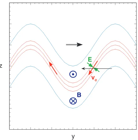
Fig. 2. Thin current sheet embedded in a wider current sheet which

undergoes a kink mode propagating in y, as indicated by the double arrow. The red arrow indicates the fast electron drift in the em-bedded current sheet. The green arrows indicate the electric field associated with that drift. The blue circles with a cross and a dot, respectively, show the magnetic field direction, and the single black arrow indicates the motion of the Cluster satellites relative to the moving structure.

gyroradius, as defined by the field strength outside the cur-rent sheet. Such thin sheets have actually been detected by Cluster (e.g., Nakamura et al., 2002, 2006a).

Recently, Schindler and Birn (2002) derived self-consistent models of thin current sheets embedded within a wider plasma/current sheet. These models are solutions to the Vlasov equations of collisionless plasmas. They can hence serve to illustrate the changes in structure and the con-tributions to the currents under various scales. Two main re-sults are of relevance here.

When the thickness of the current sheet becomes compa-rable to, or smaller than, a typical ion gyroradius or ion in-ertia length, the ion contribution to the thin current sheet is smeared out, so that the current in the thin sheet becomes dominated by the electrons. This is illustrated by Fig. 1, which shows the current contributions in thin embedded cur-rent sheets for 3 values of the ion gyroradius, scaled by the width of the wider current sheet.

Self-consistent equilibrium solutions generally require an electrostatic potential. For two-dimensional configurations withEy=0, when the ion and electron distributions are

func-tions of the total energy and the canonical momentumPy,

Fig. 3. Ion and electron flow velocity vectors in the x, z plane obtained in a particle-in-cell simulation of collisionless magnetic reconnection by Hoshino et al. (2001). The lengths of velocity vec-tors are normalized by the initial ion and electron thermal speed, re-spectively. The bottom panels show electron velocity distributions obtained at the indicated locations.

and Birn, 2002). The value of the electrostatic potential, however, depends on the working frame. In the case of the Harris sheet the electrostatic potential is zero in a frame in which the electric field outside the current sheet vanishes, but in another frame a finite electrostatic potential is requested to ensure quasi-neutrality. TheE×Bdrift of electrons in the electric field corresponding to a thin embedded current sheet (not shared by the ions for thin sheets) can carry the electric current associated with the thin sheet. In a locally planar, one-dimensional model, the electric field is directed towards the centre of the current sheet (Z direction), while a tilt or a corrugation of the current sheet through kink modes, as recently observed by the Cluster and Geotail satellites (e.g. Zhang et al., 2002; Sergeev et al., 2003, 2004, 2006), would generate an additional y component of the electric field, as illustrated in Fig. 2.

2.2 Magnetic tearing or reconnection, kinetic models The understanding of the physics of collisionless magnetic reconnection and of the (two-dimensional) field structure in the vicinity of the reconnection site has increased

consider-ably over the years from a large number of simulations (e.g. Hewett et al., 1988; Pritchett, 1994, 2001; Tanaka, 1995a,b; Hesse et al., 1995, 1999, 2001a; Hesse and Winske, 1998). In the following we will discuss the current sheet structure expected from the magnetic reconnection model, based on particle-in-cell simulation results by Hoshino et al. (2001).

Figure 3 shows ion (top) and electron (bottom) velocity vectors in theXZ plane, together with four electron distri-bution functions. The magnitudes of the ion and electron flow vectors are normalized by the initial ion and electron thermal velocity, respectively. The ion flows are basically directed from the X-type region to the O-type region, and the electron flow is also in the same direction in the plasma sheet. In the outflow region (|X|>6), both ions and electrons have the same bulk velocity of 0.6Vt hi or∼0.5VA, where

Vt hi andVA are the ion thermal and the Alfv´en speeds,

re-spectively. Inside that region the ions are unmagnetized and ion and electron flow speeds differ (“Hall region”). There is “cold” electron flow near the outer boundary between the lobe and the plasma sheet, directed toward the X-type region, and outward electron flow inside this boundary, which con-sists of two populations of “cold” electrons and “hot” elec-tron beams. These flows are associated with Hall electric currents in a thin plasma sheet with a thickness of the order of the ion inertia length.

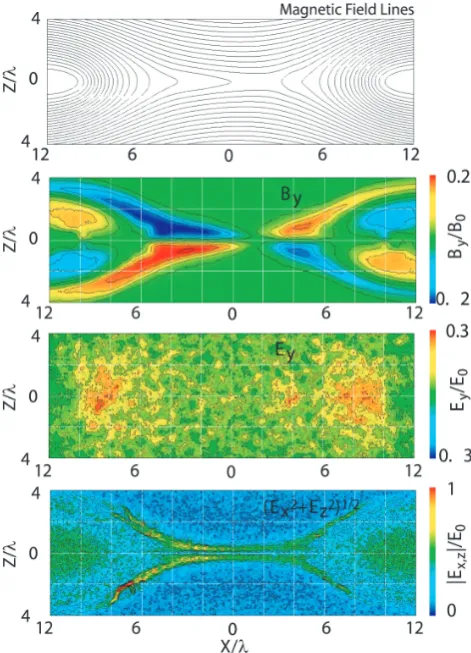
Inside the ion diffusion region near the X-type point where the ions are unmagnetized, the electron flow becomes faster than the ion flow. The magnetized electrons can have a largeE×B drift velocity in a weak magnetic field region, which can become larger than the Alfv´en velocity. This rel-ative flow difference between ions and electrons produces Hall currents in the reconnection plane, corresponding to quadrupolar dawn- dusk magnetic fields as shown in the sec-ond panel of Fig. 4. Maintaining the continuity of the elec-tric current, a field-aligned elecelec-tric current is generated in the outer boundary, associated with field-aligned electron mo-tion. The dawn-dusk electric fieldEy is positive in the

re-connection region, and the strongest electric fieldEyis found

between the X-type region and the O-type region. In addition to the global reconnection electric field, a small scale, bursty electric field structure can also be found. In the bottom panel, the amplitude of the electric fields in the reconnection plane,

|Ex,z|=

q E2

x+E2z, is depicted. The strongest intensity can

be found in the quadrupolarBy region (i.e. the Hall electric

current region), whose thickness is of the order of ion iner-tia length. The polarization electric field toward the neutral sheet is produced by the inertia difference between ions and electrons across the boundary. In addition to the large-scale X-type structure ofEx,z, a small-scale structure embedded

While the two-dimensional structure of the reconnection site appears well understood, the structure in the cross-tail direction is less well explored. Due to the complex-ity of the problem and the numerical effort involved, only a few three-dimensional simulations of collisionless recon-nection have been performed (e.g., Tanaka, 1995a; Pritchett and Coroniti, 1996). As a result, the question of whether the results from 2.5-dimensional models carry over to more realistic, three-dimensional configurations remains largely open. Recent three-dimensional simulations (Rogers et al., 2000; Hesse et al., 2001b; Zeiler et al., 2002) support the view that collisionless magnetic reconnection in 3-D current sheets operates in a manner very similar to the results de-rived from translationally invariant models. The develop-ment of structure in the out-of-plane direction appears to be limited to small scales which may enhance local dissipation coefficients (Huba et al., 1978; B¨uchner, 1998; B¨uchner and Kuska, 1999) but which do not alter the large-scale flow pat-terns.

2.3 Cross-tail modes and current disruption

Several cross-tail current instabilities are being considered for the generation of modes propagating across the tail: the lower-hybrid drift instability, the drift-kink instabil-ity, the drift-sausage instabilinstabil-ity, ballooning modes, Kelvin-Helmholtz modes, and the cross-field current instability. At short wavelengths, the lower hybrid drift instability (LHDI Huba et al., 1978) is strongly localized at the edge of the cur-rent sheet (Brackbill et al., 1984). Nonlinear development of the LHDI, however, can modify the initial equilibrium and/or drive secondary modes, discussed below. Horiuchi and Sato (1999) have proposed that the LHDI causes a thinning of the current sheet (not to be confused with the driven thinning caused by flux transfer from the dayside to the tail), as con-firmed by simulations of Lapenta and Brackbill (2000). An-other possibility, suggested by Hesse and Kivelson (1998), is that the LHDI generates a velocity shear on the edge of the current sheet, which in turn drives the Kelvin-Helmholtz instability, discussed below.

The drift-kink instability (DKI Zhu and Winglee, 1996; Pritchett and Coroniti, 1996; Pritchett et al., 1996; Ozaki et al., 1996; Lapenta and Brackbill, 1997; Nishikawa, 1997) grows at small and modest mass ratiosmi/me. However,

lin-ear theory, based on the numerical integration of the particle orbits (Daughton, 1999a,b), and kinetic simulations where the LHDI is suppressed (Hesse and Birn, 2000) predict very small growth rates at realistic mass ratio mi/me.

Never-theless, a number of simulations see rapid kinking (Ozaki et al., 1996; Lapenta and Brackbill, 1997; Horiuchi and Sato, 1999), possibly driven by the nonlinear evolution of the LHDI. The drift-sausage (DS) mode has properties similar to the DK mode but with opposite parity. This mode has been observed in some simulations (B¨uchner, 1998; B¨uchner

Fig. 4. Characteristic field structures obtained in a particle-in-cell

simulation of collisionless magnetic reconnection (Hoshino, 2001). The magnetic field By is normalized by the initial lobe magnetic fieldB0, and the electric field is normalized byE0=B0VA/c. Note that the Earth is to the right in this figure.

and Kuska, 1999) and in approximate linear theories (see e.g. Yoon and Lui, 2001, for a review).

Z

X

Y

ΔΔΔΔBy<0

Z

Y

ΔΔΔΔ Jx<0

Y _ΔΔΔΔBz<0

Z

ΔΔΔΔBy>0

ΔΔΔΔJx>0

ΔΔΔΔJx<0

ΔΔΔΔJx>0 ΔΔΔΔ Jy>0

ΔΔΔΔJy<0

ΔΔΔΔJy(y)

0

ΔΔΔΔBz>0

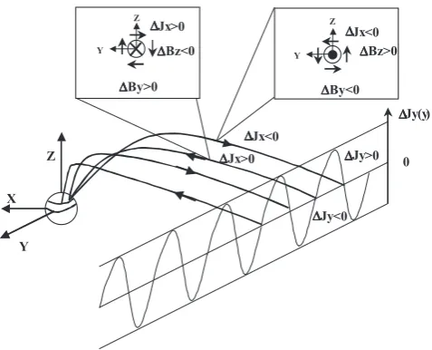
Fig. 5. Schematic view of the parallel current system corresponding

to an azimuthal modulation of the cross tail currentJy. The top panel inserts display the local magnetic field perturbation produced by a tailward (resp. earthward) parallel current (∼Jx).

(e.g. Asano et al., 2005; Runov et al., 2006), the thin one tends to be carried by the electrons, while the wider one is still carried by ions. In that case, the ion speed in the cen-ter would be reduced (and could even be reversed). A KH analysis by Lapenta and Knoll (2003) indeed shows that KH instability can be excited and propagate in the general cur-rent and ion flow direction, even when the ion flow velocity is reversed in the center.

These modes may provide an explanation for waves prop-agating across the tail, but they do not necessarily lead to a net reduction and diversion of the cross-tail current. There are two major plasma instabilities considered for such cur-rent disruption. The first one is the current-driven elec-tromagnetic ion cyclotron instability (Perraut et al., 2000). For this model, the formation of a thin current sheet dur-ing the growth phase is described as an externally applied time-dependent perturbation, localized in the azimuthal di-rection. The timescale of the perturbation is assumed to be larger than the ion and electron bounce periods. The kinetic response of the plasma, taking into account the bounce mo-tion of particles due to the mirror geometry of the near-Earth magnetotail, implies the development of an electrostatic po-tential constant along a given magnetic field line (Hurricane et al., 1995). The corresponding potential electric field tends to shield the induced electric field due to the stretching of the magnetic field lines. Therefore the perpendicular motion, at least in the near equatorial region, is partly inhibited (Le Contel et al., 2000a,b). This can explain why CS thinning (or oscillations of CS) are not necessarily accompanied by an az-imuthalEy, and hence by an earthward or tailward flow.

On the other hand, the increase of the cross-tail cur-rent in an azimuthally localized region, during the growth

phase implies an increase of the parallel current in or-der to ensure the zero divergence of the total current (∇·j∼∂jy/∂y+B∂/∂l(jk/B)∼0, wherelis the length along

a field line). The radial component of the current can be neglected assuming that the radial scale length of the perturbation is larger than the azimuthal and field-aligned scale lengths. For a large enough parallel current, “high-frequency” current- driven Alfv´en waves (CDA) in the range of proton cyclotron frequencies are driven unstable. As they propagate along field lines, CDA waves can undergo two types of resonances. In the CS the waves interact with elec-tron via bounce resonance. As they propagate away from the equatorial region, CDA waves are mode converted into shear Alfv´en (SA) waves and the phase velocity (essentially the Alfv´en speed) becomes of the order of the electron thermal velocity. In such conditions, CDA/SA waves are able to pro-duce electron parallel diffusion. For intense CDA/SA waves, the diffusion time (τd) of electrons via CDA/SA waves is

equivalent to the bounce time (τb), which has two important

consequences (Le Contel et al., 2001b,a): (1) The parallel current is disrupted, therefore the equilibrium is broken and the perpendicular current must also vanish, thereby produc-ing a local dipolarization, in agreement with observations; and (2) the non-local response associated with the electron bounce motion vanishes. The induced electric field corre-sponding to the local dipolarization, is no longer shielded and produces transient fast flows. Therefore, on the timescale of electron diffusion, large electric fields can exist and produce enhanced electric drift and the corresponding fast flows.

The previous scenario has been described in the context of the quasi-static evolution of a current sheet, for instance during the growth phase. It also applies to a situation where low-frequency modes, for instance ballooning modes, spa-tially modulate theJy current (Pellat et al., 2000). As

de-picted in Fig. 5, the spatial modulation ofJyimplies a series

of field aligned currents that eventually turn out to be un-stable, when the parallel current increases, that is when the parallel drift between electrons and ions gets large enough. The magnetic signatures of these parallel currents are also depicted in Fig. 5. At Cluster orbit, parallel currents will essentially be radial, hence the corresponding magnetic sig-natures,δB, will be in theY Zplane. Thus, in this model, the fluctuations observed inBy andBzare interpreted as

signa-tures of parallel currents associated with azimuthally propa-gating structures carrying parallel currents (as illustrated in the figure). Thus the interpretation of the quadrupolar sig-nature onBy, and bi- polar signature onBz, as the signature

of Hall currents associated with an X-line (see Fig. 4) mov-ing vertically (reversal ofBy) or radially (reversal ofBz), is

soon as the absolute value of magnetic perturbation, associ-ated with the perpendicular current perturbation, exceeds the weak dipole field. Off equator, where parallel current pertur-bations are stronger, correlatedByandBzperturbations can

be associated with an azimuthal motion of the mode. The second candidate for current driven instability is the cross-field current instability (Lui, 1991). For this paradigm, enhanced current density in the tail current sheet due to ki-netic ballooning instability (Cheng and Lui, 1998) or to any process responsible for the explosive growth phase (Ohtani et al., 1992) is assumed to occur just prior to current disrup-tion. This leads to the excitation of the cross-field current instability with high frequency perturbations from oblique whistler waves. The resultant development of this instabil-ity leads to turbulent environment with waves over a broad frequency range from about the ion cyclotron frequency to lower hybrid frequency. These oblique whistler waves can give rise to quadruple By perturbations outside the current

disruption region. This activity associated with this kinetic instability is spatially localized initially.

Most researchers associate moderate- and high-speed plasma flows with magnetic reconnection. However, cur-rent disruption can lead to force imbalance and consequent plasma acceleration to high-speed plasma flows as well (Lui et al., 1993). Figure 6 illustrates schematically the expected loss of equilibrium from current disruption (Lui, 2001). The top part of the figure shows that before occurrence of cur-rent disruption, the curcur-rent density in the curcur-rent sheet varies rather smoothly across the sheet. During current disruption, the current density becomes highly inhomogeneous, ranging from reversed current flow to enhanced current density with the overall current reduction averaged over the entire region. The nonlinear evolution of the plasma instability or instabili-ties responsible for current disruption leads to large magnetic fluctuations, especially in theBzcomponent, as depicted in

the middle of Fig. 6. In the near-Earth region, the ambient magnetic field componentBz is strong. The netBz is thus

mostly northward because the Bz fluctuation seldom goes

southward large enough to overcome the ambient field. In this region, the amount of current reduction due to disruption typically is smaller than the increase of magnetic field due to current reduction. This is because the current enhance-ment prior to current disruption suppresses the dipolar field contribution to the local magnetic field. Current reduction results in diminishing this suppression and thus an increase of magnetic field. There is thus a net increase in the j×B force in this situation. On the other hand, in the mid tail re-gion the ambient magnetic field is weak. The net magnetic field therefore becomes frequently negative. When the net

Bzis negative, both j×B and pressure gradient forces

accel-erate the plasma tailward. Even when the netBz is positive,

the current reduction can become larger than the associated magnetic field increase. This leads to a net decrease in the j×B force and, again, a consequent tailward plasma acceler-ation. The above consideration indicates that there would be

Cross-Tail Current Before Current Disruption

Cross-Tail Current During Current Disruption

CD

Bz Bz

Earthward Flow Tailward Flow

J B J _× B

δ_Bzfrom CD

J B J × B

Time Time

Fig. 6. Schematic of how small-scale fluctuations from localized

current disruptions might lead to organized earthward or tailward flow. After Lui (2001).

some association between tailward plasma flow and south-wardBz but deviations from this association is expected to

occur occasionally, e.g., tailward flow with northwardBzor

earthward flow with southwardBz.

3 Description of events

Thin current sheets with a thickness comparable or less than the Cluster tetrahedron scale are observed under different conditions. Here we describe current sheet crossings from two Cluster 2001 tail periods, when the tetrahedron scale was about 2000 km and the spacecraft were near apogee in the premidnight sector (Fig. 7). The first event, between 20:40 and 22:00 UT on 7 September 2001, consists of two different types of current sheet: (a) a thin current sheet during a quiet interval and (b) a current sheet during a pseudo-breakup. The second event shows (c) a current sheet with a flow reversal and hence a possible X-line signature during a storm-time substorm, between 09:20 and 09:55 UT, on 1 October 2001. In the following we briefly describe the global context of the events in Sect. 3.1 and highlight the specific observed fea-tures for these events in Sects. 3.2–3.3. Finally, the key ob-servations are summarized in Sect. 3.5.

3.1 Overview of the selected events 3.1.1 7 September 2001

0 -10 -20 XGSM 10 0 -10 YGSM

0 -10 -20 XGSM -10

0 10

ZGSM

10 0 -10 YGSM -10 0 10 ZGSM Oct 1

Oct 1 Oct 1 Sep 7

Sep 7 Sep 7

2001-10-01 09:20UT

1000 -1000 -3000 ΔXGSM 3000 1000 -1000

Δ

YGSM

1000 -1000 -3000 ΔXGSM -1000

1000 3000

Δ

ZGSM

3000 1000 -1000 ΔYGSM -1000 1000 3000 Δ ZGSM 2001-09-07 20:40UT

2000 0 -2000 ΔXGSM 2000

0 -2000

Δ

YGSM

2000 0 -2000 ΔXGSM -1000

1000 3000

Δ

ZGSM

2000 0 -2000 ΔYGSM -1000 1000 3000 Δ ZGSM b a c e d f h g i

Fig. 7. Cluster location for the 7 September and 1 October events

and tetrahedron configuration for 7 September and 1 October event.

happened at the end of the selected time interval, around 22:00 UT. The Image and Polar spacecraft (data not shown) give evidence for an auroral bulge developing near the Clus-ter footprint, at about 21:29 UT. This bulge has a small ex-tension in latitude, around 70◦MLat. Hence Event 1 is not a fully developed substorm; it corresponds to a localized (in latitude) perturbation propagating eastward at ∼50 km/s in the ionosphere, presumably a pseudo-breakup.

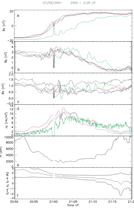
Figure 8 shows spin averaged field and particle data. Three components of the magnetic field in GSM coordinates ob-tained by the FGM magnetometer (Balogh et al., 2001) are shown in Figs. 8a–c. The DS2 component of the electric field data from EFW (Gustafsson et al., 2001) is shown in Fig. 8d (the DS2 component is approximately parallel to−Y in GSE coordinates). Here we changed the sign of the DS2 component so that it is close to the dawn-to-dusk electric field, Ey. X and Y components of the proton bulk flow

from the CIS/CODIF experiment (R`eme et al., 2001) are shown in Figs. 8e and f.XandY components of the current density calculated from the linear curl estimator technique (Chanteur, 1998), using FGM data are shown in Fig. 8g. It should be kept in mind that Cluster estimates the averaged current density on the scale of the tetrahedron, i.e., 2000 km. Finally, panels (h) and (i) show the parameter for protons and oxygen, respectively. Values ofβup to 100 are measured for protons andβ>1, for oxygen. Yet, in spite of this high-β, thin CS remains stable and quiet.

2001-09-07 (jx:black, jy:red)

-20 0 20

BX [nT]

-20 0 20

BY [nT]

-20 0 20

BZ [nT]

-5 0 5

EDS2 [mV/m]

-400 0 400 800

VX [km/s]

-400 0 400 800

VY [km/s]

-20 0 20

j X,Y [nA/m/m]

0.01 0.10 1.00 10.00 100.00 beta(H+)

20:40 20:50 21:00 21:10 21:20 21:30 21:40 21:50 22:00 0.01 0.10 1.00 10.00 100.00 beta(O+) a d c b e h g f i

Fig. 8. (a, b, c): spin resolution data from GSM components of

the magnetic field, (d) DS2 component of the electric field, (e, f) GSM X,Y components of the proton bulk velocity, (g) current den-sity determined from the magnetic field, (h, i) proton and oxygen beta. For the particle and field plots, profiles for Cluster 1, 2, 3, 4 are plotted with black, red, green, and blue lines, respectively. Black and red lines in the current density plots correspond to X and Y components.

Quiet CS crossing

Between 20:40 and 21:30 UT, theBxcomponents vary from

approximately−12 nT (at S/C 3) to +18 nT (on S/C 4; see Fig. 8a), hence the four S/C cross the magnetic equator. Dur-ing this crossDur-ing the CS is relatively quiet; the dawn-dusk electric field (Fig. 8d) and the ion flows in the X direction (Fig. 8e) are weak and the magnetic fluctuations are small (panels a, b, and c). The most rapid variation is along the Z direction. Then the CS thickness can be estimated from the difference between the values ofBx, measured at the four

S/C locations; this is done in Sect. 3.2.2. Around 21:00 UT S/C 3, which is at a lowerZthan its 3 companions, is located at the CS boundary, while S/C 1, 2 and 4 are located close to the magnetic equator. Hence the half-thickness of the current sheet should be of the order of the distance, projected along

at about 21:00 UT. Knowing the CS thickness, one can es-timate the current density,Jy≈1Bx/µ0H≈10 nA/m2, con-sistent with the value calculated from curl B (panel g). For this event, however, the characteristic spatial scale of the cur-rent sheet is comparable to the distance between the satel-lites. Therefore, the current density obtained from the cur-lometer method can only be considered as a rough estimate (in fact an underestimate). During this quiet CS crossing the ion flow velocity is sufficient to account for the estimatedJy.

Indeed forN≈1/cm3, andVy≈50 km/s (estimated from CIS)

we findJy≈8 nA/m2. Hence during this quiet CS crossing

the current, in the S/C frame, is essentially carried by ions.

Active CS crossings

From 21:30 to 21:42 UT, the averaged value ofBx, for S/C 3,

varies from positive to negative. Large amplitude oscilla-tions inBy and Bz are superimposed. Hence, the current

sheet structure is three-dimensional. On the other hand, the fluctuations inBx , detected by S/C 1, 2 and 4, are weaker,

andBxremains close to the lobe value (∼20 nT). Therefore

S/C 1, 2 and 4 are located outside the CS, or close to CS boundary layer, at least till 21:46 UT. Thus, between 21:30 and 21:46 UT, the CS thickness must be smaller than the dis-tance between SC 3 and its companions projected alongZ

(∼1500 km). After 21:45 UTBxat S/C 1, 2, 4 decrease, on

average, and oscillate, whileBxat S/C 3 becomes negative.

Hence the CS thickness becomes comparable to the distance between the S/C. Using the value ofBx, normalized by the

lobe value (∼20 nT), as a proxy to estimate how far a given S/C is located away from the center of the CS, we find that large ion flow velocities (Vx) are found close to the equator.

The reverse is not true: being at the equator does not warrant the observation of a fast ion flow. Notice that large amplitude variations inEy(Fig. 8d) are also observed.

Surprisingly the ion velocity in the Y direction, which was positive (as expected) before 21:30 UT, becomes neg-ative (eastward) around 21:35 UT, and sometimes reaches

−200 km/s. The westward current must be carried by elec-trons moving eastward, faster than ions; this is further dis-cussed in Sect. 3.2.2. Asano et al. (2004) have also given evidence for westward currents carried by electrons, in the case of a Geotail event.

Thick CS

After 21:52 UT, all s/c measure almost the sameBx∼0

in-dicating that the spatial scale of the CS is now much larger than the distance between the satellites. During this period, the current densityJy (panel g) is smaller than before. Note

that after 21:55 UT, a short lasting thinning of the CS occurs again, while enhancedVxis detected.

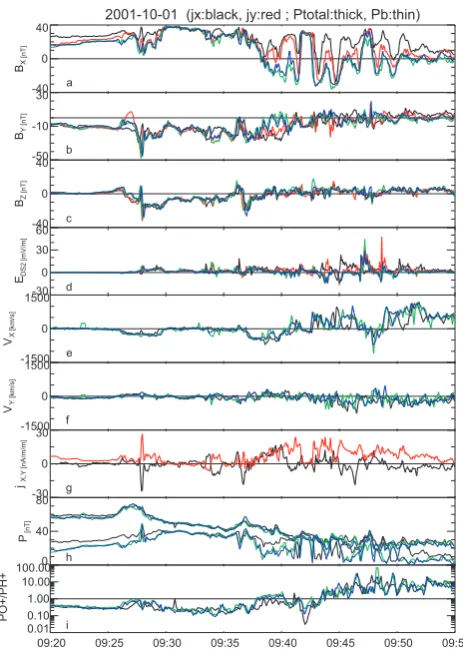
2001-10-01 (jx:black, jy:red ; Ptotal:thick, Pb:thin)

-40 0 40

BX [nT]

-50 -10 30

BY [nT]

-40 0 40

BZ [nT]

-30 0 30 60

EDS2 [mV/m]

-1500 0 1500

VX [km/s]

-1500 0 1500

VY [km/s]

-30 0 30

j X,Y [nA/m/m]

0 40 80

P [nT]

09:20 09:25 09:30 09:35 09:40 09:45 09:50 09:55 0.01

0.10 1.00 10.00 100.00

PO+/PH+

a

d c b

e

h g f

i

Fig. 9. Same format as Fig. 8 except for the bottom two panels,

which are: (h) total and magnetic pressure, and (i) ratio between oxygen and hydrogen pressure. In the pressure plot the total and the magnetic pressures are plotted with thick and thin lines, respec-tively.

3.1.2 1 October event

Between 06:00 and 16:00 UT on 1 October, a series of semi-periodic substorms took place. The interval has a charac-teristic of a “saw-tooth” event during a large storm with a minimum SYM-H of 150 nT at 08:30 UT. The interplane-tary magnetic field (IMF) was directed southward during the whole interval and ranged betweenBz=−15 and−2 nT. In

this study we examine Cluster observations during the sec-ond substorm interval, when a LANL geosynchronous satel-lite (1991-080) detected multiple dispersionless electron and ion injections starting at 09:26 UT and a large substorm with AE>1000 nT took place. As shown in Figs. 7a–c, Cluster was located atXGSM=−16.4RE, nearZGSM=0 in the

pre-midnight magnetotail. The Cluster tetrahedron configuration at 09:20 UT is shown in Figs. 7g–i.

Here the particle pressure was calculated using both proton and oxygen. We converted the pressure value into an equiva-lent magnetic field value (in nT), so that the likely lobe field strength can be inferred from the total pressure. The ratio between oxygen and hydrogen pressure is shown in Fig. 9i.

As can be seen from Bx (Fig. 9a) and from the relative

Cluster positions (Figs. 7e and f), the ordering of decreas-ingBx values, i.e., Cluster 1, then 2, then 4, and finally 3,

is consistent with the relative order of the Cluster positions from north to south most of the time, suggesting that the tail current sheet orientation is approximately perpendicular to

ZGSMand thatBxgives a good indicator of the location

rel-ative to the equator, on long time average. Yet, there are intervals with short-time perturbations or rapid current sheet crossings lasting less than a minute where the current sheet were significantly tilted from nominal orientation as will be discussed in more detail in Sect. 3.3. Cluster was initially located close to the northern lobe. Because of the high solar wind pressure and larger flux in the tail during a storm, the lobe field value during the initial interval is expected to be larger than 40 nT, as can be seen in theBxcomponent when

Cluster enters the lobe between 09:30 and 09:33 UT. After 09:37 UT, Cluster experienced several neutral sheet cross-ings until 09:53 UT, when all the spacecraft stayed in the plasma sheet. The first signatures of substorm disturbance at Cluster are the magnetic field fluctuations accompanied by tailward proton flow and encounter of the plasma sheet start-ing at 09:26 UT, which corresponds to the time of geosyn-chronous injection. After the plasma sheet encounter the to-tal pressure started to decrease with some fluctuations and became 30 nT by 09:50 UT and stayed nearly the same value afterwards. This negative trend in the pressure is a typical manifestation of unloading in the mid tail region during sub-storm expansion phase. As is often the case for a sub-storm, the oxygen contribution is significant, as shown in Fig. 9i. Par-ticularly after 09:44 UT the pressure is dominated by oxygen. This corresponds to the time interval of the thin current sheet as will be described later.

There were mainly two periods of enhanced tail-ward/earthward proton flows during the interval (Fig. 9e). The first one is the tailward flow between 09:26 and 09:30 UT near the geosynchronous injection time. Associ-ated with this first tailward flow period (at about 09:27 UT), a sharp enhancement inByand a positive, then negative

dis-turbance inBzof about 30 s is observed, which is the typical

signature of a tailward moving flux rope. The disturbance is accompanied by a large spike in the current density. This current is directly parallel to the ambient field flowing out from the ionosphere. Such<30 s structures withBz

rever-sals andByperturbations are identified also during the next

flow enhancement intervals.

The second flow interval is from 09:37 UT, and contin-ues until 10:04 UT (not shown), with several flow reversals from tailward to Earthward and vice versa on a timescale of>10 min containing also rapid fluctuations. TheBz

pro-file in Fig. 9c also shows corresponding sign reversals on longer and shorter time scales: i.e., negative values on aver-age, during predominantly tailward flow period and positive value mainly during Earthward flow periods, overlapped with faster fluctuations. The overall relationship betweenBz and

flow, on greater than 10-min scale, is in a sense of producing dawn-to-duskV×B electric field. Consistently, the dawn-to-dusk electric field from EFW (Fig. 9d) became enhanced during the flow intervals exceeding several mV/m (up to 10 mV/m). Between 09:43 and 09:58 UT, even stronger elec-tric fields were observed associated with neutral sheet cross-ings. Detailed field and plasma signatures between 09:46 and 09:51 UT, when strong electric fields, flow reversals and neutral sheet crossings were observed, will be discussed in Sect. 3.2.1.

Starting around 09:37 UT, when Cluster encountered the plasma sheet and observed tailward flow, persistent oscilla-tions also started in theBxprofile (Fig. 9a) with a time scale

of about 2 min. Based on minimum variance analysis of each crossing and timing analysis of the four spacecraft, these os-cillations are due to a wavy current sheet. Assuming that the propagation vector identified from the current sheet cross-ings represents the motion of the current sheet, it is expected that the motion of the wavy current sheet is mainly duskward with a speed of 100–300 km/s. From this speed and the 2 min recurrence it is estimated that these wavy structure has a cross-tail spatial scale of 2–6RE. It should be also noted

that the inter-spacecraft difference inBx stands out during

this period (Fig. 9a). The profile shows that the half thick-ness of the current sheet is expected to be smaller than the Cluster tetrahedron. The duskward current density obtained from the Cluster increases up to 20 nA/m2.

Another important observation for this event is the ion composition. During the thin current sheet interval, 09:45– 09:55 UT, pressure as well as density was dominated by O+ (Kistler et al., 2005), which was interpreted as being due to storm-time ion outflow. In this O+ dominated thin current sheet, the O+ions were observed to execute Speitype ser-pentine orbits across the tail and were found to carry about 5–10% of the cross-tail current (Kistler et al., 2005). De-tailed analysis of the distribution function showed separate O+ layers above and below the thin current sheet (Wilber et al., 2004).

3.2 Crossing of a quiet CS; 7 September 2001, 21:00 UT Figure 10 (panels a, b, and c), shows thatBxchanges from

about−20 nT to +20 nT, whileByandBz(plotted here with

a different scale) and their fluctuations, are small (few nT). The current densitiesJy, estimated by various methods are

shown in panel (d). Since the current sheet is essentially per-pendicular toZGSM, we have fitted theBxcomponent of the

of the current sheet, respectively. BL can be obtained

ei-ther from direct measurement in the lobe region (if the S/C happens to be located in the lobes) or by assuming the equilibrium of the vertical pressure within the plasma sheet (Baumjohann et al., 1990; Kivelson et al., 2005; Thompson et al., 1993). Here, for both periods,BL≈25 nT. Once these

parameters are determined, we compute and plot the Harris current density at the equator (thick pink line), and at the lo-cation of S/C 3 (thick green line). We also plot the current density estimated from curlB(thin pink line) and the contri-bution of the ions computed from CIS measurement on S/C 3 (thin green line).

Assuming that the current density profile is stationary dur-ing the crossdur-ing of the CS we find thatJyis maximum near

the center of the CS and thatJy_max≈10 nA/m2. The ion

cur-rent is also quite close to the other estimates, which suggests that during the quiet crossing most of the current is carried by ions, in the s/c frame. The contribution of electrons to the current (not shown here) is indeed small. Jx(not shown

here) is much smaller thanJy(panel d).

The fit with a Harris sheet has also been used to estimate the half-thickness of the CS (H). In order to getHwe choose a couple of s/c with similar values of Y and (if possible

X), but different values ofZ. This choice aims at minimiz-ing the possible effects of radial and azimuthal modulations upon the determination ofH. Figure 10e shows that, around 21:00 UT,H≈2000 km. During this period all the S/C are located inside the CS, hence the fit is good. The increases inH found around 20:50 and 21:20 UT are probably not reliable, because the S/C get too close to the CS boundary. Figure 10f shows the position of the CS center (Z0), and the estimated location of its lower (Z0−H) and upper (Z0+H) boundaries, deduced from the same fitting procedure. It tells us that the CS moves southward at about 5.5 km/s, in the S/C frame. Cluster spacecraft move slowly southward (∼2 km/s); thus the CS moves at about 7.5 km/s. The motion of the CS can also be inferred from the time (∼10 min) it takes to cross the CS (2×2000 km). With these numbers we find that the CS center moves southward at about 7 km/s; consistent with previous estimate. Noticing that S/C 1, S/C 2, and S/C 4 are approximately at the sameZGSM, the delay between the crossing of the center of the CS can be used to characterize the flapping of the CS.

In summary a relatively thin CS (half thickness of about 2000 km) can be stable over long time periods. For

N∼cm−3_,V

t hi∼1000 km/s, andFH+≈0.15 Hz (lobe field),

we get the H+ _{ion Larmor radius and ion inertial length} ρi∼L∼1000 km, i.e., half the CS half-thickness. As already

mentioned, while describing Fig. 8, magnetic fluctuations are weak and no fast flow is observed during the crossing of this quiet but relatively thin CS. The slow flapping oscillation does not affect the stability of the CS.

a

b

c d

e

f

Fig. 10. Quiet CS crossing. Notice thatBy andBzare not at the same scale asBx; most of the magnetic field variations are onBx, as expected for a 1-D CS. Panel (d) shows (i) Harris current density at the equator (thick pink line), (ii) at the location of S/C 3 (thick green line), (iii).Jyfrom curlB (thin pink line) and (iv) contribution of ions toJy, computed from CIS measurement on S/C 3 (thin green line); panels (e) and (f) show the half- thickness (H) of the CS and the location of its center (Z0). Time resolution is 4 s.

3.3 Crossings of an active CS, 7 September 2001, 21:30– 21:55 UT

3.3.1 Magnetic fields and current densities

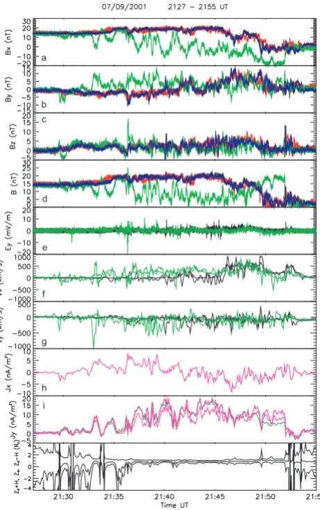
The four top panels of Fig. 11 show again theBx,By, Bz,

the modulus ofB, and the−SR2 component of the electric field (essentiallyEy), with an enlarged scale. Magnetic and

electric field data are now displayed with full resolution (22.4 points/s for B and 25 points/s forEy). The averaged motion

of the CS, as inferred from the averaged variations ofBx, is

now upward. Panel (i) showsJy, estimated from curlB.

a

b c

d

e

f

g

h i

j

Fig. 11. Crossing of an active CS (September 7, 2001). From top

to bottom, high time resolution data from FGM (Bx, By, Bz,B) and EFW (Ey). Unless otherwise noted, black is for S/C 1, red for S/C 2, green for S/C 3 and blue for S/C 4.Vx ifrom CIS (thick line) andV_{x e}from PEACE (thin line) on S/C 1 and S/C 3, same forVy,.

JxandJy(thin pink line), computed from curlB, equatorial current density (thick pink line) and at the location of S/C 3 (thick green line) from Harris model (thin pink line), withBL=25 nT (see text for more details).

the Harris fit and the current density computed from curl B agree quite well. Between 21:33 and 21:45 UT S/C 3, which is the only s/c located inside the CS, detects large amplitude, about 1 min quasiperiod fluctuations. The large amplitude fluctuations observed onBx(3) can be due (i) to a

modula-tion of the total currentIybelow the S/C, (ii) to a flapping of

the CS (with a large amplitude∼D), or (iii) to a modulation in the CS thickness (H). Bx at S/C 1, 2, 4 (outside the CS)

being almost constant, interpretation (i) is ruled out. Thus the CS thickness is modulated (symmetric mode), or the CS flaps up and down (anti-symmetric mode), or a mixture of both. Whatever the mode, the fact thatBx(3) can be

nega-tive, whileBx(1,2,4) remain approximately constant and

pos-itive, indicates thatHis comparable to, or even smaller than

D. The fluctuations ofZ0+H are much larger than that of

Z0−HandZ0(see the last panel of Fig. 11), which suggests that the oscillations are asymmetric, or that S/C 1, 2, 3 are outside the CS, and therefore do not probe the fluctuations which are highly confined in the CS. In fact the LF modes can provide a proxy for the accuracy of the estimate ofZ0 andH. In the later caseZ0andHare not correctly estimated. For instance, around 21:35 UT,H is probably largely over-estimated and the largely negative value ofZ0should not be trusted. Yet we can infer that between 21:33 and 21:45 UT,

H <D≈1500 km, and that the total current inside the CS is essentially constant. Conversely after 21:45 UT, the three other S/C (S/C 1, 2, 4) penetrate in the CS; the estimates via the Harris fit are now accurate. A symmetric sausage like behavior is observed, with a constantZ0and symmet-ric variations of Z0+H and Z0−H. Between 21:45 and 21:52 UT, whereH≈1500–2000 km, large earthward flow bursts are observed (up to 600 km/s). After 21:52 UT, H

rapidly increases;HD. At the scale of the tetrahedron, the magnetic energy has been dissipated since B is quasi-null on all spacecraft. There are no longer large flow velocities. Thus the large amplitude quasi-periodic (60 s) fluctuations are strongly confined in the CS and they develop only when the CS is thin, or very thin (21:33–21:45 UT). The thickening of the CS, and therefore the local dissipation of the magnetic energy, starts around 21:45 UT. After 21:52 UT, the CS gets very thick (∼2RE); the magnetic energy has been dissipated

and the transport of particles stops by 21:54 UT.

When the CS is thin or very thin, the fluctuations ofByand

Bzare quite large, in particular (but not only) on S/C 3. These

fluctuations are interpreted as signatures of field aligned cur-rents (see Sect. 4). Panels (h) and (i) showJx andJy,

esti-mated from curlB. Firstly, we observe a signature of nega-tive parallel current (Jx<0) between 21:29–21:30 UT

asso-ciated withVx<0 (tailward) andVy<0 (dawnward), for

elec-trons as well as for ions (see also Le Contel et al., 2002, and references therein), which suggests that the active region is localized earthward or westward of the S/C (see discussion in Sect. 4). In this current density structure the current is essentially antiparallel toB, and the spatial scale is compa-rable or smaller thanD, as can be seen from theByandBz

profiles on S/C 3. Hence, the current density from the cur-lometer (Jx≈−5 nA/m2) is probably underestimated. More

generally, bothJyandJxare likely to be underestimated, at

least during the first period (21:33–21:45 UT). The fluctua-tions ofJx(panel g) are as large as the fluctuations ofJy(as

expected from∇·J=0). Thus, unlike the previous crossing (at about 21:00 UT) the structure of the active CS is now 3-D. The signatures of the FAC are seen onBy, as expected, but

also onBz, which indicates that they have a small scale in the

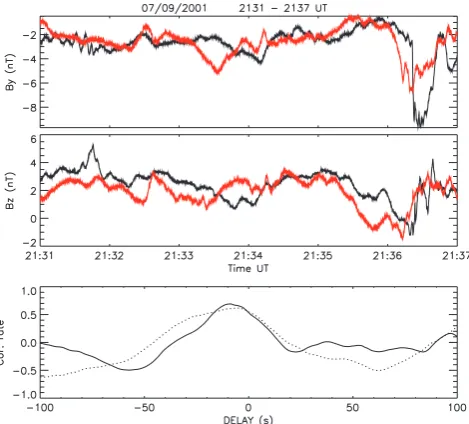
Fig. 12. By andBz on S/C 1 and 2 at high-time resolution on 7 September between 21:31 and 21:37 UT. The full line is for the correlation function betweenBy(1) andBy(2), the dotted line gives the correlation function betweenBz(1) andBz(2). Time resolution of the correlation is 0.4 s.

(about a few nT,∼1–20 mV/m), but still smaller than long period oscillations, at least for the magnetic components. We do not further discuss about these “high frequency” oscilla-tions here.

In order to determine the direction of propagation of the CS fluctuations we correlate high time resolution data at S/C 1 and 2. The corresponding wave forms and correla-tion coefficients are displayed in Fig. 12. S/C 1 and 2 are essentially separated alongYGSM, by∼2000 km, while they are located at about the sameXGSM and ZGSM. Thus the delay obtained from the correlation lag (∼10 s) corresponds to an eastward motion at∼200 km/s, in the same direction as electrons that carry the current in the S/C frame. In or-der to identify the 3-D characteristics of the fluctuations, we compare the four spacecraft magnetic field wave forms dis-played in Fig. 13a (top panels). During this short time in-terval (40 s),By(3) undergoes a positive excursion (+10 nT

at 21:36:10 UT), whileBy(1),By(2), andBy(4) get negative.

The extrema ofBy, at the locations of the various S/C, are not

simultaneous, as depicted by the vertical dashed lines. The delays between the extrema ofBy, at the various S/C, can be

due to a radial or to an azimuthal motion. For S/C 1, 2 and 4 the dashed lines roughly correspond to zeros ofBz, but the

maximum ofBy(3), at 21:36:20 UT, does not coincide with

a zero ofBz(3). Instead it coincides with the maximum of

Bx(3). These observations are discussed in Sect. 4.2.1 where

they are used to infer the shape and the motion of the corre-sponding structure.

Fig. 13. (a) Magnetic field data between 21:36:00 and 21:36:40 UT,

7 September 2001. (b) Hodograms of the magnetic field projected onto the (XY) plane during the time interval shown in panel (a). Spacecraft are ordered by their locations alongZ. Bx is a proxy for the location of each S/C with respect to CS centre. Vertical dashed lines indicate the estimated closest approach, for each S/C. Dashed circles are drawn only for S/C4 (for clarity); they are tan-gent to magnetic field direction (inBy,Bzplane) taken at 3 selected times. To single out the magnetic field vectors corresponding with the selected times, we have extended their lengths via dashed ar-rows. Then the magnetic field direction is used for a remote sensing of the motion of the center of current tube. As discussed in the text the current tube is found to move eastward.

Figure 13b (4 lowest panels) shows hodograms ofBy,Bz

for the four S/C.Bx is used as a proxy for the position of

each S/C with respect to CS center. Then the hodograms represent the projections ofB on the (By, Bz) plane, as a

function of time, at the location of the S/C, inferred fromBx.

a

b

c

d

e

f

g

h

i

j

Fig. 14. (Flow reversal. Same format as Fig. 11. For this event

BL=40 nT. The parameters of the Harris sheet are determined from

Bxmeasured by S/C 1 and 3, at differentZand similarXandY. Panel (i) shows the two independent time profiles ofJ, estimated from Harris fit (thick pink,) and from curlB (thin pink). The green line is forJat S/C3, from Harris fit. CS parameters (H andZ0) are

determined from S/C 3 and 4. Data displayed in panels (f, g, i, j) are deduced from CIS/CODIF. Here time resolution of CIS data is 8 s.

evidence for rotations of the magnetic field, with compara-ble amplitudes alongY andZ, at least on S/C 3. In order to visualize the relation betweenδBand a possible motion (ra-dial/azimuthal) of the structure, we have selected three par-ticular instances and used the corresponding magnetic field vectors (dashed arrows in 13b) to track the position of the center of the structure and to follow its motion. The results are discussed in Sect. 4.2.1.

3.3.2 Ion and electron velocities

Figure 11 shows the ion and electron velocities, computed from CIS and PEACE, for S/C 1 and S/C 3. The short lasting

parallel current structure, around 21:29–21:30 UT, is associ-ated with tailward ion and electron velocities, which can cor-respond to an active region developing earthward of the S/C. This is followed by bursty earthward ion and electron flow velocities (V_{x i,e}) starting to develop first at S/C 3 (at about 21:33 UT), together with the fluctuations, as the spacecraft penetrates deep in the CS. The velocities are now earthward, suggesting that the active region is now tailward of Cluster. Large velocities are observed later at the other S/C, once they have penetrated in the CS (after 21:46 UT). Finally, between 21:50 and 21:52 UT,Bx≈−20 nT at S/C 3; whileBxclose to

zero at S/C 1, 2, 4, thus S/C 1, 2, 4 are now close to CS cen-ter while S/C 3 is near its southern boundary. ThenVx ihas

moderate values at S/C 1, 4 and is small at S/C 3. Thus, in this thin and active CS, the ion velocity maximizes near the CS center and vanishes at its boundary. The average values ofVx efollowVx i, but short lasting bursts ofVx eoccur, with

no ion counterparts.

In order to produce the westward current supporting the CS a substantial westward ion velocity (∼100–200 km/s) is expected. As already shown by Fig. 8, V_{y i} is small and negative; ions cannot carry the westward current. Fig-ure 11g shows that V_{y e} is negative and larger in absolute value thanV_{y i}; in averageV_{y i}−V_{y e}≈100–200 km/s, hence forN∼1/cm3we getJy≈15–30 nA/m2; somewhat above the

estimate from curlB. Given that curlBunderestimatesJy, a

current densityJy≈15–30 nA/m2seems realistic. This value

corresponds toH≈500–1000 km which is comparable to, or smaller than, ρi, the ion Larmor radius (∼1000 km) in the

lobe field. In Fig. 11 we see that the estimate ofJyvia curl

B is between the estimates (via a fit with an Harris sheet) of the current density at the equator and at S/C 3, thereby confirming the validity of these estimates; at least as long as

D≈H.

3.4 Active CS with flow reversals, 1 October 2001, 09:46– 09:51 UT

3.4.1 Current sheet structures during rapid current sheet crossings

Figure 14 shows the magnetic field, electric field, and ion data in the same format as Fig. 11, but during the second event, between 09:46 and 09:51 UT. Consecutive north-south excursions of the current sheet are observed during this in-terval with a time scale of about 1–2 min. By estimating the velocity of the current sheet motion using the tempo-ral changes ofBxand spatial gradient ofBx, profiles of the

current sheet thickness was found to be less than the tetrahe-dron scale (Runov et al., 2003; Wygant et al., 2005), while it is broad (∼4000 km) or bifurcated during the 09:48:00, 09:49:30, and 09:50:00 UT crossings (Runov et al., 2003). While the parameter of the Harris-type current sheet gives generally a good indicator of the scale of the current sheet, these internal structures deviating from a Harris-type current sheet profile and the relatively large separation of the Cluster S/C compared to these thin current sheet period could explain why the current sheet was estimated to be continuously thick at the bottom of Fig. 11 during this particular event.

TheByprofile involves changes with time scale of the

or-der of the duration of the current sheet crossing (as discussed above) and more transient peaks. During the first two cross-ings, when the flow is tailward, the general trend ofBy is

anticorrelated with that ofBx. On the other hand, after the

09:48:30 UT crossing,By andBx profile during the

cross-ing is correlated. In addition to this trend, there are transient peaks on a 10-s time scale, such as the one clearly seen on C2 and C4, around 09:48 UT. The same is true forBz;

tran-sient variations are superimposed on a (longer time scale) negativeBz during tailward flow and a positiveBz during

Earthward flow. TransientBzpeaks or reversals are observed

around 09:47:10, 09:47:45, 09:48:50 UT. The strongest tran-sient peaks, onBy andBz, are found around 09:47:45 UT;

they will be later discussed in more detail.

Reversals of the electric field are associated with the cross-ings around 09:47:00 UT and 09:48:30 UT, during the thin current sheet crossings. The strongest electric fields were detected at the Northern Hemisphere, after the 09:46:50 UT crossing. Large amplitude fluctuations are also observed at much higher frequencies. “High frequency” electric fluctu-ations (up to 100 mV/m) are shown in Fig. 14. Magnetic fluctuations, δB2≈1–3 nT2, are also observed (not shown here) by STAFF. Furthermore, electrostatic waves with am-plitudes∼400 mV/m and frequencies varying from ion cy-clotron to lower hybrid, and electrostatic solitary waves with amplitudes of 25 mV/m and much higher frequencies were observed by the Electric Field and Wave (EFW) instrument during 09:47–09:51 UT (Cattell et al., 2005).

Energetic electrons (a few keV) are observed when the spacecraft is inside the CS, as monitored by the modulus of

Bx(see Fig. 15). Outside the CS proper, in the CS Boundary

Layer (CSBL), large fluxes are still observed, but at much lower energies; less than 1 keV. Notice also that the electron flux is very anisotropic; in the CSBL the electron flux (be-low 1 keV) is much larger in the parallel (bottom) and anti-parallel (top) directions than in the perpendicular (middle). Hence CSBL electrons show bi-directional electron fluxes. Disregard the lowest energy channel which is contaminated by photoelectrons. Interesting to note that the most ener-getic electrons are detected during the transientBz events

described before.

Fig. 15. Bx,By,Bzprofile (from FGM) and spectrogram show-ing the electron flux (from PEACE), color coded, versus energy and time, for S/C3 during the same time interval as Fig. 14. Time reso-lution is 4 s.

3.4.2 TransientBzreversals

Short duration By and Bz enhancements with reversals on

Bzare observed between 09:46–09:51 UT. The most

promi-nent structure occurs at 09:47:45 UT. Figure 16a is a blow-up showing this structure at an enlarged scale. S/C 1, the northernmost S/C hardly detects the signature of the struc-ture. This lack of detection suggests that the structure has a small size alongZ, and is located well below S/C 1. This is confirmed by the differences between the signatures at differ-ent S/C; the size of these structures should be smaller than the distance between the S/C (∼1500–2000 km), at least along

Z. The signature of the structure involves a large positive ex-cursion ofBy, at S/C 2 and S/C 4, with very similar temporal

profiles. The delay between theBy signatures at S/C 2 and

S/C 4 suggests a propagation of the structure, as discussed in Sect. 4.3.2. The maximum ofBy(2), red dashed line, is

associated with a reversal inBz(2). There is also a reversal

inBz(4), but there is a small time shift between the zero of

Bz(4) and the maximum ofBx(4). UnlikeBy(2) andBy(4),

By(3) does not yield a large excursion. YetBz(3) shows a

clear reversal, from positive to negative, with an amplitude as large as for S/C 4 and larger than for S/C 2. A large pos-itive excursion ofBx(3) is observed at the same time as the

reversal inBz(3). It is interesting to note that although

po-sition inZ and plasma data suggests C3 should be closer to the equator,Bx is larger at C3 than at C2 and C4 indicating

Fig. 16. 1 October 2001, event, same format as Fig. 13. Notice that

By(4) can be deduced fromBy(2) via a time shift of∼5 s (a). On

(b) dashed red circles are tangent to the magnetic field measured by

C2, at 3 successive times. Dashed lines are intended to single out the directions of theBfor these instances.

further illustrates the nature of the magnetic field structure at 09:47:45. The same presentation as for Fig. 13b is used. Spacecraft are again ordered by their positions alongZGSM. UsingBx as a proxy for the distance with respect to the CS

center, we find large rotations of the vectorB, projected onto the (Y Z) plane. As for Fig. 13b, the dashed circles have been built as tangent to the magnetic field vector at C2, taken at 3 arbitrary times indicated by dashed arrows. A detailed inter-pretation of Figs. 16a and b is given in Sect. 4.3.2.

4 Discussion and interpretation

After a short summary of the key observations, the two events, 7 September 2001 (Event 1) and 1 October 2001 (Event 2), are discussed and interpreted based on different models.

4.1 Event 1: Summary of key observations

(i) The first crossing (at about 21:00 UT) corresponds to a relatively thin CS,H∼2000 km (∼2ρi), whereH is the half

CS thickness andρi, the ion Larmor radius, and with a high

β∼100. Yet, during this crossing, the CS is quiet; neither fast flows nor large amplitude fluctuations are observed. For this moderately thin CS, westward drifting ions carry most of the westward current.

(ii) During the subsequent period of crossings (21:33– 21:45 UT),H≤D, the distance between the spacecraft (D≈1500–2000 km). Short lasting bursts of moderately fast earthward ion flows (∼300 km/s) are observed only by S/C 3, near the CS center. Later, between 21:45 and 21:52 UT, while H increases, fast earthward ion flows (∼600 km/s) are observed by all S/C, together with large amplitude fluctuations (T∼1 min). Magnetic fluctuations are highly confined in the CS and the flow velocity maximizes near the CS center This active CS persists and remains thin for about 20 min, well after the start of the large amplitude fluctuations at Cluster (21:30 UT) and the development of the auroral bulge (at about 21:29 UT from Polar and IMAGE). Transient increases ofBz andH (transient dipolarization) occur,

for instance around 21:34 UT, but a long lasting increase ofBzandH(H≈2RE), and hence a large decrease of

Jy, only occurs around 21:52 UT.

(iii) During the active period V_{y i} is small and negative (about−50 km/s, on average), hence ions cannot carry the westward current. Electrons have large negative velocities, V_{y e}. This fast eastward drift of electrons can be related to an electric fieldEz pointing towards

CS centre. Then electrons drifting eastward faster than ions can carry the current in this thin active CS (see also Asano et al., 2004). Bursts of fast eastward elec-tron drift can also be associated with a modulation of the thermal anisotropy of electrons (Tk>T⊥). Indeed

the current being maximum near the equator, the cur-vature radius is very small near CS center, and elec-trons could also exhibit strong curvature drift. Ions are less sensitive to strong curvature effects because they are not adiabatic. Effectively, during the active period, the electron distributions (not shown here) are often very anisotropic (TkT⊥), thereby providing an

alter-native/complimentary mean of carrying theJycurrent,

as suggested by Mitchell et al. (1990).

(iv) On average, the radial velocityV_{x e}≈V_{x i}; thus we can really speak of a flow. Yet the instantaneous value of the electron flow velocity generally does not match that of ions; it is much more fluctuating. This is indicative of small scale field aligned currents (FAC). The cor-respondingJx has the same order of magnitude asJx

from curlB. The magnetic signatures of these small scale field aligned currents (FAC) are seen on By (as