Optimal Hedging Using Cointegration

Full text

(1)Philosophical Transactions of the Royal Society , London, Series A 357 pp2039-2058 (1999). Optimal Hedging Using Cointegration Professor Carol Alexander ISMA centre, Reading University www.ismacentre.reading.ac.uk. 1. Introduction Since the seminal work of Engle and Granger (1987) cointegration has become the prevalent tool of time series econometrics. Every modern econometrics text covers the statistical theory necessary to master the practical application of cointegration, Campbell, Lo and MacKinlay (1997), Hamilton (1994) and Hendry (1995, 1996) being amongst the best sources. Cointegration has emerged as a powerful technique for investigating common trends in multivariate time series, and provides a sound methodology for modelling both long run and short run dynamics in a system. Although models of cointegrated financial time series are now relatively common place in the literature their importance has, until very recently, been mainly theoretical. This is because the traditional starting point for portfolio risk management in practice is a correlation analysis of returns, whereas cointegration is based on the raw price, rate or yield data. In standard risk-return models these price data are differenced before the analysis is even begun, and differencing removes a-priori any long-term trends in the data. Of course these trends are implicit in the returns data, but any decision based on long-term common trends in the price data is excluded in standard risk-return modelling. Cointegration and correlation are related, but different concepts. High correlation of returns does not necessarily imply high cointegration in prices. An example is given in figure 1, with a 10-year daily series on US dollar spot exchange rates of the German Mark (DEM) and the Dutch Guilder (NLG) from 1975 to 1985. Their returns are very highly correlated: the correlation coefficient is approximately 0.98 (figure 1(a)). So also do the rates move together over long periods of time, and they appear to be cointegrated (figure 1(b)). Now suppose that we add a very small daily incremental return of, say, 0.0002 to NLG. The. © Philosophical Transactions of the Royal Society of London. 1.

(2) Philosophical Transactions of the Royal Society , London, Series A 357 pp2039-2058 (1999) returns on this NLG ‘plus’ and the DEM still have correlation of 0.98, but the price series diverge and they are not cointegrated (figure 1(c)).1 Correlation reflects co-movements in returns, which are liable to great instabilities over time. It is intrinsically a short run measure, and correlation based hedging strategies commonly require frequent rebalancing. On the other hand cointegration measures long run co-movements in prices, which may occur even through periods when static correlations appear low. Therefore hedging methodologies based on cointegrated financial assets may be more effective in the long term. In summary, investment management strategies that are based only on volatility and correlation of returns cannot guarantee long term performance. There is no mechanism to ensure the reversion of the hedge to the underlying, and nothing to prevent the tracking error from behaving in the unpredictable manner of a random walk. Since high correlation alone is not sufficient to ensure the long-term performance of hedges, there is a need to augment standard risk-return modelling methodologies to take account of common long-term trends in prices. This is exactly what cointegration provides. It extends the traditional models to include a preliminary stage in which the multivariate price data are analysed, and then augments the correlation analysis to include the dynamics and causal flows between returns. This paper begins with a short survey of the theory and application of cointegration to pricing, hedging and trading portfolios of financial assets. Section 2 covers the basic mathematics necessary to understand the main concepts and section 3 reviews some of the literature on cointegration in finance. We emphasise the implications of cointegration for hedging strategies and draw attention to areas where mis-pricing and over-hedging can occur if cointegration is ignored. Examples of cointegrated financial assets abound: spot and futures; bonds of different maturities, or even between countries, in fact anywhere where spreads are mean-reverting; related commodities (when carry cost are well behaved); and equities within an index, or between international indices. It is this last example that we study in detail. Asset managers are developing increasingly quantitative approaches and with the need for new, active management strategies there is considerable interest in cointegration at present. Section 4 presents one such model of cointegrated international equity portfolios which has been developed and extended over several years and is currently used for hedging within the EAFE countries.. 1 These figures have been reproduced with permission of Pennoyer Capital Management, Inc. © Philosophical Transactions of the Royal Society of London. 2.

(3) Philosophical Transactions of the Royal Society , London, Series A 357 pp2039-2058 (1999) 2. The Mathematics of Cointegration Basic Notation and Terminology The term ‘mean-reversion’ in finance is used to describe what in statistical terms is called a ‘covariance stationary’ time series, denoted I(0). This is a stochastic process with constant, finite mean and variance, and an autocorrelation that is independent of time (depending only on the lag). Typically, financial returns are (covariance) stationary processes. A series which is non-stationary, and only stationary after differencing a minimum of n times is called ‘integrated of order n’, denoted I(n). An example of an integrated series of order 1 is a random walk yt = α + yt-1 + εt where α denotes the drift and the error process εt is an independent and identically distributed (i.i.d.) stationary process. If financial markets are strongly efficient, then log prices are random walks: yt= log Pt, and εt denotes the return at time t. It is not uncommon to have some autocorrelation in returns, assuming they are I(0) but not i.i.d. In this case log prices are still integrated processes, but not pure random walks. When log asset price time series are integrated, over a period of time they may have wandered virtually anywhere. There is little point in modelling them individually since the best forecast of any future value is the value today plus the drift. However a multivariate model when asset prices are cointegrated may be worthwhile because it reveals information about the long run equilibrium in the system. If a spread is found to be mean reverting we know that, wherever one series is in several years time, the other series will be right there along with it. Cointegrated asset prices have a common stochastic trend; they are ‘tied together’ in the long run because spreads are mean reverting, even though they might drift apart in the short run. In fact, cointegration can be thought of as a generalisation of many ‘common trends’ methodologies such as principal component analysis.2 A slightly more technical description is necessary now: two integrated series are termed ‘cointegrated’ if there is a weighted sum (linear combination) of these series, called the ‘cointegrating vector’ and denoted z, that is stationary. In mathematical terms x and y are cointegrated if x,y ~ I(1) but there exists α such. 2The. connection between these two methodologies is that a principal component analysis of cointegrated variables will yield the common stochastic trend as the first principal component. But the outputs of the two analyses differ: principal components gives two or three series which can be used to approximate a much larger set of series (such as the yield curve); cointegration gives all possible stationary linear combinations of a set of random walks. © Philosophical Transactions of the Royal Society of London 3.

(4) Philosophical Transactions of the Royal Society , London, Series A 357 pp2039-2058 (1999) that z = x - αy ~ I(0).3 When only two integrated series are considered for cointegration, there can be at most one cointegrating vector, because if there were two cointegrating vectors the original series would have to be stationary. More generally cointegration exists between n integrated series if there exists at least one, but no more than n-1, linear combinations that are stationary. Each stationary linear combination is a cointegrating vector. They act like ‘bonds’ in the system, and so the more cointegrating vectors found the more the coherence and co-movements in the prices. Yield curves have very high cointegration: if each of the n-1 independent spreads is mean reverting there will be n-1 cointegrating vectors (see section 3). Statistical Techniques There is an enormous literature about the merits of different methods of finding cointegration, starting with the classic ‘Engle-Granger’ methodology explained in their 1987 paper and subsequently refined in Engle and Yoo (1987). In the Engle-Granger method one simply performs a ‘cointegrating’ regression between the integrated series, and then tests the residual for stationarity.4 In the case of only two log prices x and y, perform an ordinary least squares regression xt = c + αyt + εt and then test the residuals for stationarity. 5 If ε is stationary, then x and y are cointegrated and the cointegrating vector is x - αy. In this case it does not matter which of x or y is taken as the dependent variable. But when there are more than two series the Engle-Granger method may suffer from bias and it should be absolutely clear which series is to be used as the dependent variable in the regression. Johansen's methodology for investigating cointegration in a multivariate system is commonly regarded as superior to the Engle-Granger method, particularly when the number of variables is greater than two (Johansen 1988, Johansen and Juselius 1990). The Johansen tests are based on the eigenvalues of a. 3. The definition of cointegration given in Engle and Granger (1987) is far more general than this, but a simple definition presented here is sufficient for the purposes of this paper. 4. A number of different stationarity tests are relevant (see Choi 1992, Cochrane, 1991, Dickey and Fuller 1979, Schmidt and Phillips 1992, Wang and Yau 1994) the most popular in this context being the Augmented Dickey Fuller (ADF) test, see Alexander, 1994. Note that there is often a case to include a time trend in the regression or to omit the constant: more details may be found in standard econometrics texts. 5Note that it is only valid to regress log prices on log prices when these log prices are cointegrated. Only then will the residuals be stationary. Of course the same remarks apply to the actual price data, but it is more usual to employ log prices since then residuals are returns and coefficients are allocation weights. © Philosophical Transactions of the Royal Society of London 4.

(5) Philosophical Transactions of the Royal Society , London, Series A 357 pp2039-2058 (1999) stochastic matrix and in fact reduce to a canonical correlation problem similar to that of principal components. They have no bias and their power function has better properties: the Johansen tests seek the linear combination which is most stationary whereas the Engle-Granger tests, being based on ordinary least squares, seek the linear combination having minimum variance. However for many financial applications of cointegration there are good reasons for choosing EngleGranger as the preferred methodology. First, it is very straightforward to implement; secondly, in risk management applications it is generally the Engle-Granger criterion of minimum variance, rather than the Johansen criterion of maximum stationarity, which is paramount; thirdly there is often a natural choice of dependent variable in the cointegrating regressions (for example, in equity index arbitrage); and finally the Engle-Granger small sample bias is not necessarily going to be a problem anyway since sample sizes are generally quite large in financial analysis and the cointegrating vector is super consistent.. Causality and Error Correction The mechanism which ties cointegrated series together is a ‘causality’, not in the sense that if we make a structural change to one series the other will change too, but in the sense that turning points on one series precede turning point in the other (see Granger 1988). The strength and directions of this ‘Granger causality’ can change over time, there can be bi-directional causality, or the direction of causality can change. The causal flows that must exist in any cointegrated system are revealed during the second stage of cointegration modelling, viz. the building of an ‘error correction model’ (ECM). This is a dynamic model based on correlations of returns but with the constraint that short run deviations from the long-run equilibrium will eventually be corrected. In the simplest case that there are two cointegrated log price series x and y the ECM takes the form:. ∆xt. = α1. +. ∆y t. = α2. +. m1. ∑ β1i ∆xt −i. +. i =1. m3. ∑ β 3 i ∆ x t −i i =1. m2. ∑β i =1. +. 2i. ∆ y t −i. + γ 1 z t −1. ∆ y t −i. + γ 2 z t −1. m4. ∑β i =1. 4i. © Philosophical Transactions of the Royal Society of London. + ε 1t + ε 2t. 5.

(6) Philosophical Transactions of the Royal Society , London, Series A 357 pp2039-2058 (1999) where ∆ denotes the first difference operator, z is the cointegrating vector x- αy and the lags lengths and coefficients are determined by ordinary least squares regression.6 The reason this model is called an ‘error correction’ mechanism is that it will be found empirically that γ1 < 0 and αγ2 > 0. The final ‘disequilibrium term’ in the model will therefore constrain deviations from the long run equilibrium so that errors are corrected. If z is large and positive this will have a negative effect on ∆x because γ1 < 0 and x will decrease, whereas the effect on ∆y is positive because αγ2 > 0 and so y will increase. Both have the effect of reducing z, and in this way errors are corrected. When x and y are cointegrated log asset prices the error correction model will capture dynamic correlations and causalities between their returns. If the coefficients on the lagged y returns in the x equation are found to be significant then turning points in y will lead turning points in x. That is, y ‘Granger causes’ x. There must be causalities when a spread is mean-reverting and two asset prices are moving in line, but the direction of causality may change over time. For example in the ‘price discovery’ relationship between spot and futures it is often found that futures prices lead the spot, but at some times an ECM analysis shows that spot may very well lead futures prices (see section 3).. 3. A Review of Practical Applications to Cointegrated Financial Assets It is only recently that market practitioners have found important applications of the vast body of academic research into cointegration in financial markets. In this respect financial analysts have been characteristically slow in adopting a new modelling approach. But, at least during the last few years, asset management companies have been investing in quantitative research projects to use cointegration for buyside strategies, hedge funds are employing the long-short strategies indicated by cointegrating vectors, and quantitative methods for pricing spread options are being developed. This section reviews some of the publications that are relevant for the implementation of cointegration modelling of financial markets and at least hints at the potential for practical application.. 6. The generalization to more than two variables is straightforward, with one equation for each variable in the system and each equation having up to n-1 ‘disequilibrium terms’ corresponding to the cointegrating vectors. More details of short-run dynamics in cointegrated systems may be found in Proietti (1997) and in any of the texts already cited. © Philosophical Transactions of the Royal Society of London 6.

(7) Philosophical Transactions of the Royal Society , London, Series A 357 pp2039-2058 (1999) Market Efficiency Any system of financial asset prices with a mean-reverting spread will have some degree of cointegration, even though the Granger causalities inherent in such a system contradict the efficiency of financial markets. For example, two log exchange rates are unlikely to be cointegrated since their difference is the cross rate and if markets are efficient that rate will be non-stationary. There is, however, some empirical evidence of cointegration between three or more exchange rates: see Goodhart 1988, Hakkio and Rush 1989, Coleman 1990, Alexander and Johnson 1992, 1994, Alexander 1995, MacDonald and Taylor 1994, Nieuwland et.al. 1994 Many financial journals, e.g. the Journal of Futures Markets, contain papers on cointegration between spot and futures prices. Since spot and futures are tied together, the basis is the mean-reverting cointegrating vector. The ECM has become the focus of research into the price discovery relationship, which has been found to change considerably over time. See MacDonald and Taylor 1988, Nugent 1990, Bessler and Covey 1991, Bopp and Sitzer 1991, Chowdray 1991, Lai and Lai 1991, Khoury and Yourougou 1991, Schroeder and Goodwin 1991, Schwartz and Laatsch 1991, Beck 1994, Lee 1994, Schwartz and Szakmary 1994, Brenner and Kroner, 1995, Harris et.al. 1995 , Alexander 1999. There is considerable scope for futures traders to develop models that exploit this relationship, as has been the case in some of the London Houses.. ECMs can be used to detect possibilities for spot-futures arbitrage, but the finding of a statistically significant cointegration-causality relationship is not necessarily sufficient for trading and hedging. The only way of telling this is to conduct a thorough P&L analysis based on model training and out-of-sample testing, and an example of such a program is outlined in section 4.. Related Commodity Markets Commodity products that are based on the same underlying, such as soya bean crush and soya bean oil should be cointegrated if carry costs are mean reverting. However the evidence for this seems rather weak, and the academic argument that related commodities such as different types of metals should be cointegrated is even more difficult to justify empirically. Brenner and Kroner (1995) present a useful survey of the literature in this area and conclude that the idiosyncratic behaviour of carry costs makes it very difficult to use ECMs in commodity markets. High frequency technical traders dominate these markets and it is unlikely that cointegration between related spot markets is robust enough for trading. © Philosophical Transactions of the Royal Society of London. 7.

(8) Philosophical Transactions of the Royal Society , London, Series A 357 pp2039-2058 (1999) Nevertheless, cointegration across related commodity types can be quite strong – e.g. the long term relationship between crude oil, heating oil, natural gas and the “crack” spread (from “cracking” which is the process of extracting petroleum from crude oil). Option Pricing with Cointegration Modelling cointegrated assets in Brownian diffusion processes is one of the many interesting problems presented at the Finance Seminars in the Newton Institute at Cambridge University during the summer of 1996. Jin-Chuan Duan and Stan Pliska took up this challenge and have recently produced an excellent study of the theory of option valuation with cointegrated asset prices (Duan and Pliska 1998). Their discrete time model for valuing spread options has the continuous limit of a system driven by four correlated Brownian motions, one for each asset (in which the ECM is incorporated) and one for each stochastic volatility. The stochastic processes for the asset returns have an additional disequilibrium term to ensure that deviations from equilibrium are corrected, so stationary spreads are imposed. Their Monte Carlo results show that cointegration may have a substantial influence on option prices when volatilities are stochastic. But when volatilities are constant the model simplifies to one of simple bivariate Brownian motion and the standard Black-Scholes results are recovered. Cointegrated Asset Markets It is not surprising that fixed income markets are easily modelled with cointegration. Bond yields are random walks that are most probably cointegrated across different maturities within a given country. Wherever the 1mth yield is in ten or twenty years time, the 3mth yield will be right along there with it, because the spread has finite variance. More generally in a yield curve of n maturities each of the n-1 independent spreads is a cointegrating vector, assuming it is mean reverting. Cointegration and correlation go together in the yield curve, and we often find strongest cointegration at the short end where correlations are highest. See Bradley and Lumpkin, 1992, Hall et. al 1992, Alexander and Johnson 1992, 1994, Davidson et.al. 1994, De Gennaro et.al. 1994, Lee 1994, Boothe and Tse 1995, Brenner et. al. 1996. ECMs of very short rates sometimes reveal surprising results about the directions of causal flows between different maturities, and it is not always the very short rates that lead the system.. There is some evidence of cointegration in international bond markets and in international equity markets, but arbitrage possibilities seem quite limited (Clare et. al. 1995, Corhay et.al. 1993, Karfakis and Moschos 1990, Kasa 1992, Smith et.al. 1993). However in recent years the US market does appear to be somewhat of a leader in international equity and bond markets (Alexander, 1995, Masih, 1997). Cherchi © Philosophical Transactions of the Royal Society of London. 8.

(9) Philosophical Transactions of the Royal Society , London, Series A 357 pp2039-2058 (1999) and Havenner 1988 and Pindyck and Rothenberg 1992, investigate stock price cointegration: since an equity index is by definition a weighted sum of the constituents, there should be some sufficiently large basket, which is cointegrated with the index, if the index weights do not change too much over time. Different stock market indices within a given country should also be cointegrated when industrial sectors maintain relatively stable proportions in the economy, and market indices of two different countries should be cointegrated if purchasing power parity holds. These ideas are currently being developed by a number of asset management companies and the next section of this paper introduces one such cointegration based equity tracking and hedging model.. 4. An Empirical Model for Cointegrated International Equity Markets As already mentioned in the introduction, risk-return analysis alone has nothing to ensure that tracking errors are stationary. In standard models tracking errors may quite possibly be random walks, so the replicating basket can drift arbitrarily far from the index unless it is frequently rebalanced. Portfolio replication strategies that can guarantee mean-reverting tracking errors must have cointegration as the basis however obscured. This section presents a method for modelling cointegration that has been developed into a powerful asset management tool for hedging and index arbitrage.7 The World Integrated Equity Selector (WIES) is a quantitative tool for international equity investment that is based on cointegration between the European, Asian and Far East (EAFE) Morgan Stanley index and the constituent country indices. In the first stage countries are selected according to preferences of investors which may be quite specific. For example, 50% of the fund may be allocated to the UK, or the manager may wish to avoid Japan entirely. The model may be run with or without short sales, but since the constraint of no short sales will restrict possibilities of cointegrating baskets it has been applied primarily for hedge funds. In a simple example a fund manager may wish to go long-short in, say, eight different countries, with the EAFE index as benchmark. The problem then becomes one of selecting the basket of eight countries that are currently most highly cointegrated with the EAFE index or, in another example, small asset management companies might seek a benchmark return of, say, 2% per annum above the EAFE index. In a further alternative one may wish to place a bound on the tracking error variance, so the number of nonzero allocations is not specified. This last preference, which is most often used, may result in selecting as 7. Details available from Pennoyer Capital Management, Inc., 230 Park Avenue, Suite 1000, New York, NY 10169, USA or from www.pennoyer.net. © Philosophical Transactions of the Royal Society of London 9.

(10) Philosophical Transactions of the Royal Society , London, Series A 357 pp2039-2058 (1999) few as four or as many as twenty different countries, depending on the time and the bound set for the tracking error variance. But whatever the preferences of the investor, there are going to be a huge number of country combinations to test since the EAFE index currently contains twenty country indices. The selection criterion used is a highly technical proprietary part of the model. However once the countries have been targeted the methodology is easily explained. Common trends analysis should employ data covering entire business cycles, so possibly ten or more years of data should be considered. The training period length is one of the model parameters that are optimised by testing the model with post-sample performance measures such as information ratios and correlations. More details of this training and testing procedure are now given: In a given month, suppose we have chosen to employ longshort strategies between n different countries, whose log price indices in local currencies8 are x1, …. xn. We perform a cointegration regression of the log EAFE price index y on these: yt = α0 + α1 x1 + …. + αn xn + εt Potential allocations are obtained, and the tracking error is the cointegrating vector (being the residual from the cointegrating regression).9 The more stationary the tracking error, the greater the cointegration between the EAFE index and the candidate portfolio. The strength of this hedging or tracking methodology lies in its long-term performance; therefore the portfolios should be viewed as long-term investments. Only those portfolios showing realistic turnover projections are considered. The common trends on which this model is based are very long-term and so for most sensible preferences the instability of country allocations is not a problem. Low turnover goes hand in hand with autocorrelated and cross-correlated information ratios. In-sample information ratios, are always zero,10 however the post-sample information ratio is a very important performance measure, as is the cross-correlation between one-month and one-year information ratios, and the autocorrelation of information ratios. If one-month information ratios are high, and they are highly. 8. A similar method may be applied to domestic currency indices, but the foreign exchange risk and return is better dealt with separately. Using local currencies ensures that all returns are attributable to equity performance, and currency basket options may be used to hedge the foreign exchange risk. 9. Constrained ordinary least squares is applied for specific preferences. For example the no short sales preference is obtained by constraining coefficients to be positive, or for a specific weight in a country the value of the coefficient is fixed before the regression. © Philosophical Transactions of the Royal Society of London. 10.

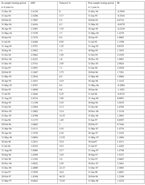
(11) Philosophical Transactions of the Royal Society , London, Series A 357 pp2039-2058 (1999) correlated with one-year information ratios then we know that portfolios selected on the basis of monthly testing are likely to remain good for much longer. Moreover if information ratios are consistently high and autocorrelated the preference criteria is stable over time. Highly autocorrelated information ratios show that if last months selection performed well, then next months selection is also likely to be good. In summary the preferences to be set include: a choice of fixed countries or a variable number of countries; constraints on country allocations that can be very flexible, such as 50% in the UK, or no short sales, or zero% in Japan; the length of lookback period for the model training; and any ‘plus’ over the EAFE if it is used as a benchmark. The diagnostics analysed include: in-sample stationarity tests for the tracking error (ADFs); monthly turnovers; and information ratios of post-sample performance over a testing period that is usually twelve months. Some examples of running the model in practice are now presented. Two different types of preferences are illustrated, one being a hedge portfolio and the other being an index tracking portfolio that is constrained to allow no short sales nor anything to be invested in Japan. They are presented purely as examples of the model backtesting and validation methodology and the illustrative portfolios are not intended as recommendations for practical use. The output in table 1 is for outperforming the EAFE index plus 2% per annum, with no short sales and no investment in Japan. Concentration/diversification preferences have been set for investment in up to 9 countries, and with a 4-year training period. The training output is given in the first three columns and the information ration (IR) for a post-sample testing period are reported to the right of the table. Each row in the table corresponds to one portfolio that has been chosen to be most highly cointegrated with the benchmark and also constrained to reflect the preferences set by the investor (in this case no short sales and none of the fund in Japan). The portfolios are rebalanced monthly or quarterly. The actual country allocations are not shown but see figure 2 for country allocations when WIES is used for the hedge fund.. 10 Because the residuals from ordinary least squares regression have zero mean. © Philosophical Transactions of the Royal Society of London. 11.

(12) Philosophical Transactions of the Royal Society , London, Series A 357 pp2039-2058 (1999) Table 1: Backtesting the preferences of no short sales and zero% in Japan In-sample training period. ADF. Turnover %. is 4-years to:. Post-sample testing period. IR. is 1-year to:. 31 Dec 93. -2.4159. 0. 31 Dec 94. -0.3954. 31 Jan 94. -2.4286. 13.7. 31 Jan 95. -0.3416. 28 Feb 94. -2.7067. 5.5. 28 Feb 95. 0.6716. 31 Mar 94. -2.4454. 6.3. 31 Mar 95. -0.0170. 30 Apr 94. -2.2907. 7.25. 30 Apr 95. -0.2239. 31 May 94. -2.7270. 3.7. 31 May 95. 1.4278. 30 Jun 94. -2.7474. 0.5. 30 Jun 95. 1.9063. 31 Jul 94. -2.6268. 0.95. 31 Jul 95. 1.1598. 31 Aug 94. -2.5351. 1.25. 31 Aug 95. 0.8325. 30 Sep 94. -2.5852. 1.9. 30 Sep 95. 1.7035. 31 Oct 94. -2.5662. 1.05. 31 Oct 95. 2.2529. 30 Nov 94. -2.4222. 1.8. 30 Nov 95. 1.9891. 31 Dec 94. -2.5741. 3.95. 31 Dec 95. 2.9024. 31 Jan 95. -2.4951. 7.1. 31 Jan 96. 2.2928. 28 Feb 95. -2.1847. 5.75. 28 Feb 96. 1.7201. 31 Mar 95. -2.2816. 6.5. 31 Mar 96. 1.9084. 30 Apr 95. -2.1831. 14.9. 30 Apr 96. 1.1432. 31 May 95. -1.8767. 8.4. 31 May 96. -0.2004. 30 Jun 95. -1.6848. 9.6. 30 Jun 96. -1.1051. 31 Jul 95. -2.2644. 5.25. 31 Jul 96. -0.8722. 31 Aug 95. -2.4214. 3.85. 31 Aug 96. 0.6893. 30 Sep 95. -3.1198. 5.45. 30 Sep 96. 1.0470. 31 Oct 95. -3.2954. 11.3. 31 Oct 96. 1.6794. 30 Nov 95. -3.3002. 13.4. 30 Nov 96. 1.3118. 31 Dec 95. -3.4768. 14.35. 31 Dec 96. 1.2892. 31 Jan 96. -3.1175. 1.65. 31 Jan 97. 0.6507. 28 Feb 96. -3.0682. 1. 28 Feb 97. 0.7446. 31 Mar 96. -3.4111. 5.55. 31 Mar 97. 1.4376. 30 Apr 96. -3.1976. 4.45. 30 Apr 97. 1.2103. 31 May 96. -3.0054. 13.55. 31 May 97. 1.1804. 30 Jun 96. -3.3631. 32.8. 30 Jun97. 1.4211. 31 Jul 96. -3.8745. 19.5. 31 Jul 97. 1.4205. 31 Aug 96. -3.4884. 15.7. 31 Aug 97. 1.4748. 30 Sep 96. -3.4569. 3.45. 30 Sep 97. 1.9127. 31 Oct 96. -3.1545. 3.4. 31 Oct 97. 2.0667. 30 Nov 96. -3.0922. 2.95. 30 Nov 97. 2.3661. 31 Dec 96. -2.4080. 22.15. 31 Dec 97. 2.3083. 31 Jan 97. -3.7039. 16.8. 31 Jan 98. 1.6091. 28 Feb 97. -1.8348. 46.55. 28 Feb 98. 1.2108. 31 Mar 97. -0.0642. 72.65. 31 Mar 98. 1.4225. © Philosophical Transactions of the Royal Society of London. 12.

(13) Philosophical Transactions of the Royal Society , London, Series A 357 pp2039-2058 (1999) 30 Apr 97. -0.9878. 8.3. 30 Apr 98. 1.5957. 31 May 97. -2.8355. 82.25. 31 May 98. 0.7172. 30 Jun97. -2.7019. 1.45. 30 Jun98. 0.7305. 31 Jul 97. -2.9622. 1.2. 31 Jul 98. 0.8534. 31 Aug 97. -3.0783. 1.75. 31 Aug 98. 1.2016. 30 Sep 97. -3.0405. 2.45. 31 Aug 98. 1.2284. 31 Oct 97. -3.0546. 1.6. 31 Aug 98. 1.5020. 30 Nov 97. -3.1603. 1.3. 31 Aug 98. 1.4473. 31 Dec 97. -2.9487. 2. 31 Aug 98. 0.5557. 31 Jan 98. -3.1410. 1.45. 31 Aug 98. 1.0104. 28 Feb 98. -3.1720. 0.1. 31 Aug 98. 1.8855. 31 Mar 98. -3.1131. 16.95. 31 Aug 98. 1.5793. 30 Apr 98. -3.1963. 2.2. 31 Aug 98. 0.7399. 31 May 98. -3.3073. 2.15. 31 Aug 98. 1.0287. 30 Jun98. -3.5255. 13.2. 31 Aug 98. 1.6629. 31 Jul 98. -3.7153. 12.55. 31 Aug 98. 1.2587. 31 Aug 98. -3.9901. 7.4. Notes: ADF = In-sample ADF statistic on tracking error stationary; IR = post-sample information ratio = mean tracking error/ std dev tracking error over the testing period, relative to the EAFE index; other diagnostics include autocorrelation of information ratios (0.7377) and crosscorrelation between 1-month and 1-year information ratios (0.4902).. A turnover index is first calculated as the sum of the absolute change in weights. This generally lies between 0 and 2.0, the latter occurring when there is 100% turnover in all assets (i.e. the entire portfolio moves out of one set of assets, then into another). The turnover percent reported in table 1 is simply this turnover index divided by 2 and expressed as a percentage. Turnovers are generally low, except between May 1996 and May 1997. But since the model is being constrained (much more constrained than for the hedging example given below) the turnovers are expected to be more variable. The ADFs show that insample tracking errors are stationary most of the time, but they are not always significant. One may conclude that the portfolios are weakly cointegrated with the EAFE plus 2%. What is encouraging is that cointegration is more significant towards the end of the sample, since all ADFs exceed –3 during 1998, and this is what matters when choosing the WIES parameters for current allocations. The post-sample information ratios are almost all positive. Looking at the IRs during 1998 one might reasonably expect a value of around 1 for a portfolio chosen on the basis of these preferences. It is possible to be reasonably confident of this because the IRs are highly autocorrelated (the autocorrelation coefficient is 0.7377). There is also a significant positive cross-correlation between the one-month and the twelve-month information ratios of 0.4902, showing that if a portfolio starts well during the first month it is likely to stay good. © Philosophical Transactions of the Royal Society of London. 13.

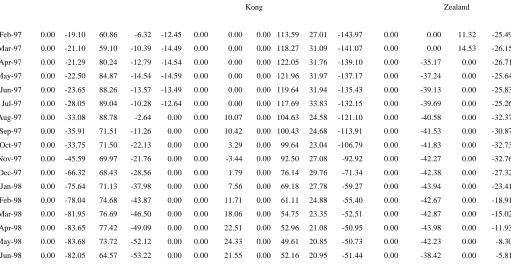
(14) Philosophical Transactions of the Royal Society , London, Series A 357 pp2039-2058 (1999) This combination of high autocorrelation and high cross-correlation in the information ratios is a great advantage, since it enables one-month ahead decisions to be made. The information ratios at the end of the training and testing output refer only to a few months of post-sample testing. Therefore one must seek a combination of high current IRs, high autocorrelation, and high cross correlation in IRs to predict that next month a portfolio chosen on the basis of these preferences will out-perform the EAFE index. The example of tracking EAFE plus 2%, no short sales and zero% in Japan has produced some promising results, but many other preferences would not. For example if we were to stipulate that 50% of the fund be allocated to the UK, it would be difficult to find portfolios that are highly cointegrated with the EAFE index. Tables 2 to 4 report results from using the model for a hedge. When the model is used in this way the problem becomes one of finding a long portfolio and a short portfolio that are highly cointegrated. Figures 2(a) and 2(b) illustrate the major long and short positions that would have obtained from using these preferences for the WIES hedge portfolio. Belgium, Ireland, Italy, Spain and the UK were all significantly long during this period, and Austria, Denmark, Japan and the Netherlands were short positions.. Table 2: WIES Hedge Fund Allocations. Date. Australia Austria Belgium Denmark Finland France Germany Hong. Ireland Italy. Japan. Malaysia Netherlands New. Kong. Norway. Zealand. Feb-97. 0.00. -19.10. 60.86. -6.32. -12.45. 0.00. 0.00. 0.00 113.59. 27.01. -143.97. 0.00. 0.00. 11.32. -25.49. Mar-97. 0.00. -21.10. 59.10. -10.39. -14.49. 0.00. 0.00. 0.00 118.27. 31.09. -141.07. 0.00. 0.00. 14.53. -26.15. Apr-97. 0.00. -21.29. 80.24. -12.79. -14.54. 0.00. 0.00. 0.00 122.05. 31.76. -139.10. 0.00. -35.17. 0.00. -26.71. May-97. 0.00. -22.50. 84.87. -14.54. -14.59. 0.00. 0.00. 0.00 121.96. 31.97. -137.17. 0.00. -37.24. 0.00. -25.64. Jun-97. 0.00. -23.65. 88.26. -13.57. -13.49. 0.00. 0.00. 0.00 119.64. 31.94. -135.43. 0.00. -39.13. 0.00. -25.83. Jul-97. 0.00. -28.05. 89.04. -10.28. -12.64. 0.00. 0.00. 0.00 117.69. 33.83. -132.15. 0.00. -39.69. 0.00. -25.26. Aug-97. 0.00. -33.08. 88.78. -2.64. 0.00. 0.00. 10.07. 0.00 104.63. 24.58. -121.10. 0.00. -40.58. 0.00. -32.37. Sep-97. 0.00. -35.91. 71.51. -11.26. 0.00. 0.00. 10.42. 0.00 100.43. 24.68. -113.91. 0.00. -41.53. 0.00. -30.87. Oct-97. 0.00. -33.75. 71.50. -22.13. 0.00. 0.00. 3.29. 0.00. 23.04. -106.79. 0.00. -41.83. 0.00. -32.73. Nov-97. 0.00. -45.59. 69.97. -21.76. 0.00. 0.00. -3.44. 0.00. 92.50. 27.08. -92.92. 0.00. -42.27. 0.00. -32.76. Dec-97. 0.00. -66.32. 68.43. -28.56. 0.00. 0.00. 1.79. 0.00. 76.14. 29.76. -71.34. 0.00. -42.38. 0.00. -27.32. Jan-98. 0.00. -75.64. 71.13. -37.98. 0.00. 0.00. 7.56. 0.00. 69.18. 27.78. -59.27. 0.00. -43.94. 0.00. -23.41. 99.64. Feb-98. 0.00. -78.04. 74.68. -43.87. 0.00. 0.00. 11.71. 0.00. 61.11. 24.88. -55.40. 0.00. -42.67. 0.00. -18.91. Mar-98. 0.00. -81.95. 76.69. -46.50. 0.00. 0.00. 18.06. 0.00. 54.75. 23.35. -52.51. 0.00. -42.87. 0.00. -15.02. Apr-98. 0.00. -83.65. 77.42. -49.09. 0.00. 0.00. 22.51. 0.00. 52.96. 21.08. -50.95. 0.00. -43.98. 0.00. -11.93. May-98. 0.00. -83.68. 73.72. -52.12. 0.00. 0.00. 24.33. 0.00. 49.61. 20.85. -50.73. 0.00. -42.23. 0.00. -8.30. Jun-98. 0.00. -82.05. 64.57. -53.22. 0.00. 0.00. 21.55. 0.00. 52.16. 20.95. -51.44. 0.00. -38.42. 0.00. -5.81. © Philosophical Transactions of the Royal Society of London. 14.

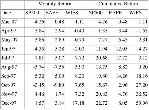
(15) Philosophical Transactions of the Royal Society , London, Series A 357 pp2039-2058 (1999) Jul-98. 0.00. -92.09. 52.66. -57.48. 0.00. 3.32. 29.53. 0.00. 21.62. 26.67. -46.35. 0.00. -29.62. 0.00. 6.16. Aug-98. 0.00. -84.61. 42.73. -37.16. 0.00. 0.00. 18.65. 0.00. 22.45. 25.24. -58.03. 8.55. -23.16. 0.00. -1.02. Sep-98. 0.00. -84.88. 0.00. -37.78. 0.00. 0.00. 19.52. 0.00. 39.05. 25.85. -58.24. 7.79. -7.51. 0.00. 1.30. Oct-98. 0.00. -71.67. 0.00. -50.08. 0.00. 0.00. 18.48. 0.00. 36.94. 0.00. -63.55. 0.00. -7.05. 0.00. 1.38. Nov-98. 0.00. -71.47. 0.00. -49.98. 0.00. 0.00. 18.67. 0.00. 35.51. 0.00. -63.98. 0.00. -6.76. 0.00. 2.53. Dec-98. 0.00. -71.04. 0.00. -51.72. 0.00. 0.00. 46.26. 0.00. 18.47. 0.00. -64.16. 0.00. -25.90. 0.00. 5.13. Jan-99. 0.00. -70.22. 0.00. -54.97. 0.00. 0.00. 47.00. 0.00. 16.83. 0.00. -63.72. 0.00. -25.28. 0.00. 9.74. Feb-99. 0.00. -70.11. 0.00. -55.28. 0.00. 0.00. 46.20. 0.00. 15.09. 0.00. -63.67. 0.00. -22.88. 0.00. 10.82. Notes: The coefficients are not normalized. For example in the last month they sum to 2.3, which implies a total leverage of 4.6 to 1. Table 3 shows monthly and cumulative returns that would have obtained from hedging with these preferences since March 1997, compared with those from tracking EAFE and S&P. These are some of the relevant results used during backtesting current preferences whilst training for the March 1999 allocations. Note that the returns that are reported during in-sample training are not the same as the realised returns from the managed portfolio. This is because the backtesting results are for just one preference set. In practice we are changing the optimal preferences each month, as different alphas, different training periods and different constraints on allocations appear more or less profitable during backtesting. Table 3: WIES Hedge Fund Returns. Monthly Return Date. SP500. EAFE. Cumulative Return. WIES. SP500. EAFE. WIES. Mar-97. -4.26. 0.48. -1.11. -4.26. 0.48. -1.11. Apr-97. 5.84. 2.94. -0.43. 1.33. 3.44. -1.53. May-97. 5.86. 2.89. -0.79. 7.27. 6.43. -2.31. Jun-97. 4.35. 5.28. -2.00. 11.94. 12.05. -4.27. Jul-97. 7.81. 5.07. 7.72. 20.68. 17.72. 3.12. Aug-97. -5.74. -7.56. 5.90. 13.75. 8.82. 9.20. Sep-97. 5.32. 5.00. 8.20. 19.80. 14.26. 18.16. Oct-97. -3.45. -9.89. 7.65. 15.67. 2.96. 27.20. Nov-97. 4.46. 1.74. 7.32. 20.83. 4.76. 36.52. Dec-97. 1.57. 3.14. 17.18. 22.72. 8.05. 59.96. © Philosophical Transactions of the Royal Society of London. 15.

(16) Philosophical Transactions of the Royal Society , London, Series A 357 pp2039-2058 (1999) Jan-98. 1.02. 4.66. 11.50. 23.98. 13.08. 78.36. Feb-98. 7.04. 5.55. 10.83. 32.70. 19.35. 97.67. Mar-98. 4.99. 4.99. 12.96. 39.33. 25.30. 123.29. Apr-98. 0.91. -0.69. 4.55. 40.59. 24.44. 133.46. May-98. -1.88. 0.94. -1.55. 37.95. 25.60. 129.84. Jun-98. 3.94. 1.13. 9.81. 43.39. 27.02. 152.39. Jul-98. -1.16. 1.57. 0.16. 41.72. 29.01. 152.80. Aug-98. -14.58. -14.48. 7.39. 21.06. 10.34. 171.49. Sep-98. -9.90. -6.82. 12.82. 9.08. 2.81. 206.28. Oct-98. 8.10. 6.15. -0.17. 17.91. 9.14. 205.77. Nov-98. 6.10. 7.63. 12.73. 25.10. 17.47. 244.71. Dec-98. 5.80. 1.24. 8.61. 32.36. 18.93. 274.38. Jan-99. 4.20. 1.27. 6.12. 37.92. 20.43. 297.31. Feb-99. -3.43. 0.91. -1.82. 33.19. 21.53. 290.09. 5. Concluding Remarks The extensive literature on cointegrated asset prices concerns both market efficiencies (e.g. spot and futures prices) and market inefficiencies (e.g. international equity markets). The innovation of cointegration is the direct application of non-stationary data, whereas most other methods employ stationary data from the outset. Cointegration arises naturally between a number of asset markets, and when cointegration is not taken into account there is a danger of mis-pricing, over-hedging and increased transaction costs. But any real common trends in the price time series, not merely statistical artefacts but consequences of economic and market forces, should be recognised by alternative statistical methodologies, such as principal component analysis. Cointegration, perhaps more than any other time series methodology, has been used pervasively and skilfully in econometrics, but there is a danger of forming false conclusions. There is sometimes a tendency for time series modelling to be lead by the technique, rather than any real relationship between the random variables in a multivariate system. But if the finding of a relationship between underlyings is not merely an artefact of the statistical methods used, and is really a result of market forces, then it should be corroborated by alternative statistical methods. It will ‘shine through’ a variety of statistical investigations, using a number of different methodologies. However if supposedly © Philosophical Transactions of the Royal Society of London. 16.

(17) Philosophical Transactions of the Royal Society , London, Series A 357 pp2039-2058 (1999) profitable relationships are only revealed when a finely tuned device such as cointegration is applied, then there is a good chance that the relationships are not sufficiently robust to be workable in practice. Cointegration provides a rigorous scheme that may be implemented with basic statistical techniques. Not numerical optimisation, not even maximum likelihood is necessary for the modeller to gain a crude insight to the common trends and error correction dynamics of a cointegrated system. And if no strong evidence is presented within a superficial investigation, it is unlikely that the trading P&Ls would support the use of the model. This paper has focussed on the use of cointegration for equity index tracking and hedging of international equity portfolios. From the above remarks it should be clear that however rigorous the modelling approach, it is the training and testing results on candidate portfolios that are paramount. It has been shown how such validation procedures may be put in place, and results have been presented for both hedging and index tracking.. Acknowledgement I am indebted to Wayne Weddington and Ian Giblin of Pennoyer Capital Management, New York, for providing the results used in section 4.. Bibliography Alexander, C. (1994) "History Debunked" RISK 7 No. 12 (1994) pp 59-63. Alexander, C.O. (1994) "Cofeatures in international bond and equity markets" University of Sussex Discussion Papers in Economics, No 94/1. Alexander, C.O. (1995) "Common volatility in the foreign exchange market" in Applied Financial Economics vol 5 No. 1 Alexander, C. (1995) "Cofeatures in international bond and equity markets" Mimeo Alexander, C. (1999) "Measuring Correlation in Energy Markets" Forthcoming in ‘Managing Energy Price Risk’ Second Edition, RISK Publications Alexander, C. and A. Johnson (1992) "Are foreign exchange markets really efficient?" Economics Letters 40 (1992) 449-453 Alexander, C. and A. Johnson (1994) "Dynamic Links" RISK 7:2 pp 56-61 Alexander, C. and R. Thillainathan (1996) "The Asian Connections" Emerging Markets Investor, 2:6 pp42-47 © Philosophical Transactions of the Royal Society of London. 17.

(18) Philosophical Transactions of the Royal Society , London, Series A 357 pp2039-2058 (1999) Baillie, R.T. and T. Bollerslev (1994a) "Cointegration, fractional cointegration, and exchange rate dynamics" Journal of Finance 49:2, June 1994, pp. 737-745. Beck, S.E. (1994) "Cointegration and market efficiency in commodities futures markets" Applied Economics 26:3, pp. 249-57 Bessler, D.A. and T. Covey (1991) "Cointegration - some results on cattle prices" Journal of Futures Markets 11:4 pp 461-474. Bopp A.E. and S. Sitzer (1987) "Are petroleum prices good predictors of cash value?" Journal of Futures Markets 7 pp 705-719. Bradley, M. and S. Lumpkin (1992) "The Treasury yield curve as a cointegrated system" Journal of Financial and Quantitative Analysis 27 pp 449-63. Brenner, R.J. and K.F. Kroner (1995) "Arbitrage, cointegration, and testing the unbiasedness hypothesis in financial markets" Journal of Financial and Quantitative Analysis 30:1, pp 23-42 Brenner, R.J., R.H. Harjes and K.F. Kroner (1996) “Another look at alternative models of the short term interest rate” Journal of Financial and Quantitative Analysis 31:1 pp85-108 Booth, G. and Y. Tse (1995) "Long Memory In Interest Rate Futures Markets: A Fractional Cointegration Analysis" Journal of Futures Markets 15:5 Campbell, J.Y., A.W. Lo and A.C. MacKinley (1997) The Econometrics of Financial Markets Princeton University Press. Cerchi, M. and A. Havenner (1988) "Cointegration and stock prices". Journal of Economic Dynamics and Control 12 pp 333-46. Chowdhury, A.R. (1991) "Futures market efficiency: evidence from cointegration tests" The Journal of Futures Markets 11:5 pp 577-89. Chelley-Steeley, P.L. and E.J. Pentecost (1994) "Stock market efficiency, the small firm effect and cointegration" Applied Financial Economics 4:6, December 1994, pp. 405-11 Choi, I. (1992) "Durbin-Hausmann tests for a unit root" Oxford Bulletin of Economics and Statistics 54:3 pp. 289-304. Chowdhury, A.R. (1991) "Futures market efficiency: evidence from cointegration tests" The Journal of Futures Markets 11:5 pp 577-89. John Wiley and Sons Inc., 1991. Cerchi, M. and A. Havenner (1988) "Cointegration and stock prices". Journal of Economic Dynamics and Control 12 pp 333-46. Clare, A.D., M. Maras and S.H. Thomas (1995) "The integration and efficiency of international bond markets" Journal of Business Finance and Accounting 22:2 pp. 313-22. Cochrane, J. H. (1991) "A critique of the application of unit root tests" Jour. Econ. Dynamics and Control 15 275-84. © Philosophical Transactions of the Royal Society of London. 18.

(19) Philosophical Transactions of the Royal Society , London, Series A 357 pp2039-2058 (1999) Coleman, M. (1990) "Cointegration-based tests of daily foreign exchange market efficiency". Economics Letters 32 pp 53-9. Corhay, C.A. Tourani Rad, J.-P. Urbain (1993) "Common stochastic trends in European stock markets." Economics Letters 42 pp. 385-90. Covey, T. and D.A. Bessler (1992) "Testing for Granger's full causality". The Review of Economics and Statistics pp 146-153. Dickey, D.A. and W.A. Fuller (1979) "Distribution of the estimates for autoregressive time series with a unit root" Journal of the American Statistical Association 74 pp. 427-9 Dickey, D.A., D.W. Jansen and D.L. Thornton (1991) "A primer on cointegration with an application to money and income". Federal Reserve Bank of St Louis March/April 1991 pp 58-78. Davidson, J., G. Madonia and P. Westaway (1994) "Modelling the UK gilt-edged market" Journal of Applied Econometrics 9:3, July-September 1994, pp. 231-53 DeGennaro, R.P., R.A. Kunkel and J. Lee (1994) "Modeling international long-term interest rates" Financial Review 29:4, November 1994, pp. 577-97 Duan, J-C and S. Pliska (1998) “Option valuation with cointegrated asset prices” Mimeo Dwyer, G.P. and M.S. Wallace (1992) "Cointegration and market efficiency" Journal of International Money and Finance 11 pp 318-327. Engle, R.F. and C.W.J. Granger (1987) "Co-integration and error correction: representation, estimation, and testing". Econometrica 55:2 pp 251-76. Engle, R.F. and B.S. Yoo (1987) "Forecasting and testing in cointegrated systems" Jour. Econometrics 35 143-159. Goodhart, C. (1988) "The foreign exchange market: a random walk with a dragging anchor". Economica 55 pp 437-60. Gourieroux, C., A. Monfort and E. Renault (1991) "A general framework for factor models". Institut National de la Statistique et des Etudes Economiques no. 9107. Granger, C.W.J. (1988) "Some recent developments on a concept of causality". Jour. Econometrics 39, pp. 199 - 211. Hakkio, C.S. and M. Rush (1989) "Market efficiency and cointegration: an application to the sterling and Deutschmark exchange markets". Journal of International Money and Finance 8 pp 75-88. Hall, A.D., H.M. Anderson and C.W.J. Granger (1992) "A cointegration analysis of Treasury bill yields". The Review of Economics and Statistics pp 116-26. Hamilton, J.D. (1994) Time Series Analysis Princeton University Press. © Philosophical Transactions of the Royal Society of London. 19.

(20) Philosophical Transactions of the Royal Society , London, Series A 357 pp2039-2058 (1999) Harris, F. deB., T. H. McInish, G. L. Shoesmith and R. A. Wood (1995) "Cointegration, Error Correction, And Price Discovery On Informationally Linked Security Markets" Journal of Financial and Quantitative Analysis 30:4 Hendry, D.F. (1986) "Econometric modelling with cointegrated variables: an overview". Oxford Bulletin of Economics and Statistics 48:3 pp 201-12. Hendry, D.F. (1995) Dynamic Econometrics Oxford University Press Johansen, S (1988) "Statistical analysis of cointegration vectors". Journal of Economic Dynamics and Control 12 pp 231-54. Johansen, S. and K. Juselius (1990) "Maximum likelihood estimation and inference on cointegration with applications to the demand for money". Oxford Bulletin of Economics and Statistics 52:2 pp 169-210. Karfakis, C.J. and D.M. Moschos (1990) "Interest rate linkages within the European monetary system: a time series analysis". Journal of Money, Credit, and Banking 22:3 (August 1990), Ohio State University Press, pp 388-94. Kasa, K. (1992) "Common stochastic trends in international stock markets" Journal of Monetary Economics 29, pp. 95-124 Khoury N.T. and P. Yourougou (1991) "The informational content of the basis: evidence from Canadian barley, oats and canola futures markets" Journal of Futures Markets 11:1 pp. 69-80 Lai, K.S. and M. Lai (1991) "A cointegration test for market efficiency" Journal of Futures Markets 11 (1991) pp 567-76. Lee, T-H (1994) "Spread and volatility in spot and forward exchange rates" Journal of International Money and Finance 13:3, June 1994, pp. 375-83. Lo, A.W. and A.Craig MacKinlay (1988) "Stock Market prices do not follow random walks: evidence from a simple specification test." Review of Financial Studies 1:1 pp 41-66. Masih, R. (1997) “Cointegration of markets since the ’87 crash” Quarterly Review of Economics and Finance 37:4 MacDonald, R. and M. Taylor (1988) "Metals prices, efficiency and cointegration: some evidence from the London Metal Exchange" Bulletin of Economic Research 40 (1988) pp. 235-9. Macdonald, R. and M.P. Taylor (1994) "The monetary model of the exchange rate: Long-run relationships, short-run dynamics and how to beat a random walk" Journal of International Money and Finance 13:3, June 1994, pp. 276-90 Mackinnon, J.G. (1994) "Approximate asymptotic distribution functions for unit-root and cointegration tests" Journal of Business Economics and Statistics 12:2, April 1994, pp. 167-176. © Philosophical Transactions of the Royal Society of London. 20.

(21) Philosophical Transactions of the Royal Society , London, Series A 357 pp2039-2058 (1999) Nelson, C.R. and C.I. Plosser (1982) "Trends and random walks in macroeconomic time series". Journal of Monetary Economics 10 pp 139-62. Nieuwland, Frederick G.M., W. Verschoor, F.C. Willen and C.C.P. Wolff (1994) "Stochastic trends and jumps in EMS exchange rates" Journal of International Money and Finance 13:6, December 1994, pp. 669-727 Nugent, J (1990) "Further evidence of forward exchange market efficiency: an application of cointegration using German and U.K. data" Economic and Social Reviews, 22 pp. 35-42. Phillips, P.C.B. and P. Perron (1988) "Testing for a unit root in time series regressions" Biometrika 75 pp. 335-46 Pindyck, R.S. and J.J. Rothemberg (1992) "The comovement of stock prices." Quarterly Journal of Economics pp. 1073-1103. Proietti, T. (1997) “Short-run dynamics in cointegrated systems” Oxford Bulletin of Economics and Statistics 59:3 Schroeder , T C and B.K. Goodwin (1991) "Price discovery and cointegration for live hogs" Journal of Futures Markets 11 : 6 pp685-696 Schwarz, T.V. and F.E. Laatsch (1991) "Dynamic efficiency and price discovery leadership in stock index cash and futures market" Journal of Futures Markets 11 : 6 pp669-684. Schwarz, T.V. and A.C. Szakmary (1994) "Price discovery in petroleum markets: arbitrage, cointegration, and the time interval of analysis". Journal of Fututres Markets 14:2, pp 147-167. Schmidt, P. and P.C.B. Phillips (1992) "LM tests for a unit root in the presence of deterministic trends" Oxford Bulletin of Economics and Statistics 54: 3 pp. 257-288. Smith, K.L., J. Brocato and J.E. Rogers (1993) "Regularities in the data between major equity markets: evidence from Granger causality tests". Applied Financial Economics 3 55-60. Wang, G. H. K. and J. Yau (1994) "A Time Series Approach To Testing For Market Linkage: Unit Root And Cointegration Tests" Journal of Futures Markets 14:4. © Philosophical Transactions of the Royal Society of London. 21.

(22) Philosophical Transactions of the Royal Society , London, Series A 357 pp2039-2058 (1999). Figure 1(a): NLG a n d D E M returns Dutch Guilder Deutsche Mark. Figure 1(b): NLG a n d D E M rates Dutch Guilder Deutsche Mark. © Philosophical Transactions of the Royal Society of London. 22.

(23) Philosophical Transactions of the Royal Society , London, Series A 357 pp2039-2058 (1999) F ig u r e 1 ( c ) : N L G ' P l u s ' v s . D E M Deutsche Mark Guilder 'Plus'. © Philosophical Transactions of the Royal Society of London. 23.

(24)

No results found