45 *Corresponding author
Email address: [email protected]
A method for detecting bubbles in two-phase gas-liquid flow
P. Hanafizadeh*, A. Sattari, S. E. Hosseinidoost, M. Molaei and M. Ashjaee
Center of Excellence in Design and Optimization of Energy Systems, School of Mechanical Engineering, College of Engineering, University of Tehran, Tehran, Iran
Article info: Abstract
Bubble detecting bubble has been a basic issue in two-phase flow systems. In this paper, a new method for measuring the frequency of bubble formation is presented. For this purpose, an electronic device is designed and constructed to work based on a change in intensity of the laser beam. Continues light beam is embedded just above the needle, which is received by a phototransistor. When bubbles go through the light beam, they make a deviation on it and change its intensity. So, the electrical resistance between two bases of phototransistor changes, and this variation is sensed by an electronic board. Based on the number of interruption and duration time, the frequency of bubble formation is be calculated. Liquid and gas phases in the present work are water and air, respectively. Tests are performed in constant liquid height (60 mm above the needle), constant needle diameter (1.6 mm), and gas flow rates between 50 to 1200 ml/hr. Also, three other methods are utilized to measure the bubble frequency: image processing (IP), numerical modeling, and theoretical model. Results show that with an increase in the flow rate of the gas phase, the frequency of formation increases approximately in a linear manner. Validation of methods with IP method shows that the new device has very good accuracy for measuring bubble formation frequency. So because of the simplicity of using and low cost, it can be a superseded method of image processing.
Received: 29/04/2017 Accepted: 05/12/2018 Online: 05/12/2018 Keywords:
Two-phase flow, Bubble,
Frequency of formation, Electronic device, Image processing.
Nomenclature
a Acceleration
A Projection area of bubble D Diameter of bubble
f Frequency of bubble formation FB Buoyancy force
FD Drag force
FV Virtual mass force
F Surface tension force G Gravity force m Bubble mass
ṁ Mass transfer
P Circumference of the needle Q Volumetric flow rate Re Reynolds number
u Velocity
Uf Volume flux through the face
V Volume of bubble VC Volume of cell
Greek symbols
q Volume fraction
Contact angle of bubble
Density
Interfacial tension Subscripts
46
1. Introduction
The dynamic of bubble formation has a major role in diverse applications related to scattering of gas bubbles in liquids such as water treatment, chemical reactors, metallurgy, and medical. Also, it is an important subject in the context of two-phase heat transfer [1-3]. This phenomenon is affected by different parameters such as the equivalent diameter of injection, the geometry of injection, gas flow rate, liquid and gas physical properties, the height of the liquid column, and wettability.
On the terrain of bubble formation in various conditions, abundant works have been done. For instance, Davidson and Amick [4] worked on the formation of gas bubbles at horizontal orifices. Influence of different parameters was examined on the formation of bubbles such as the diameter of the orifice, the volume of the chamber, and physical properties. In another research, Ramakrishnan et al. [5] studied bubble formation under constant flow conditions and proposed a model based on two-step mechanism of bubble formation. Also, Akita and Yoshida [6] investigated bubble size, interfacial area, and liquid-phase mass transfer coefficient in bubble columns. They presented dimensionless correlations for the average bubble size. In another paper, Sada et al. [7] conducted a research on bubble formation in a flowing liquid. They found that the bubble size in the flowing liquid decreases with increasing superficial liquid velocity and decreasing gas flow rate. Furthermore, Tsuge and Hibino [8] investigated bubble formation from an orifice submerged in liquids. The effects of various factors, such as orifice diameter, gas physical properties and gas chamber on the volume of bubbles were explored. Also, Kim et al. [9] developed a theoretical model for bubble and drop formation in flowing liquids in microgravity using a force balance. They found that the bubbles are detached from the nozzle only by the liquid flow drag. Byakova et al. [10] examined the influence of wetting conditions on bubble formation at the orifice in an inviscid liquid mechanism of bubble evolution. They concluded that the influence of operating variables on the formation of the bubble is different under various wetting
conditions. Corchero et al. [11] performed experimental investigations on the effects of wetting conditions and flow rate on bubble formation at orifices. Also, a simple model of the bubble shape at detachment was proposed that gives results in good agreement with those obtained from experiments done at small flow rates. Qu and Qiu [12] worked on bubble dynamics under a horizontal microheater array. They studied the effects of Marangoni, buoyancy, and drag forces on the bubble dynamic phenomena using experimental data. In another work, Ohta et al. [13] conducted a computational study on the dynamic motion of a bubble rising in Carreau model fluids. They utilized the Volume of Fluid (VOF) numerical model in order to simulate the mechanism of bubble formation. They discussed bubble rise motion in shear-thinning fluids in terms of the effective viscosity, and the effective Reynolds and Morton numbers. In another work, Vafaei et al. [14] investigated the bubble growth rate from needle nozzles. They realized that the bubble volume expansion rate follows a cyclic behavior for the substrate nozzles while it shows a smooth decrease after an initial increase for the needle nozzles. Finally, Di Bari and Robinson [15] conducted an experimental study of gas injected bubble growth from submerged orifices. The quasi-static growth and departure characteristics showed little dependence on the growth rate while having a notable dependence on the orifice size.
47 although it is not an accurate method nowise.
Another method for measuring bubble formation frequency utilized by some researches is the use of different kinds of probes, like optical and conductivity probes, which are high costs as high-speed cameras. For instance, Harvey et al. [21] measured vapor bubble using image analysis. They presented a method of computer image analysis to determine flow quantities of a single vapor bubble as it evolves near a rigid boundary. Also, Davidson et al. [22] measured the frequency of bubble formation by stroboscopic illumination. By experimental investigations, they concluded that the frequency of bubble formation decreases with increasing orifice diameter. In another paper, Lguchi et al. [23] investigated the effects of cross-flow on the frequency of bubble formation from a single-hole nozzle using a high-speed camera. They compared the frequency of bubble formation in a rotating bubble bath with that of a stationary one and concluded that before a critical value of cross-flow velocity, the ratio of frequencies is unity and after that, it changes in a complex manner. In another research, Badam et al. [24] perused regimes of bubble formation experimentally utilizing a high-speed camera. They found that at high gas flow rates, bubble formation frequency remains constant and bubble volume is almost independent of surface tension. Also, Zhang et al. [25] worked on drag coefficient on bubble rising. They calculated the volume of the bubble by dividing the gas flow rate to bubble formation frequency. They measured the frequency of bubble formation by counting the bubbles generated in a time interval. In addition, Hanafizadeh et al. [26–28] in a series of studies investigated the formation, growth, and detachment of gas bubbles produced from a submerged needle in water using a high-speed camera. They concluded that bubble formation frequency strongly depends on the contact angle and the surface tension, and it increases with increasing gas flow rate.
In the current work, a new method for calculating bubble frequency is presented. In this method, an electronic device is designed and constructed to work based on changes in the intensity of the light beam. Also, the frequency is measured using image processing, numerical,
and theoretical methods. Finally, errors of methods are computed in comparison with the IP method (because this technique has been widely used in the literature) and the most accurate method is specified.
2. Experimental apparatus
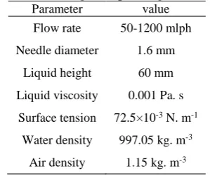
Schematic view of the experimental setup of the present work is shown in Fig. 1. The experimental system consists of a syringe pump, a square column, a standard circular needle with 1.6 mm diameter, a light source, a high-speed video camera (1200 fps), and a frequency meter device. For photographic observations, the square column made from PMMA with a dimensions of 100 mm × 100 mm × 300 mm and open to the atmosphere at the top is utilized ((1) in Fig. 1). The height of the liquid is constant and equal to 60 mm above the needle. The camera records movies with 1200 fps and 336×96 pixels ((4) in Fig. 1) and sends them to the computer ((6) in Fig. 1) for image processing. In order to wipe out reflections, one800 W halogen lamp is placed just in front of the camera ((5) in Fig. 1). The injection system located at the bottom of the column is composed of a needle ((2) in Fig. 1) as a source of injection joint to an automatically controlled syringe pump ((3) in Fig. 1). The syringe pump is filled with air, and the flow rate range is between 50 to 1200 ml/hr. The frequency meter system contains a 200 mW laser ((9) in Fig. 1), a phototransistor ((7 in Fig. 1) and an electronic board ((8) in Fig. 1) for processing data. The range of operating conditions are given in Table 1 (physical properties are computed at 20oC).
Table 1. The range of operating conditions.
Parameter value Flow rate 50-1200 mlph Needle diameter 1.6 mm
Liquid height 60 mm Liquid viscosity 0.001 Pa. s
Surface tension 72.5×10⁻³ N. m-1
Water density 997.05 kg. m-3
48
Fig. 1.Schematic view of the experimental setup; (1) bubble column, (2) injection needle, (3) syringe pump, (4) high-speed video camera, (5) light source, (6) computer, (7) phototransistor, (8) electronic board, and (9) laser.
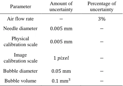
When the variables are the values of experimental measurements, they have uncertainties due to measurement limitations. For the present research, the uncertainties of measured data are given in Table 2. In this table, based on the accuracy of the measuring instruments, the precision of the major parameters is reported. Moreover, based on the analysis of the uncertainty studied by Lazar et al. [29], the uncertainty of the bubble diameter and volume are computed.
Table 2. The uncertainty of the experimentally measured variables.
Parameter Amount of uncertainty
Percentage of uncertainty Air flow rate − 3%
Needle diameter 0.005 mm −
Physical
calibration scale 0.005 mm − Image
calibration scale 1 𝑝𝑖𝑥𝑒𝑙 − Bubble diameter 0.05 mm −
Bubble volume 0.1 mm3 −
3. Methodology
As mentioned before, four methods are utilized in this project to measure the frequency of bubble formation; image processing (IP),
frequency device, numerical modeling, and theoretical model. Each of this methods is explained except the IP method. For the detail of the IP method see Ref. [30].
3.1.Frequency measurement unit
In order to measure the frequency of bubble formation, a continuous light beam is embedded just above the needle, which is received by a phototransistor as shown in Fig. 1. When bubbles go through this light beam, make a deviation on that and change the intensity of light. So, the electrical resistance between two bases of phototransistor changes and this variation is sensed by an electronic board. According to the number of interruption and duration time, the frequency of bubble formation can be calculated. Fig. 2(a) and (b) shows the continuous and interrupted light beam by rising bubble, respectively.
(a) (b)
Fig. 2. (a) Continuous light beam and (b) interrupted light beam by the bubble.
49 Fig. 3 illustrates the measured voltage versus
time for different flow rates. The peaks of the charts are related to the moments in which the laser beam is interrupted by rising bubbles. Furthermore, it is clear that with increasing gas flow rate, the distance between peaks gets closer to each other which means the frequency of formation increases. This can be justified by this fact that with increasing gas flow rate, the upward forces acting upon rising bubble dominates downward forces and resulted in a lower time of formation.
(a)
(b)
(c)
(d)
Fig. 3. Fluctuation time for (a) 400 (b) 600 (c) 800 (d) 1000 ml/hr flow rate with frequency device.
3.2.Theoretical modeling
To compare the obtained results from the presented method, a theoretical model based on force balancing is also used in this paper. Assumptions of force balancing in the theoretical modeling are as follows:
All properties of fluids are assumed to be constant and are computed at room temperature.
Bubble growth happens adiabatically and axisymmetric.
The liquid is quiescent, so the liquid trust force is not considered.
The pressure of the gas is uniform within the bubble, and the influence of gas viscosity is negligible due to the high Reynolds number.
Gas momentum force is negligible compared with other forces acting on the bubble.
As the thickness of the orifice is negligible, in comparison with the equivalent diameters of it, the contact line between the needle and bubble is considered to be fixed to the inner rim of the needle.
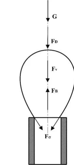
Based on the second law of Newton and the above assumptions, and by considering Fig. 4, the force balance equation can be written as follow:
𝑚𝑎 = 𝐹𝐵+ 𝐹𝜎+ 𝐹𝐷+ 𝐹𝑉+ 𝐺 (1)
where FB, F, FD, FV, and G are buoyancy,
surface tension, drag, virtual mass, and gravity forces, respectively [31]. So force balance can be written as follow:
𝑚𝑔𝑎𝑦= (𝜌𝑙− 𝜌𝑔)𝑔𝑉𝑔− 𝜎𝑃𝑠𝑖𝑛𝜃
−1 2𝜌𝑙𝐶𝐷𝑢𝑔
2𝐴
−1 2𝑉𝑔𝜌𝑙𝑎𝑦
(2)
By simplifying the above equation, the final equation for bubble volume is as follow:
𝑉𝑔=
𝜌𝑙𝐶𝐷𝑢𝑔2𝐴 + 2𝜎𝑃𝑠𝑖𝑛𝜃 2(𝜌𝑙− 𝜌𝑔)𝑔 − (𝜌𝑙+ 2𝜌𝑔)𝑎𝑦
(3)
where:
𝜌𝑙: Density of liquid phase 𝜌𝑔: Density of gas phase
50
𝐶𝐷: Drag coefficient (that is dependent on Reynolds number)
𝑢𝑔: Gas velocity
𝑆: Reference area of the bubble (that is equal to 𝜋 𝐷2⁄4)
𝑎𝑦: Acceleration of rising bubble
𝜎: The surface tension between water and air 𝜃: Contact angle of the bubble at the detachment 𝑃: Circumference of the injection needle
For Reynolds numbers between 20 and 260, 𝐶𝐷 can be calculated by Ishii equation (Eq. (4)) [32]:
𝐶𝐷 = 24
𝑅𝑒(1 + 0.1𝑅𝑒
0.75) (4)
Finally, the frequency of bubble formation can easily be computed using the flow rate as below:
𝑓 =𝑄 𝑉𝑔
= 𝑄 ×2(𝜌𝑙− 𝜌𝑔)𝑔 − (𝜌𝑙+ 2𝜌𝑔)𝑎𝑦 𝜌𝑙𝐶𝐷𝑢𝑔2𝐴 + 2𝜎𝑃𝑠𝑖𝑛𝜃
(5)
where 𝑄 is the flow rate of the dispersed phase and 𝑉𝑔 is the volume of the bubble at the detachment.
In this research, velocity and also its changes are very small at detachment, so drag force and acceleration are negligible. Therefore, Eqs. (3) and (5) are simplified as below:
𝑉𝑔=
2𝜎𝑃𝑠𝑖𝑛𝜃 2(𝜌𝑙− 𝜌𝑔)𝑔
(6)
𝑓 =𝑄 𝑉𝑔
= 𝑄 ×2(𝜌𝑙− 𝜌𝑔)𝑔
2𝜎𝑃𝑠𝑖𝑛𝜃 (7)
Q in the above formula is obtained from the syringe pump that plays both roles of injection and controlling flow. l, g and are physical properties of the liquid and gas phase and are measured at 20oC. P is the circumferenceof the circular needle that can easily be computed from the below equation:
𝑃 = 𝜋𝐷 (8)
where D is the diameter of the needle. Finally, is the contact angle of the bubble at detachment that is computed using experimental data processed by the image processing method. So, a theoretical method is dependent on experimental data due to the contact angle.
Fig. 4. Schematic force balance in the current study.
3.3.Numerical modeling
51 fraction in the cell is marked as 𝛼𝑞, then three
conditions may happen [33]:
𝛼𝑞= 0: The cell is empty (of the 𝑞𝑡ℎ fluid).
𝛼𝑞= 1: The cell is full (of the 𝑞𝑡ℎ fluid).
0 < 𝛼𝑞 < 1: The cell contains the interface between the 𝑞𝑡ℎ fluid and one or more other fluids.
Suitable properties and variables are
determined for each control volume within
the domain based on the local value of 𝛼
𝑞.
3.3.1. Volume fraction equation
Exploring the interface(s) between the phases is accomplished by solving the continuity equation for the volume fraction of one (or more) of the phases. For the 𝑞𝑡ℎ phase, this equation is as follows [33]:
1 𝜌𝑞
[𝜕
𝜕𝑡(𝛼𝑞𝜌𝑞) + ∇ ∙ (𝛼𝑞𝜌𝑞𝜈⃗𝑞)
= 𝑆𝛼𝑞
+ ∑(𝑚̇𝑝𝑞− 𝑚̇𝑞𝑝) 𝑛
𝑝=1
]
(9)
where 𝑚̇𝑝𝑞 is the mass transfer from phase 𝑞 to phase 𝑝 and 𝑚̇𝑝𝑞 is the mass transfer from phase 𝑝 to phase 𝑞.
The volume fraction equation is not solved for the primary phase, while the primary-phase volume fraction is computed based on the following constraint [33]:
∑ 𝛼𝑞 𝑛
𝑞=1
= 1 (10)
The volume fraction equation can be solved through implicit or explicit time discretization. Because of the faster convergence rate of the explicit method, using this method is preferred in this paper.
3.3.2. The explicit scheme
The formulation of this method can be defined as below [33]:
𝛼𝑞𝑛+1𝜌𝑞𝑛+1− 𝛼𝑞𝑛𝜌𝑞𝑛
Δ𝑡 𝑉𝑐
+ ∑(𝜌𝑞𝑈𝑓𝑛𝛼𝑞,𝑓𝑛 ) 𝑓
= [𝑆𝛼𝑞
+ ∑(𝑚̇𝑝𝑞− 𝑚̇𝑞𝑝) 𝑛
𝑝=1
] 𝑉
(11)
where 𝑛 + 1 is the index for new (current) time step, 𝑛 is the index for previous time step, 𝛼𝑓,𝑞 is the face value of the 𝑞𝑡ℎ volume fraction, 𝑉𝑐 is the volume of the cell, and 𝑈𝑓 is the volume flux through the face, based on normal velocity. This formulation does not require the iterative solution of the transport equation during each time step.
3.3.3. Momentum equation
Throughout the domain, a single momentum equation is solved, and the resulting velocity field is shared between the phases. The momentum equation is dependent on the volume fractions of all phases through the properties of 𝜌 and 𝜇 as below[33]:
𝜕
𝜕𝑡(𝜌𝜈⃗) + ∇. (𝜌𝜈⃗𝜈⃗) = −∇𝑝
+ ∇. [𝜇(∇𝜈⃗ + ∇𝜈⃗𝑇)] + 𝜌𝑔⃗ + 𝐹⃗
(12)
It should be noted that both phases in the present study are considered to be incompressible. In cases with large velocity differences between the phases, the accuracy of the velocities calculated near the interface can be adversely affected, and this is one restriction of the shared-field approximation.
52
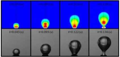
contribution of downward forces. In next stage, a bubble is formed with low velocity, so upward and downward forces are approximately. In the final stage, upward forces dominate downward ones, and an acceleration movement happens. Also, as shown in this figure, the numerical method can predict the sequence of the bubble formation pretty well and has a good agreement with the real bubble formation process.
Fig. 5. Comparison of bubble formation sequence between numerical and experimental data for 800 ml/hr flow rate.
In order to calculate the bubble frequency formation using a numerical method, contours of volume fraction are gathered as picture files and then by image processing method, the frequency is computed.
4. Results and discussions
Results are divided into two sections: results of frequency device, as the main approach of the current paper, and those of other methods. In the first section, details of gathering processing data by frequency and the device are explained and presented. In the next section, the results of other methods are just presented.
The results gathered by the frequency device are shown in Fig. 4. As shown in these diagrams, ADC0's number versus time can be seen. By interrupting the light beam by bubbles, the ADC0's number reaches approximately 250. So by the number of peaks in diagrams and duration time of them, the frequency of bubble formation can easily be computed. Also, it is clear from the figure that with increasing gas flow rate, the number of picks in a certain time increasesmeaning that the frequency of formation increases. The results of methods
applied to measure the frequency of formation for different flow rates are shown in Table 3.
Table 2. Comparison of frequency results of different methods.
Flow rate (ml/hr)
Image processing
(Hz)
Frequency device
(Hz)
Numerical (Hz)
Theoretical (Hz) 50 0.4836 0.4754 0.7097 0.4886 100 1.0093 0.9894 1.4493 0.9491 200 1.8519 1.8186 2.0534 1.7908 400 3.4823 3.4448 3.5714 3.5218 600 5.2131 5.1570 5.6818 5.2570 800 7.0468 6.9655 6.8966 6.9382 1000 8.4906 8.3219 8.8757 8.6539 1200 10.8768 10.6704 10.1371 10.3837
As the IP technique has been widely used in the literature, the obtained results of the other methods are compared with this method. The calculated percentage of errors are tabulated in Table 4. The presented errors are computed according to the following equation:
%𝐸𝑟𝑟𝑜𝑟 =𝑓𝐼𝑃− 𝑓𝑖 𝑓𝐼𝑃
× 100 (13)
where 𝑓𝐼𝑃 and 𝑓𝑖 are the frequency of bubble formation measured from the IP and other methods, respectively.
Table 4. Errors of different methods in comparison with the IP method.
Flow rate (ml/hr)
Frequency device
(%)
Numerical (%)
Theoretical (%) 50 1.6956 46.7535 1.0339 100 1.9717 43.5946 5.9645 200 1.7982 10.8807 3.2993 400 1.0769 2.5587 1.1343 600 1.0761 8.9908 0.8421 800 1.1537 2.1315 1.5411 1000 1.9869 4.5356 1.9233 1200 1.8976 6.8007 4.5335
53 tension forces. It demonstrates assumptions for
deriving Eq. (7) are admissible. Finally, as shown in Table 4, the numerical method has the lowest accuracy, especially at high flow rates, but it is not originated from the actual results so far. One major reason of this low accuracy is the difficulty of modeling the interface of gas and liquid phases in the numerical model due to the numerical diffusion and the need for a high grid resolution, which results in a non-sharp interface.
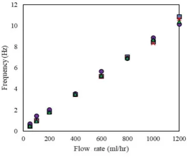
Fig. 6 shows the frequency of bubble formation versus flow rate for four mentioned methods. As can be seen, the frequency of formation increases approximately linearly with increasing gas flow rate. It can be justified with this fact that increasing gas flow rate tends to the increase in momentum of the bubble. As a result, faster detachment is obtained in higher frequency of formation at higher flow rates. As shown in Fig. 6, the frequency device method has the most precision between two other methods (numerical and theory model). Also, results confirm the previous researches which by increasing the flow rate of gas injection, the frequency of bubble formation increases.
Fig. 6. Frequency of bubble formation versus flow rate for four methods.
Fig. 7 illustrates the diagram of IP versus frequency device method. The average root mean square error between the results of frequency device and image processing method is less than 2%showing that the device has good accuracy.
Fig. 7. Frequency of bubble formation from IP method versus frequency device method.
To put the accuracy of this method into perspective, two of the most important correlations presented for calculating the volume of the bubble at the detachment in constant flow condition are taken into account. Then using Eq. (7), the frequency of formation for each correlation is calculated and compared with the experimental data of the present study, and shown in Fig. 8. As can be seen, both correlations presented by Gaddis and Vogelpohl [34] and Jamialahmadi et al. [35] have good agreement with the experimental data, especially at relatively low flow rates. The most error between the experimental data and Gaddis and Vogelpohl correlation is about 14%, while this error for Jamialahmadi et al. correlation is about 18%.
54
5. Conclusions
In this paper, an electronic device is designed and constructed to measure the frequency of bubble formation based on a change in intensity of the laser beam. The main features of the device are:
High accuracy despite the low cost
The ability of momentary measuring of bubble or any other object frequency for industrial applications
Simple electronic circuit
So simple to use
The accuracy of this new method is compared with other common methods: IP, numerical and theoretical modeling. Results show that this method has very good accuracy. The average root mean square error between the results of frequency device and image processing method is less than 2%. So it can be used as an alternative method of image processing in many applications.
References
[1] M. G. Reddy, M. V. V. N. L. S. Rani, K. G. Kumar, and B. C. Prasannakumara, “Cattaneo–Christov heat flux and non-uniform heat-source/sink impacts on radiative Oldroyd-B two-phase flow across a cone/wedge,” J. Brazilian Soc. Mech. Sci. Eng., Vol. 40, No. 2, p. 95, (2018).
[2] M. G. Reddy and O. D. Makinde, “Magnetohydrodynamic peristaltic transport of Jeffrey nanofluid in an asymmetric channel,” J. Mol. Liq., Vol. 223, pp. 1242-1248, (2016).
[3] M. Gnaneswara Reddy and N. Sandeep, “Free convective heat and mass transfer of magnetic bio-convective flow caused by a rotating cone and plate in the presence of nonlinear thermal radiation and cross diffusion,” J. Comput. Appl. Res. Mech. Eng., Vol. 7, No. 1, pp. 1-21, (2017). [4] L. Davidson and J. Erwin H. Amick,
“Formation of Gas Bubbles at Submerged Orifices,” AIChE J., Vol. 5, No. 3, pp. 319-324, (1956).
[5] S. Ramakrishnan, R. Kumar, and N. R. Kuloor, “Studies in bubble formation—I bubble formation under constant flow conditions,” Chem. Eng. Sci., Vol. 24, No. 4, pp. 731-747, (1969).
[6] K. Akita and F. Yoshida, “Gas Holdup and Volumetric Mass Transfer Coefficient in Bubble Columns. Effects of Liquid Properties,” Ind. Eng. Chem. Process Des. Dev., Vol. 12, No. 1, pp. 76-80, (1973). [7] E. Sada, A. Yasunzshz, S. Katoh, and M.
Nishioka, “Bubble Formation in Flowing Liquid,” Can. J. Chem. Eng., Vol. 56, No. 6, pp. 669-672, (1978).
[8] H. Tsuge and S.-I. Hibino, “Bubble Formation From an Orifice Submerged in Liquids,” Gordon Breach. Sci. Publ. Inc., Vol. 22, pp. 63-79, (1983).
[9] I. Kim, Y. Kamotani, and S. Ostrach, “Modeling bubble and drop formation in flowing liquids in microgravity,” AIChE J., Vol. 40, No. 1, pp. 19-28, (1994). [10] A. . Byakova, S. . Gnyloskurenko, T.
Nakamura, and O. . Raychenko, “Influence of wetting conditions on bubble formation at orifice in an inviscid liquid Mechanism of Bubble Evolution,”
Colloids Surfaces A Physicochem. Eng. Asp., Vol. 229, No. 1-3, pp. 19-32, (2003). [11] G. Corchero, a. Medina, and F. J. Higuera, “Effect of wetting conditions and flow rate on bubble formation at orifices submerged in water,” Colloids Surfaces A Physicochem. Eng. Asp., Vol. 290, No. 1-3, pp. 41-49, (2006).
[12] X. Qu and H. Qiu, “Bubble dynamics under a horizontal micro heater array,” J. Micromechanics Microengineering, Vol. 19, No. 9, p. 095008, (2009).
[13] M. Ohta, Y. Yoshida, and M. Sussman, “A computational study of the dynamic motion of a bubble rising in Carreau model fluids,” Fluid Dyn. Res., Vol. 42, No. 2, p. 025501, (2010).
[14] S. Vafaei, P. Angeli, and D. Wen, “Bubble growth rate from stainless steel substrate and needle nozzles,” Colloids Surfaces A Physicochem. Eng. Asp., Vol. 384, No. 1-3, pp. 240-247, (2011).
55 “Experimental study of gas injected
bubble growth from submerged orifices,”
Exp. Therm. Fluid Sci., Vol. 44, pp. 124-137, (2013).
[16] R. J. Benzing and J. E. Myers, “Low frequency bubble formation at horizontal circular orifices,” Ind. Eng. Chem., Vol. 47, No. 10, pp. 2087-2090, (1955). [17] K. Terasaka and H. Tsuge, “Bubble
formation under constant-flow conditions,” Chemical Engineering Science, Vol. 48, No. 19. pp. 3417-3422, (1993).
[18] A. Zaruba, E. Krepper, H. M. Prasser, and B. N. Reddy Vanga, “Experimental study on bubble motion in a rectangular bubble column using high-speed video observations,” Flow Meas. Instrum., Vol. 16, No. 5, pp. 277-287, (2005).
[19] A. K. Das, P. K. Das, and P. Saha, “Formation of bubbles at submerged orifices - Experimental investigation and theoretical prediction,” Exp. Therm. Fluid Sci., Vol. 35, No. 4, pp. 618-627, (2011). [20] N. Hooshyar, J. R. Van Ommen, P. J.
Hamersma, S. Sundaresan, and R. F. Mudde, “Dynamics of single rising bubbles in neutrally buoyant liquid-solid suspensions,” Phys. Rev. Lett., Vol. 110, No. 24, pp. 2-5, (2013).
[21] S. B. Harvey, J. P. Best, and W. K. Soh, “Vapour bubble measurement using image analysis,” Meas. Sci. Technol., Vol. 7, No. 4, pp. 592-604, (1996).
[22] J. F. Davidson and B. O. G. Schüler, “Bubble formation at an orifice in a viscous liquid,” Chem. Eng. Res. Des., Vol. 75, pp. S105-S115, (1997).
[23] M. Iguchi, Y. Terauchi, and S. Yokoya, “Effect of Cross-Flow on the Frequency of Bubble Formation from a Single-Hole Nozzle,” Metall. Mater. Trans. B, Vol. 29, No. December, pp. 1219-1225, (1998). [24] V. K. Badam, V. Buwa, and F. Durst,
“Experimental Investigations of Regimes Under Constant Flow Condition,” Can. J. Chem. Eng., Vol. 85, No. June, pp. 257-267, (2007).
[25] L. Zhang, C. Yang, and Z. S. Mao, “Unsteady motion of a single bubble in
highly viscous liquid and empirical correlation of drag coefficient,” Chem. Eng. Sci., Vol. 63, No. 8, pp. 2099-2106, (2008).
[26] P. Hanafizadeh, J. Eshraghi, E. Kosari, and W. H. Ahmed, “The Effect of Gas Properties on Bubble Formation, Growth and Detachment,” Part. Sci. Technol., Vol. 6351, No. November, p. 150407162559008, (2015).
[27] S. E. Hosseini-Doost, A. Sattari, P. Hanafizadeh, and M. Molaei, “A method for bubble volume measurement under constant flow conditions in gas – liquid two-phase flow,” Energy Equip. Syst., Vol. 6, No. 1, pp. 89-99, (2018).
[28] P. Hanafizadeh, A. Sattari, S. E. Hosseini-Doost, A. G. Nouri, and M. Ashjaee, “Effect of orifice shape on bubble formation mechanism,” Meccanica, Vol. 53, No. 10, pp. 1-23, (2018).
[29] E. Lazar, B. Deblauw, N. Glumac, C. Dutton, G. Elliott, and A. Head, “A Practical Approach to PIV Uncertainty Analysis,” in 27th AIAA Aerodynamic Measurement Technology and Ground Testing Conference, No. July, pp. 1-22, (2010).
[30] P. Hanafizadeh, S. Ghanbarzadeh, and M. H. Saidi, “Visual technique for detection of gas–liquid two-phase flow regime in the airlift pump,” J. Pet. Sci. Eng., Vol. 75, No. 3-4, pp. 327-335, (2011).
[31] L. Zhang and M. Shoji, “Aperiodic bubble formation from a submerged orifice,”
Chem. Eng. Sci., Vol. 56, No. 18, pp. 5371-5381, (2001).
[32] M. Ishii and N. Zuber, “Drag coefficient and relative velocity in bubbly, droplet or particulate flows,” AIChE J., Vol. 25, No. 5, pp. 843-855, (1979).
[33] Ansys fluent12.0, Theory Guide, No. January. ANSYS, Inc, (2009).
[34] E. S. Gaddis and A. Vogelpohl, “Bubble formation in quiescent liquids under constant flow conditions,” Chem. Eng. Sci., Vol. 41, No. 1, pp. 97-105, (1986). [35] M. Jamialahmadi, M. R. Zehtaban, H.
56
constant flow conditions,” Chem. Eng. Res. Des., Vol. 79, No. 5, pp. 523-532, (2001).
How to cite this paper:
P. Hanafizadeh, A. Sattari, S. E. Hosseinidoost, M. Molaei, and M. Ashjaee, “A method for detecting bubbles in two-phase gas-liquid flow”
Journal of Computational and Applied Research in Mechanical Engineering, Vol. 9, No. 1, pp. 45-56, (2019).