Vol.8 (2018) No. 4-2
ISSN: 2088-5334
Building Compact Entity Embeddings Using Wikidata
Mohamed Lubani
#and Shahrul Azman Mohd Noah
##
Center for Artificial Intelligent Technology,
Faculty of Information Science and Technology, Universiti Kebangsaan Malaysia, 43600 Selangor, Malaysia.
E-mail: [email protected], [email protected]
Abstract—Representing natural language sentences has always been a challenge in statistical language modeling. Atomic discrete
representations of words make it difficult to represent semantically related sentences. Other sentence components such as phrases and named-entities should be recognized and given representations as units instead of individual words. Different entity senses should be assigned different representations even though they share identical words. In this paper, we focus on building the vector representations (embedding) of named-entities from their contexts to facilitate the task of ontology population where named-entities need to be recognized and disambiguated in natural language text. Given a list of target named-entities, Wikidata is used to compensate for the lack of a labeled corpus to build the contexts of all target named-entities as well as all their senses. Description text and semantic relations with other named-entities are considered when building the contexts from Wikidata. To avoid noisy and uninformative features in the embedding generated from artificially built contexts, we propose a method to build compact entity representations to sharpen entity embedding by removing irrelevant features and emphasizing the most detailed ones. An extended version of the Continuous Bag-of-Words model (CBOW) is used to build the joint vector representations of words and named-entities using Wikidata contexts. Each entity context is then represented by a subset of elements that maximizes the chances of keeping the most descriptive features about the target entity. The final entity representations are built by compressing the embedding of the chosen subset using a deep stacked auto encoders model. Cosine similarity and t-SNE visualization technique are used to evaluate the final entity vectors. Results show that semantically related entities are clustered near each other in the vector space. Entities that appear in similar contexts are assigned similar compact vector representations based on their contexts.
Keywords— entity embeddings; entity vector representations; named entity disambiguation.
I. INTRODUCTION
A large number of possible words that are encountered in a natural language text suggest that a Natural Language Processing (NLP) model is always expected to encounter new word sequencesthat have never been seen during the building of the model. This makes it very difficult for the model to generalize to new cases and it requires much more data to train the model. A model that is trained on data where “Paris” and “Madrid” are represented as different IDs has very little chance of using both terms’ as the concepts of “Capital.” Statistical models built using the discrete atomic representations of words are simple and can achieve high accuracies when trained using large training sets that covers huge number of input cases. However, there are cases where scaling up the training data set will not result in any improvements [1]. Generalization is always better achieved when considering continuous input variables. Despite the complexity, models that use continuous input variables tend to show better performance. For example, vector
representations of words significantly improve many NLP applications such as text syntactic and semantic analyses [2] [3] Named Entity Disambiguation (NED) [4], ontology population [5] and information retrieval [6]. These representations can be shared across languages [7] to overcome language-specific problems such as Arabic entity detection issues [8].
In a large corpus, the embedding of a word is fine-tuned each time a new occurrence of the word is encountered. More information is added from frequent contexts, and less regard is given to rare isolated occurrences of the word. For named-entities, contexts can be generated artificially from a knowledge base to build the entity embedding. Due to the limited number of contexts, rare entity contexts may be a source of noise and special processing is required to only keep the most descriptive information in the embedding. In this paper, we utilize the Wikidata contexts of named entities in order to assign similar vector representations to semantically related entities. A method to build compact entity representations with the most descriptive information is proposed. Different senses of named entities are considered and are assigned different vector representations based on their contexts.
II. MATERIAL AND METHOD
Representing variables in a continuous space to enhance accuracy is an old idea. It was first used in a SMART information retrieval system in the 1960s [12] where documents and queries are represented as vectors. The concept was adopted by [13] to represent the input variables of neural networks as vectors of real numbers. Rumelhart et al. [14] show that these representations can be learned while training the neural network to perform the desired task using back propagation and gradient descent. Bengio et al. [15] build on this idea and the distributional hypothesis to construct the vector representations of natural language words by maximizing the probability of the next word given the previous ones in a text corpus. It shows that semantically similar words will be assigned with similar representation vectors. This comes at the expense of model’s complexity and slow training over large datasets.
To compute word vector representations efficiently using very large data sets, new models are required. As described in [1], the complexity of models that find vector representations of words comes from the non-linear hidden layers where heavy matrix multiplications are performed. As proposed in [1], the Continuous Bag-of-Words model (CBOW) removes the non-linear hidden layer and projects the N input words to the same position by taking the average of their vectors. It learns to predict the current word from a neighboring context such as a window of words before and after the target word using a log-linear classifier. This means that CBOW considers the whole context as one observation while training which helps the model to train well using small training sets. The second proposed model is called the Continuous Skip-gram model, which is similar to the CBOW model except that the model here predicts context words from the current word. This division of the context into multiple observations suggests that the model has much more to learn than CBOW and thus needs a larger training data set to converge.
The learned distributed representations using models in [1] are not only similar for semantically and syntactically related words but also represent multiple degrees of similarities between words such as similar nouns with similar endings e.g., ing are located near each other in the vector space [16]. In addition to learning good vector representations, [16] describes that relationships between vectors can be explored
using specific vector offsets. It suggests that linguistic regularities are present between vector representations of words and can be obtained by applying algebraic operations
such as V − V ≈ V − V .
Several enhancements on the Skip-gram model [1] are described in [17] to speed up the training and provide better representations. The first enhancement is the subsampling of the frequent words in the training data using a fixed subsampling rate to enhance the representations of rare words. The second enhancement comes from the fact that the cost of finding the probabilities in the Skip-gram model is proportional to the vocabulary size which makes the model training significantly expensive. The proposed method is called Negative Sampling (NEG) and it simplifies the Noise Contrastive Estimation (NCE) [18] used to optimize the models in [1]. To avoid the heavy probability calculations, logistic regression is used to distinguish the real target words from randomly selected noise words by giving the real target words higher scores. This simplifies the NCE by considering only the samples and disregarding the probability calculations. [17] also shows that simple mathematical operations such as vector addition represent meaningful and non-obvious linguistic relationships such as V +
V ≈ V . It also introduces a way to build vector representations of phrases and entities of multiple words. The representation of phrases as vectors is significantly more expressive than taking the individual words representations. The proposed solution identifies the phrases in the data set by locating the words that frequently appear together and representing them as one token while training the model.
learnt for different mention senses. Mentions in Wikipedia pages that refer to the same entity are represented using the same token. New mention tokens are used to represent a new sense if the mention is referring to a different entity. Similarly, same tokens are used for mentions referring to the same entity. The objective function used to learn the different mention senses representations is to predict the entity linked to a mention given the mention token itself and the context words. Another objective function is used to predict the entities themselves from their neighbors (direct connections) in a KB. A third objective function is used to learn word representations by predicting the context words of a target in the text. It trains a model similar to the training in [19] to optimize the objective function that is the result of linearly combining all the three objective functions.
In [19], [21] and [22], a KB is used to build entity representations. Then anchors are used to aligning them into the same space as word representations. Another method proposed in [23] learns entity representations using their example occurrences in a large text corpus (Wikipedia) instead of a KB. This allows for the utilization of distributional knowledge about entities in text. It introduces the concept of Extended Anchor Text (EAT) which extends the given corpus with more sentences that relate entities to their context words. This is done by substituting the anchor text in Wikipedia pages with the corresponding entities and adding the result to the corpus as new sentences. Then it uses the training approach similar to [17]. The original models proposed in [1] i.e. the CBOW and the Skip-gram models can also be used as well. This method has the advantage of using the original context of entities instead of KB-built contexts. This allows for building the entity representations using a large number of different contexts where an entity co-occurs. When using a large corpus to learn vector representations of entities, the components of these vectors are sharpened with more information each time new contexts are encountered. Vectors will be adapted to keep the most distinctive features about the entities they represent.
As a conclusion, building the vector representations of named entities can be done using contexts built from a KB or the contexts in a large corpus. The first is useful to build the representations of a specific set of entities. The KB can be queried for each entity in the set to generate its contexts. This comes at the expense of limiting the number of contexts that can be used to learn high-quality features about the entities. On the other hand, using a large corpus allows for utilizing the many occurrences of named entities in order to enhance the representations and keep the most useful features. However, when using a corpus, only named entities mentioned in the corpus will be considered. This doesn’t allow for learning the representations of a specific set of entities such as entities of an ontology. In addition, many reviewed methods do not provide solutions to differentiate between the representations of different named entity senses. In this paper, we present a method to learn named entity vector representations to be used for tasks related to ontology population namely NED and relation instance extraction. In ontology population related tasks, the goal is to identify the correct sense of an entity in the natural language text using its context. This requires the use of a training set of named entities and a method to build
expressive entity embedding for the different entity senses. We define the problem as the following: given a seed ontology with instances of concepts as disambiguated named entities, we aim to learn the vector representations of these entities in order to identify their occurrences in the text. High-quality entity embedding facilitate the task of spotting the correct sense of entities in the text and thus extracting correct facts about them. Wikidata is used to extract the set of neighboring entities connected with semantic relations to a given entity. To jointly link entity and word representations, the description text of Wikidata entities is used. The collected knowledge from Wikidata will be used to train a CBOW model to learn the joint embedding. Entities will be assigned contexts that maximize the chances of keeping the most descriptive features using the learned embedding. To sharpen entity representations and remove any irrelevant information, entities are represented as compact, dense continuous vectors using a deep stacked auto encoders model.
The proposed method to build the compact entity representations consists of three main components. These components are explained in detail in the following sections.
A. The Crawler
We utilize Wikidata, a collaboratively built public knowledge base containing a large number of entities referring to real-world objects such as a person, location, organization or abstract concepts such as “gravity” and “seasons” with all their semantic interpretations (i.e., senses). It contains the structured knowledge of other Wikimedia Foundation projects mainly the knowledge of Wikipedia, which is the world’s largest encyclopedia. As of December 2014, Wikidata also contains the resources of Freebase [24]. We build a crawler to find the neighboring entities of a given named entity called the co-entities, as well as extracting the keywords associated with the entity found in its description referred to as the co-words.Given a set of named entities E, the crawler extends the input set by adding all the senses of each entity to create E′. It also associates each entity e′ ∈ E′ with its unique Wikidata id in order to differentiate between different senses of an entity. The crawler objective is to build the context of each entity e′ ∈ E′ using its co-entities
SE moreover, co-words SW . Co-entities set (SE ) contains only named entities that have a semantic relation with e′ in its Wiki page. The crawler heuristically identifies entities by checking the capitalization of each token in the entity label. This is to exclude non-named entity concepts in the Wiki page (e.g., the universe and space concepts). Entities of SE are represented as underscore-separated lowercase tokens with their unique Wikidata id as the last token such as united_states_of_america_q30. Co-words set
#
$ elements from C e to the left and right. To keep the target entity in the middle, α is chosen as an even number. For example, considering the named entity “united_states_of_america_q30” and a context size of 4, the corresponding line for this entity in the text file can be as the
following: new_york_city_q60 federal
united_states_of_america_q30 republic
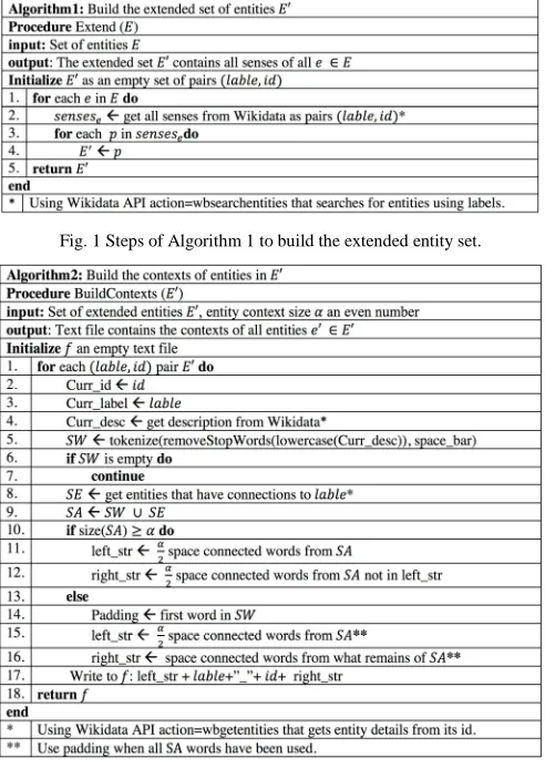
thirteen_colonies_q179997. The words “federal” and “republic” are elements of SW whereas the entities “new_york_city_q60” and “thirteen_colonies_q179997” are elements of SE .Algorithms 1 and 2 shown in Fig. 1 and Fig. 2 respectively explain the functionalities of the crawler in detail.
Fig. 1 Steps of Algorithm 1 to build the extended entity set.
Fig. 2 Steps of Algorithm 2 to build the contexts of target entities.
B. Building Joint Vector Representations
To build the joint vector representations of words and entities in the same vector space, we extend the CBOW model proposed in [1] to cover not only words but also entities as well. We will use the result of the crawler as the training input. Each line in the output text file contains the context of a specifically named entity sense. Pairs of training examples w , w' are generated only within the same line to predict the target entity w' from a context elementw . Therefore, the training is achieved by maximizing the following objective function using stochastic gradient descent (SGD):
1
( ) ) Log - .′/|123 4
567 8
/67
(1)
where L is the total number of entities in the extended entity set 9′, .′/ is an entity in 9′, α is the entity context size and
123 ∈ : .′/ is a co-word or a co-entity from the .′/ context. To avoid complexity, we use NEG proposed in [17], defined by the following objective function:
Log - ./|123 = Log σ <=>
? < @A5
+ ) BCD~FGC HLog σ −<CD ? <
@A5 I J
K67
(2)
Where σ x = 7
7M N ON is the sigmoid function, P is the number of negative samples (noise words) indicated as QK and taken from the noise distribution -R Q defined as:
-R Q = S Q T U
∑ SWQ5X T U R
56Y
(3)
Where f is the frequency of the word Q in a vocabulary of size n.
We maximize the objective function in equation (1) using a two-layer neural network similar to the structure of the word2vect model [17]. The vector representations (embedding) of the words and entities will be stored as the rows of the weight matrix of the model’s hidden layer. To maintain vectors properties in the Euclidean space for the following steps, embedding are normalized using ℓ$ norm as per equation (4):
]R^_` = ]
a∑ |]bK67 K|$ (4)
where ] is an embedding vector of length c.
C. Building the Final Entity Vector Representations
After building the joint vector representations by training to predict the target entity .′ from its context’s words and entities, the final entity representations are built using the embedding of prominent elements from the corresponding contexts. To remove redundant features and emphasize the distinctive ones, entity representations are compressed into high level compact vector representations using auto encoders. The concept of auto encoders were first discussed in [14] and then used in [25] as unsupervised neural networks trained to produce their inputs as outputs. Auto encoders composed of two parts: the encoder .de ] and the decoder f.e ] . Both can be seen as neural networks with multiple hidden layers. The encoder maps its input vector
op3 = ) ||<K− f.e .de <K ||$ 8
K67
(5)
After training the auto encoder, the vectors produced by the encoder part can be seen as compact representations of the input vectors. These representations contain knowledge good enough to rebuild the original vectors with high confidence. The encoder part can be used to map the training vectors of S to a new vector space with smaller dimension and use the new set of vectors to train another autoencoder. This structure is called a stacked auto encoders, which represents a deep neural network with many hidden layers.
We use a two-layer stacked under complete auto encoders to build the final entity representations. This allows for capturing high-level abstract features about the entities. Each auto encoder consists of two hidden layers in the encoding part and two hidden layers in the decoding part. The first auto encoder is trained using input vectors that represent the target entity contexts. These vectors are built by concatenating the embedding of β chosen context elements, which can be either a co-word, a co-entity or the target entity itself. The context elements are chosen in a way to keep the most distinctive features about the context. These elements are then ordered alphabetically, and their embedding is concatenated to construct the first auto encoder training vectors. We chose β − 1 elements that have the highest average distances from the embeddings of the remaining context elements. These elements are the top β − 1 elements from the context that maximize the objective function in equation 6. To include features from the rest of the context, the element with the smallest average distance from all the other context elements, i.e. the element that minimizes the objective function in equation 6 is also chosen. We call this element the context agent. This way, the chosen context elements maximize the chances of keeping the most descriptive features about the target entities.
r s =t ) f1 4M7
K67.FD vw
-K, s (6)
Where s, -K are embeddings of context elements in the vector space ℝx where z is the embedding vector size, α is the context size and f -K, s is the Euclidean distance between Pi and Q.
Each auto encoder has two hidden layers, and each hidden layer is half the size of the previous layer. This gives the used stacked auto encoders structure a vector-compressing factor of 16. The size of the input vectors of the first auto encoder is z × β. We train the first auto encoder to represent the size x×{U which is the size of the input vectors to be used to train the second auto encoder. The final entity embedding
has a size of x×{
7| moreover; it is obtained from the encoder part of the second auto encoder.
In our experiments, we use Wikidata as the source of the training set of named entities. We collected top 500 named entities from Wikidata using a simple collection algorithm that automatically checks Wikidata entities starting from
id = 1 and an empty set E. The algorithm heuristically checks the label in the corresponding Wikidata page looking for named entities. Detected entities will be added to the entity set E. Crawler Algorithm 1 in Fig. 1 is then used to
build the extended entity set E′ with all entity senses. The size of the built set E′ is 1559 with an average of about three senses per entity. The extended set is then used as input to crawler’s Algorithm 2 in Fig. 2 to build the contexts C e For all e′ ∈ E′ with a fixed context size α = 14. The output is a text file contains 1559 lines representing entity contexts. For example, the named entity “Syria” in the set E has 6 senses in E′ where it can be either a country, female name, journal name, a Roman province, Italian singer or a family name. Related co-words and co-entities surround each of these six senses. For example, the country sense is written as Syria_q858 with neighbors such as Asia, republic, damascus_q3766, turkey_q43, etc. The singer sense is written as Syria_q3979196 with neighbors including Italian, singer, italy_q38, and rome_q220.
The second step is to train the model described in section III.B using the crawler’s output text file. We use Google’s Tensor flow Python library [26] to implement the two-layer neural network where the input and output layers have the same size as the vocabulary size. The vocabulary size is the number of unique words/entities in the input text file. The hidden layer’s size equals the required embedding vectors size. We set the embedding size, i.e. the size of the hidden layer to 128. We set the rest of the model’s parameters like the following: the number of negative samplesNEG = 64, gradient descent learning rate is set to 1.0. Training examples are generated from each line as pairs w , w' where w'the target entity of the line is and wis a context element. Since we use a context size of 14, each line can produce 14 training pairs. The model is trained for 100,000 iterations using a batch of training pairs. We use a batch size of 280 to cover all pairs of 20 randomly selected contexts in the same training batch. Once the model training is completed, the hidden layer’s weight matrix is saved as the embedding of the training vocabulary. It contains the embedding of both words and entities mapped to the same vector space.
To build the final entity representations, we train the stacked auto encoders model to minimize the construction error of L = 1559 vectors in the input set S as per equation 5. We choose β = 4, and thus the size of each training vector is
128 × 4 = 512 which is the size of the input layer of the first autoencoder. The first autoencoder is trained for 30,000 iterations with a learning rate of 0.05 using batches of size 256. It is trained to encode the input to a vector of size 128 which is the size of the input layer of the second auto encoder. The second auto encoder is then trained using similar parameters except with a learning rate of 0.01. After training the second auto encoder, the two stacked auto encoders model is now ready to be used to encode input vectors. The result is a set of L vectors of size 32 that includes the final vector representations of the target named entities.
III.RESULTS AND DISCUSSION
As described in section III.C, the β context elements that will be used to build the final entity representations can be either words or entities. Denoting the chosen set for an entity
statistical analysis of the distribution of β elements considering all the 1559 test entities and their contexts.
TABLE I
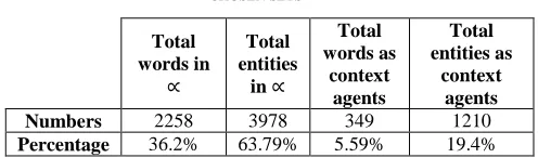
STATISTICAL ANALYSIS OF THE DISTRIBUTION OF Š ELEMENTS OF ALL CHOSEN SETS Total words in ∝ Total entities
in ∝
Total words as context agents Total entities as context agents
Numbers 2258 3978 349 1210
Percentage 36.2% 63.79% 5.59% 19.4%
As TABLE I shows, entities are chosen at almost twice the rate of choosing words to be in the β chosen elements of target entities. This is largely because the number of co-words in any context is less than the number of co-entities. The only source of the co-words is the Wikidata description text which is usually not more than a couple of sentences. However, Wikidata page of an entity has plenty of co-entities found in the binary relations of the target entity.
To evaluate the final vector representations of entities, we use cosine similarity as a measure of the semantic similarity between two vectors in the space. We find the closest entity to all the 1559 test entities by finding the entity from the same set with the maximum cosine similarity. Since an entity with a maximum cosine similarity can always be found, a threshold has to be set to consider that the entities are semantically related. This threshold depends on the size and coverage of the training entity set. For small domain-specific training sets, this threshold has to be large and very close to 1. TABLE II shows some examples of the most similar entities found in the used training set with cosine similarities more than 0.95.
TABLE II
SOME EXAMPLES OF SIMILAR ENTITIES IN THE USED TRAINING SET WITH COSINE SIMILARITIES MORE THAN 0.95.
Related entities Wikidata descriptions Bolivia_Q750
& Paraguay_Q733
A country in South America &
A country in South America Moscow_Q2380475
& Lisbon_Q2310637
City in Tennessee, USA &
A town in New Hampshire, USA Maine_Q3708887
& Flanders_Q3459889
A town in New York, United States &
Census-designated place in Suffolk County, New York Versailles_Q2729504
& Rhine_Q1886951
A town in Indiana, United States &
A civil town in Sheboygan County, Wisconsin
Egypt_Q2083973 & Versailles_Q2729504
Town in Arkansas &
A town in Indiana, United States Lebanon_Q1520670
& London_Q3061911
City in Wilson County &
Tennessee, a city in Kentucky, United States
Panama_Q2204538 & Lisbon_Q2384470
Town in Oklahoma &
A town in Maine, USA
August_Q1192731 &
We_Live_In_Public_Q372
2008 American drama film &
2009 documentary film by Ondi Timoner which profiles internet
pioneer Josh Harris Sunday_Q1286562
& Dubai_Q5310496
Song by British recording duo Hurts &
2005 Filipino drama film
As TABLE II shows, the cosine similarity is close to 1 for entities that represent the same real-world concepts such as cities, countries, and films. Entities that are semantically related such as city, town, and community also have high cosine similarities i.e. more than 0.95. The last row in TABLE II is another example of how semantically related entities are assigned similar representations where both entities represent the artwork concept.
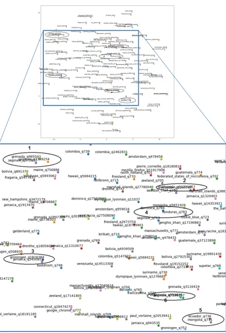
To show how entities of our training set are distributed in the vector space, we use the non-linear dimensionality reduction tool t-SNE [27] to visualize entity embeddings in the 2D space. Fig. 3 shows the distribution of 150 randomly chosen entity embeddings.
As expected, Fig. Three shows that semantically related entities are clustered relatively near each other in the vector space. TABLE III shows a few examples of related entities found in Fig. 3 where examples are numbered from 1 to 6.
TABLE III
EXAMPLES OF RELATED ENTITIES FOUND IN FIG. 3
Group
# Related entities Wikidata descriptions
1 Grenada_Q985543 & Saginaw_Q7399254 & Saginaw_Q970802
City in Mississippi & An unincorporated community in Hot Spring
County, Arkansas & City in Texas
2 Guatemala_Q11221957 & Ecuador_Q2347797 Triceratops song & 1997 song by Sash!
3
Groningen_Q1816384 & Jamaica_Q3450853
An unincorporated community in Pine County,
Minnesota &
A town in Vermont, United States
4
Dominica_Q784 & Honduras_Q783
A country in the Caribbean &
Republic in Central America
5
Ecuador_Q736 & Mongolia_Q711
A country in South America &
A country in East Asia, between China and Russia
6
Venezuela_Q593830 & Saginaw_Q7399257
City in Cuba & An unincorporated community in St. Louis
Fig. 3 also shows that not all close entities are semantically related. As discussed earlier, a high similarity threshold is required for small training sets. This translates to a short distance between related vectors especially after reducing the dimension of embedding for visualization using t-SNE.
The goal of constructing entity embedding for ontology population tasks requires that if two entities share similar contexts, then their embedding are expected to be similar and vice versa. To test this using our training set, we find all unique entity pairs where the cosine similarity is more than 0.95. Then we check the corresponding contexts looking for shared elements, i.e. shared co-words or co-entities. We consider the pair as correct if there is at least one shared element found in their contexts, which justifies the high similarity. For example, the entities Bolivia_Q750 and Paraguay_Q733 have a cosine similarity of more than 0.95. For this pair to be considered as correct which means that they were rightfully assigned similar representations, they should have common elements in their contexts. By checking their contexts, we find that four elements are shared: Spanish_Q1321, South_america_Q18, south, and country. The first two are named entities, and last two are words. Based on this, the pair is considered as correct.
Out of 963 unique pairs found, 951 pairs share context elements with an accuracy of 98.75%. This means that entities with similar contexts have a high change of being assigned close embedding. It is also worth noting that the remaining pairs are not necessarily false positives since we look for the exact elements in both contexts. Contexts may share synonyms or other semantically related elements that caused the embedding to be similar which is the expected behavior of good embedding. We repeated the experiment using different thresholds to test the effect on the accuracy. Table I shows the accuracies for different similarity thresholds.
TABLE IV
ACCURACIES FOR DIFFERENT SIMILARITY THRESHOLDS
Similarity threshold
Unique entity pairs
with similarity >
threshold
Pairs with at least one shared context element
Accuracy
0.95 963 951 98.75%
0.93 1636 1578 96.34%
0.90 3199 2783 86.99%
0.85 11050 6535 59.14%
As Table II shows, the number of unique entity pairs increases when using lower thresholds with a large number of wrong entity pairs. This is mainly due to the small size of the training set. Covering a large amount of entities increases the chances of the relatedness between close entities. Using a larger set helps to discover new correct pairs of similar entities and keeps the number of false positives very low when using low thresholds.
IV.CONCLUSIONS
In this paper, we presented a method to build entity vector representations using knowledge from Wikidata. These representations hold distinctive features about the entities,
which help to identify the correct entity sense in natural language text to facilitate ontology population tasks. Ontology population, which is the process of adding new instances of concepts and relations into an ontology from a corpus, will benefit from this process in order to minimize the manual effort as exhibited in [28].
The conducted experiments show that entities are assigned close vector representations if they have similar contexts. In the future, we plan to demonstrate the use of the constructed entity vectors in the tasks NED and relation extraction. It would also be interesting to investigate the effect of using Wikidata hierarchies while building entity contexts.
REFERENCES
[1] T. Mikolov, K. Chen, G. Corrado, and J. Dean, “Efficient estimation of word representations in vector space,” arXiv preprint arXiv:1301.3781, 2013.
[2] M. A. Taiye, S. S. Kamaruddin, and F. K. Ahmad, “Representing Semantics of Text by Acquiring its Canonical Form,” International Journal on Advanced Science, Engineering and Information Technology, vol. 7, no. 3, pp. 808-814, 2017.
[3] S. A. M. Noah, N. Omar, and A. Y. Amruddin, “Evaluation of lexical-based approaches to the semantic similarity of Malay sentences.,” Journal of Quantitative Linguistics, vol. 22, no. 2, pp. 135-156, 2015.
[4] M. Mohd and O. M. A. Bashaddadh, “Investigating the Combination of Bag of Words and Named Entities Approach in Tracking and Detection Tasks among Journalists.,” Journal of Information Science Theory and Practice, vol. 2, no. 4, pp. 31-48, 2014.
[5] N. I. Y. Saat and S. A. M. Noah, “Rule-based Approach for Automatic Ontology Population of Agriculture Domain,” Information Technology Journal, vol. 46, no. 51, pp. 46-51, 2016. [6] Y. I. A. M. Khalid and S. A. M. Noah, “Semantic text-based image
retrieval with multi-modality ontology and DBpedia,” The Electronic Library, vol. 35, no. 6, pp. 1191-1214, 2017.
[7] W. Ammar, G. Mulcaire, Y. Tsvetkov, G. Lample, C. Dyer and N. A. Smith, “Massively Multilingual Word Embeddings,” arXiv preprint arXiv:1602.01925, 2016.
[8] R. E. Salah and L. Q. b. Zakaria, “Arabic Rule-Based Named Entity Recognition Systems: Progress and Challenges,” International Journal on Advanced Science, Engineering and Information Technology, vol. 7, no. 3, pp. 815-821, 2017.
[9] Z. S. Harris, “Distributional structure,” Word, vol. 10, no. 2-3, pp. 146 - 162, 1954.
[10] J. R. Firth, “A synopsis of linguistic theory 1930-55,” in Studies in Linguistic Analysis, Vols. 1952-59, The Philological Society, 1957, pp. 1-32.
[11] M. Sahlgren, “The distributional hypothesis,” Italian Journal of Disability Studies, vol. 20, pp. 33-53, 2008.
[12] G. Salton, The SMART Retrieval System—Experiments in Automatic Document Processing, NJ: Prentice-Hall, Inc. Upper Saddle River, 1971.
[13] D. E. Rumelhart and J. L. McClelland, Psychological and Biological Models, MIT Press, 1986.
[14] D. E. Rumelhart, G. E. Hinton, and R. J. Williams, “Learning internal representations by error propagation,” in Parallel distributed processing: explorations in the microstructure of cognition, Cambridge, MA, MIT Press Cambridge, MA, 1986.
[15] Y. Bengio, R. Ducharme, P. Vincent, and C. Jauvin, “A Neural Probabilistic Language Model,” Journal of Machine Learning Research, vol. 3, pp. 1137-1155, 2003.
[16] T. Mikolov, W.-t. Yih, and G. Zweig, “Linguistic regularities in continuous space word representations,” in Proceedings of the 2013 Conference of the North American Chapter of the Association for Computational Linguistics: Human Language Technologies, 2013. [17] T. Mikolov, I. Sutskever, K. Chen, G. Corrado, and J. Dean,
[18] M. U. Gutmann and A. Hyvärinen, “Noise-contrastive estimation of unnormalized statistical models, with applications to natural image statistics,” The Journal of Machine Learning Research, vol. 13, no. 1, pp. 307-361, 2012.
[19] I. Yamada, H. Shindo, H. Takeda, and Y. Takefuji, “Joint learning of the embedding of words and entities for named entity disambiguation,” arXiv preprint arXiv:1601.01343, 2016.
[20] D. Milne and I. H. Witten, “An effective, low-cost measure of semantic relatedness obtained from Wikipedia links,” in In Proceedings of the First AAAI Workshop on Wikipedia and Artificial Intelligence (WIKIAI), 2008.
[21] Z. Wang, J. Zhang, J. Feng, and Z. Chen, “Knowledge graph and text jointly embedding,” in Proceedings of the 2014 conference on empirical methods in natural language processing (EMNLP), 2014. [22] Y. Cao, L. Huang, H. Ji, X. Chen and J. Li, “Bridging Text and
Knowledge by Learning Multi-Prototype Entity Mention Embedding,” in Proceedings of the 55th Annual Meeting of the Association for Computational Linguistics (Volume 1: Long Papers), 2017. [23] J. G. Moreno, R. Besancon, R. Beaumont, E. D'hondt, A.-L. Ligozat,
S. Rosset, X. Tannier and B. Grau, “Combining word and entity
embeddings for entity linking,” in European Semantic Web Conference, 2017.
[24] Freebase, 17 December 2014. [Online]. Available: https://plus.google.com/109936836907132434202/posts/bu3z2wVqc Qc.
[25] D. H. Ballard, “Modular learning in neural networks,” in AAAI'87 Proceedings of the sixth National conference on Artificial intelligence, 1987.
[26] M. Abadi, A. Agarwal, P. Barham, E. Brevdo, Z. Chen, C. Citro, G. S. Corrado, A. Davis, J. Dean, M. Devin, S. Ghemawat, I. Goodfellow, A. Harp, G. Irving, M. Isard, Y. Jia, R. Jozefowicz and L, “Tensorflow: Large-scale machine learning on heterogeneous distributed systems,” arXiv preprint arXiv:1603.04467, 2016. [27] L. v. d. Maaten and G. Hinton, “Visualizing data using t-SNE,”
Journal of machine learning research, pp. 2579-2605, 2008. [28] Z. Ibrahim, S. A. M. Noah and M. M. Noor, “Knowledge acquisition