www.geosci-model-dev.net/9/4365/2016/ doi:10.5194/gmd-9-4365-2016
© Author(s) 2016. CC Attribution 3.0 License.
A diagram for evaluating multiple aspects of model performance in
simulating vector fields
Zhongfeng Xu1, Zhaolu Hou2,3,4, Ying Han1, and Weidong Guo2,5
1RCE-TEA, Institute of Atmospheric Physics, Chinese Academy of Sciences, Beijing, China
2Institute for Climate and Global Change Research, School of Atmospheric Sciences, Nanjing University, Nanjing, China 3LASG, Institute of Atmospheric Physics, Chinese Academy of Sciences, Beijing, China
4University of Chinese Academy of Sciences, Beijing, China
5Joint International Research Laboratory of Atmospheric and Earth System Sciences, Nanjing, China
Correspondence to:Zhongfeng Xu ([email protected])
Received: 3 July 2016 – Published in Geosci. Model Dev. Discuss.: 1 August 2016 Revised: 28 October 2016 – Accepted: 7 November 2016 – Published: 6 December 2016
Abstract. Vector quantities, e.g., vector winds, play an ex-tremely important role in climate systems. The energy and water exchanges between different regions are strongly dom-inated by wind, which in turn shapes the regional climate. Thus, how well climate models can simulate vector fields directly affects model performance in reproducing the na-ture of a regional climate. This paper devises a new diagram, termed the vector field evaluation (VFE) diagram, which is a generalized Taylor diagram and able to provide a concise evaluation of model performance in simulating vector fields. The diagram can measure how well two vector fields match each other in terms of three statistical variables, i.e., the vec-tor similarity coefficient, root mean square length (RMSL), and root mean square vector difference (RMSVD). Similar to the Taylor diagram, the VFE diagram is especially useful for evaluating climate models. The pattern similarity of two vector fields is measured by a vector similarity coefficient (VSC) that is defined by the arithmetic mean of the inner product of normalized vector pairs. Examples are provided, showing that VSC can identify how close one vector field re-sembles another. Note that VSC can only describe the pattern similarity, and it does not reflect the systematic difference in the mean vector length between two vector fields. To mea-sure the vector length, RMSL is included in the diagram. The third variable, RMSVD, is used to identify the magnitude of the overall difference between two vector fields. Examples show that the VFE diagram can clearly illustrate the extent to which the overall RMSVD is attributed to the systematic difference in RMSL and how much is due to the poor pattern similarity.
1 Introduction
Vector quantities play a very important role in climate sys-tems. It is well known that atmospheric circulation transfers mass, energy, and water vapor between different parts of the world, which is an extremely crucial factor for shaping re-gional climates. The monsoon climate is a typical example of one that is strongly dominated by atmospheric circula-tion. A strong Asian summer monsoon circulation usually brings more precipitation, and vice versa. Therefore, the sim-ulated precipitation is strongly determined by how well cli-mate models can simulate atmospheric circulation (Twardosz et al., 2011; Sperber et al., 2013; Zhou et al., 2016; Wei et al., 2016). Ocean surface wind stress is another important vector quantity that reflects the momentum flux between the ocean and atmosphere, serving as one of the major factors for oceanic circulation (Lee et al., 2012). The wind stress errors can cause large uncertainties in ocean circulation in the sub-tropical and subpolar regions (Chaudhuri et al., 2013). Thus, the evaluation of vector fields, e.g., vector winds and wind stress, would also help in understanding the causes of model errors.
and centered root mean square error (RMSE), do not ap-ply to vector quantities. No such diagram is yet available for evaluating vector quantities such as vector winds, wind stress, temperature gradients, and vorticity. Previous studies have usually assessed model performance in reproducing a vector field by evaluating its x andy components with the Taylor diagram (e.g., Martin et al., 2011; Chaudhuri et al., 2013). Although such an evaluation can also help to exam-ine the modeled vector field, it suffers from some deficien-cies. (1) A good correlation in the x andy components of the vector between the model and observation may not nec-essarily indicate that the modeled vector field resembles the observed one. For example, assuming we have two identical two-dimensional vector fieldsAandBtheir correlation coef-ficients are 1 for both thexandycomponents. If thex com-ponent of vector fieldAadds a constant value, the correlation coefficients for both thex andy components do not change, but the direction and length of vectorAchange, which sug-gests that the pattern of two vector fields are no longer identi-cal. Thus, computing the correlation coefficients for thexand y components of a vector field is not well suited for examin-ing the pattern similarity of two vector fields. (2) It is hard to determine the improvement of model performance. For ex-ample, should one conclude that the model performance is improved if the RMSE (or correlation coefficient) is reduced for theycomponent but increased for thex component of a vector field? Given these reasons and the importance of vec-tor quantities in a climate system, we have developed a new diagram, termed the vector field evaluation (VFE) diagram, to measure multiple aspects of model performance in simu-lating vector fields.
To construct the VFE diagram, one crucial issue is quan-tifying the pattern similarity of two vector fields. Over the past several decades, many vector correlation coefficients have been developed by different approaches. For example, some vector correlation coefficients are constructed by com-bining Pearson’s correlation coefficient of thex andy com-ponents of the vector (Charles, 1959; Lamberth, 1966). Some vector correlation coefficients are devised based on orthogo-nal decomposition (Stephens, 1979; Jupp and Mardia, 1980; Crosby et al., 1993) or the regression relationship of two vec-tor fields (Ellison, 1954; Kundu, 1976; Hanson et al., 1992). These vector correlation coefficients usually do not change when one vector field is uniformly rotated or reflected to a certain angle. This is a reasonable and necessary property for the vector correlation coefficient when one detects the re-lationship of two vector fields. However, in terms of model evaluation, we expect the simulated vectors to resemble the observed ones in both direction and length with no rotation permitted. Thus, previous vector correlation coefficients are not well suited for the purpose of climate model intercom-parisons and evaluation.
To measure how well the patterns of two vector fields re-semble each other, a vector similarity coefficient (VSC) is introduced in Sect. 2 and interpreted in Sect. 3. Section 4
constructs the VFE diagram with three statistical variables to evaluate multiple aspects of simulated vector fields. Sec-tion 5 illustrates the use of the diagram in evaluating cli-mate model performance. Methods for indicating observa-tional uncertainty are suggested in Sect. 6. A discussion and conclusion are provided in Sect. 7.
2 Definition of vector similarity coefficient
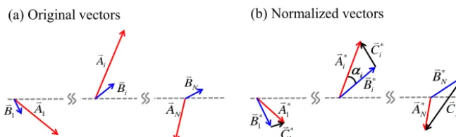
Consider two vector fieldsAandB (Fig. 1a). Without loss of generality, vector fieldsAandB can be written as a pair of vector sequences.
Ai=(xai, yai); i=1,2, . . ., N Bi =(xbi, ybi); i=1,2, . . ., N
Each vector sequence is composed ofN vectors. To mea-sure the similarity between vector fieldsAandB, a vector similarity coefficient (VSC) should be able to recognize to what degree the vectors are in the same direction and how much the vector lengths are proportional to each other. Thus, VSC is defined as follows:
Rv= N
P
i=1 Ai•Bi
s
N
P
i=1
|Ai|2
s
N
P
i=1
|Bi|2
, (1)
where||represents the length of a vector. The•symbol rep-resents the inner product.
We define a normalized vector as follows:
A∗i = Ai s
1 N
N
P
i=1
|Ai|2
= Ai LA
(2)
and
B∗i = Bi s
1 N
N
P
i=1
|Bi|2
= Bi LB
, (3)
respectively, where
LA=
v u u t 1 N
N
X
i=1
|Ai|2 (4)
and
LB=
v u u t 1 N
N
X
i=1
|Bi|2 (5)
(a) Original vectors (b) Normalized vectors
Figure 1.Schematic illustration of two vector sequences. Panel(a)original vectors and(b)normalized vectors. The length of vector se-quenceAi is systematically greater than that of vector sequenceBi. The normalization only alters the lengths of vectors without changes in directions.
and variance of vector lengths (Eq. A1). Based on Eqs. (2) and (3), we have
N
X
i=1
A ∗ i 2 = N X
i=1
B ∗ i 2
=N. (6)
Clearly, the normalization of a vector field only scales the vector lengths without changing their directions (Fig. 1b).
With the aid of Eqs. (2) and (3), Eq. (1) can be rewritten as
Rv=
1 N
N
X
i=1
A∗i •B∗i
= 1 N
N
X
i=1
A ∗ i B ∗ i cosαi
= 1 N
N
X
i=1
A∗i
2
+B∗i
2
−C∗i
2
2 =1− 1
2N
N
X
i=1
C∗i
2
=1−1
2MSDNV
, (7)
whereC∗i is the difference between the normalizedAandB
(Fig. 1b). MSDNV is the mean square difference of the nor-malized vectors (Shukla and Saha, 1974, with minor modifi-cation) between two normalized vector sequences:
MSDNV=1 N
N
X
i=1
A∗i −B∗i 2 = 1 N N X
i=1
C∗i
2
. (8)
Given the triangle inequality, 0≤C∗i ≤
A∗i
+
B∗i
, we have
0≤C ∗ i
2
≤ A ∗ i + B ∗ i 2≤ 2A
∗ i
2
+2B ∗ i 2 . (9) With the aid of Eqs. (6), (7), (8), and (9), we obtain
0≤MSDNV≤4, and−1≤Rv≤1.
Rv reaches its maximum value of 1 when MSDNV=0,
i.e.,A∗i =B∗i for alli(1≤i≤N).Rvreaches its minimum
value of −1 when MSDNV=4, i.e., A∗i = −B∗i for all i (1≤i≤N). Thus, the vector similarity coefficient,Rv,
al-ways takes values in the intervals [−1, 1] and is determined by MSDNV, namelyN1
N
P
i=1
C∗i
2
. Clearly,C∗i
is determined by the differences in both vector lengths and angles between
A∗i and B∗i (Fig. 1b). A smaller C∗i
suggests that A∗i is closer toB∗i, and vice versa. To better understandRv, some
special cases are discussed as follows. For alli(1≤i≤N):
– If A∗i =B∗i, then C∗i
=0. We obtain Rv=1 when
each pair of normalized vectors is exactly the same length and direction.
– IfA∗i = −B∗i, thenA∗i =
B∗i
=
C∗i
/2. We obtain Rv= −1 when each pair of normalized vectors is
ex-actly the same length but goes in opposite directions. – If A∗i ⊥B∗i, then A∗i
2
+B∗i
2
=C∗i
2
. We obtain Rv=0 when each pair of normalized vectors is
orthog-onal to each other. – IfC∗i
2
<A∗i
2
+B∗i
2
, we obtain 0< Rv<1 when
the angles betweenA∗i andB∗i are acute angles. – IfC∗i
2
>A∗i
2
+B∗i
2
, we obtain−1< Rv<0 when
the angles betweenA∗i andB∗i are obtuse angles. Thus, a positive (negative)Rvindicates that the angles
be-tweenA∗i andB∗
i are generally smaller (larger) than 90 ◦, which suggests that the patterns betweenA∗i andB∗
i are
sim-ilar (opposite) to each other. A greaterRvindicates a higher
similarity between two vector fields. Based on Eqs. (2), (3), and (7),Rvdoes not change whenAorB is multiplied by
a positive constant, which is analogous to the property of Pearson’s correlation coefficient. Thus,Rv can measure the
3 Interpreting VSC
In this section, we present three cases to explain why VSC can reasonably measure the pattern similarity of two vector fields. To facilitate the interpretation, we define the mean dif-ference of angles (MDA) between paired vectors as follows: MDA= ¯α= 1
N
N
X
i=1
αi=
1 N
N
X
i=1
acos A
i•Bi
|Ai||Bi|
, (10) where the vector fields Aand B are the same as those in the Eq. (1).αi is the included angle between paired vectors.
MDA takes values in intervals [0,π] and measures how close the corresponding vector directions of two vector fields are to each other. A mean square difference (MSD) of normalized vector lengths is defined as follows:
MSD=1 N
N
X
i=1
A ∗ i − B ∗ i 2 = 1 N N X
i=1
A∗i
2
+B∗i
2
−2A∗i B∗i
=2− 2 N
N
X
i=1
A ∗ i B ∗ i . (11)
Given Eq. (6) and the Cauchy–Schwarz inequality,
N
X
i=1
A ∗ i B ∗ i !2 ≤ N X
i=1
A ∗ i
2XN
i=1
B ∗ i 2 ,
we find that MSD takes on values in intervals [0, 2]. For alli(1≤i≤N), ifA∗i
=
B∗i
, we have MSD=0. For alli(1≤i≤N), ifA∗i
B∗i
=0, we have MSD=2. MSD measures how close the paired vector lengths of two normalized vector fields are to each other. Based on the def-inition ofRv(Eq. 7), the VSC is determined by both
differ-ences in vector lengths and angles between two groups of vectors. To interpret the nature of VSC, we will discuss how VSC will change with MSD and MDA in Sect. 3.1 and 3.2, respectively.
3.1 Interpreting VSC based on its equation VSC can be written as follows:
Rv=
1 N
N
X
i=1
A∗i •B∗i
= 1 N
N
X
i=1
A∗i
B∗i
cosαi = 1 N N X
i=1
A∗i
2
+B∗i
2 − A∗i
−
B∗i
2
2
cosαi
.
To examine the relationship of VSC with MSD, we assume each corresponding angle between paired vectorsαi=α=
const (i= [1, N]). With the support of Eqs. (6) and (11), we obtain
Rv=
" 1− 1
2N
N
X
i=1
A∗i
−
B∗i
2 # cosα =
1−MSD 2
cosα
. (12)
Thus,Rvvaries between 0 and cosαdue to the difference
in the normalized vector length whenαis a constant angle. Rv equals 0 when α equals 90◦ regardless of the value of
MSD. MSD plays an increasingly important role in determin-ingRvwhenαapproaches 0 or 180◦.Rvis inversely
propor-tional to MSD, which suggests that two vector fields show a higher similarity when their corresponding normalized vec-tor lengths are closer to each other, and vice versa. On the other hand,Rv is proportional to cosα, suggesting a higher
VSC when the directions of paired vectors are closer to each other. This indicates that VSC can reasonably describe how close the normalized vector fields are by taking both vec-tor lengths and directions into consideration simultaneously (Eq. 12).
3.2 Interpreting VSC based on random generated samples
In the previous section, the interpretation of VSC is based on the assumption that the paired vectors have a constant in-cluded angle. In this section, we will examine how VSC is affected by the difference of included angles in a more gen-eral case. Firstly, we construct a reference vector sequence,
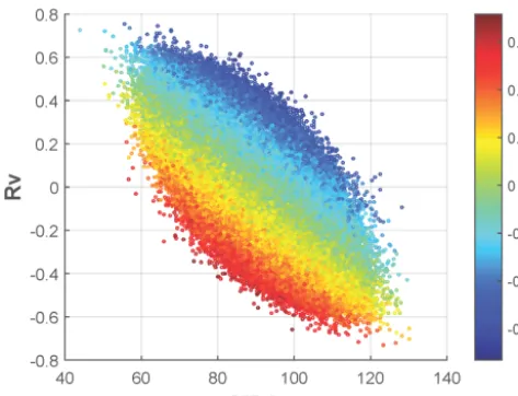
A, comprising 30 vectors, i.e.,i= [1,30]. The lengths of 30 vectors follow a normal distribution, and the arguments of 30 vectors follow a uniform distribution between 0 and 360◦. Secondly, we produced a new vector sequenceBby rotating each individual vector ofAby a certain angle randomly be-tween 0 and 180◦ without changes in vector lengths. Such a random generation of B was repeated 1×10⁶ times to produce sufficient random samples of vector sequences. The vector similarity coefficientRvis computed betweenAand
the 1×10⁶sets of randomly produced vector sequences, re-spectively. As shown in Fig. 2,Rvgenerally shows a negative
relationship with MDA, i.e., a smaller MDA generally corre-sponds to a largerRv, and vice versa. A smaller MDA
in-dicates smaller differences in the directions of paired vectors and hence a higher similarity between the vector fieldsAand
B, suggesting that VSC can reasonably describe how close the vector directions between two vector fields are. Mean-while, it is also noted thatRvvaries within a large range for
the same MDA. For example, when MDA equals 90◦,R v
can vary from approximately−0.5 to 0.5 depending on the relationship between the paired vector lengths and the corre-sponding included angles (Fig. 2). A positive (negative)Rvis
Figure 2.Scatterplot between the vector similarity coefficient (Rv) and mean difference of angle (MDA) derived from the reference vector field A and randomly generated vector fieldB. There are 106random vector fieldsB included in the statistics. The colors denote the correlation coefficients between the vector length and the included angle between two vector sequences.
(large). Specifically, the rotation of shorter vectors may not undermineRvtoo much as long as the longer vectors remain
unchanged. In contrast, Rv would be strongly undermined
with the rotation of longer vectors. Simply put, the longer vectors generally play a more important role than the shorter vectors in determiningRv.
3.3 Application of VSC to 850 hPa vector winds In this section, we compute theRvof the climatological mean
850 hPa vector winds in January with that in each month in the Asian–Australian monsoon region (10◦S–40◦N, 40– 140◦E). The purpose of this analysis is to further illustrate whether or notRvcan measure the similarity of two vector
fields with observational data. The wind data used are NCEP-DOE Reanalysis 2 data (Kanamitsu et al., 2002). The cli-matological mean 850 hPa vector winds show a clear winter monsoon circulation characterized by northerly winds over the tropical and subtropical Asian regions in January and February (Fig. 3a, b). The spatial pattern of vector winds in January is very close to that in February, which corresponds to a very highRv(0.97). The spatial pattern of vector winds
in January is less similar to that in April and October, which corresponds to a weakRvof 0.48 and−0.11, respectively. In
August, the spatial pattern of 850 hPa winds is generally op-posite of that in January, which corresponds to a negativeRv
(−0.64). The VSCs of 850 hPa vector winds between clima-tological January and each climaclima-tological month show a clear annual cycle characterized by a positiveRvin the cold
sea-son (November–April) and a negativeRvin the warm season
(June–September) in the Asian–Australian monsoon region
(Fig. 3f, solid line). Figure 3 illustrates that VSC can rea-sonably measure the pattern similarity of two vector fields. We also computed the VSCs of 850 hPa vector winds be-tween climatological January and each individual month dur-ing the period from 1979 to 2005, respectively. The VSCs show a smaller spread in winter (January, February, and De-cember) and summer (June, July, and August) months than during the transitional months such as April, May, and Octo-ber (Fig. 3f). This indicates that the spatial patterns of vector winds have smaller interannual variation in summer and win-ter monsoon seasons than during the transitional seasons.
4 Construction of the VFE diagram
To measure the differences in two vector fields, a root mean square vector difference (RMSVD) is defined follow-ing Shukla and Saha (1974) with a minor modification:
RMSVD= "
1 N
N
X
i=1
|Ai−Bi|2 #12
,
whereAi andBi are the original vectors. The RMSVD
ap-proaches zero when two vector fields become more alike in both vector length and direction. The square of RMSVD can be written as
RMSVD2= 1 N
N
X
i=1
|Ai−Bi|2
= 1 N
N
X
i=1
|Ai|2+ |Bi|2−2|Ai•Bi|
= 1 N
N
X
i=1
|Ai|2+
1 N
N
X
i=1
|Bi|2−
2 NRv
• s
N
P
i=1
|Ai|2 N
P
i=1
|Bi|2
= 1 N
N
X
i=1
|Ai|2+
1 N
N
X
i=1
|Bi|2−2Rv
• v u u t 1 N
N
X
i=1
|Ai|2
v u u t 1 N
N
X
i=1
|Bi|2
.
With the support of Eqs. (4), (5), and (7), we obtain
RMSVD2=L2A+L2B−2Rv•LALB. (13)
The geometric relationship between RMSVD, LA, LB,
and Rv is shown in Fig. 4, which is analogous to Fig. 1
in Taylor (2001) but constructed by different quantities. It should be noted that RMSVD is computed from the two orig-inal sets of vectors. However, the MSDNV in Sect. 2 is com-puted using normalized vectors.
Figure 3.Climatological mean 850 hPa vector wind in(a)January,(b)February,(c)April,(d)August, and(e)October.(f)The vector similarity coefficients of 850 hPa vector winds between climatological mean January and 12 climatological months (solid line). The “+” represents the VSC between the climatological mean vector winds in January and the vector winds in each individual month over the period of 1979–2014, respectively. There are 432 (12×36) “+” symbols. Monthly NCEP-NCAR Reanalysis 2 data were used to produce this figure.
cos-1R v
LA
LB
RMSVD
Figure 4.Geometric relationship among the vector similarity coef-ficientRv, the RMS lengthsLAandLB, and RMS vector difference (RMSVD).
vector fields are to each other in terms of theRv,LA,LB, and
RMSVD.LAandLBmeasure the mean and variance of the
length of the vector fieldsAandB, respectively (Eqs. A1, A2). In contrast, RMSVD describes the magnitude of the
overall difference between vector fieldsAandB. Vector field
Bcan be called the reference field, usually representing some observed state. Vector fieldAcan be regarded as a test field, typically a model-simulated field. The quantities in Eq. (13) are shown in Fig. 5. The half circle represents the reference field, and the asterisk represents the test field. The radial dis-tances from the origin to the points represent RMSL (LAand
LB), which is shown as dotted circles (Fig. 5). The azimuthal
positions provide the vector similarity coefficient (Rv). The
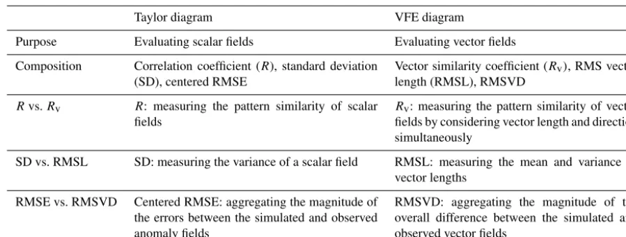
Table 1.Summary of the difference between the Taylor diagram and the VFE diagram.
Taylor diagram VFE diagram
Purpose Evaluating scalar fields Evaluating vector fields
Composition Correlation coefficient (R), standard deviation (SD), centered RMSE
Vector similarity coefficient (Rv), RMS vector length (RMSL), RMSVD
Rvs.Rv R: measuring the pattern similarity of scalar fields
Rv: measuring the pattern similarity of vector fields by considering vector length and direction simultaneously
SD vs. RMSL SD: measuring the variance of a scalar field RMSL: measuring the mean and variance of vector lengths
RMSE vs. RMSVD Centered RMSE: aggregating the magnitude of the errors between the simulated and observed anomaly fields
RMSVD: aggregating the magnitude of the overall difference between the simulated and observed vector fields
Figure 5.Diagram for displaying pattern statistics. The vector sim-ilarity coefficient between vector fields is given by the azimuthal position of the test field. The radial distance from the origin is pro-portional to the RMS length. The RMSVD between the test and ref-erence field is proportional to their distance apart (dashed contours in the same units as the RMS length).
5 Applications of the VFE diagram
5.1 Evaluating vector winds simulated by multiple models
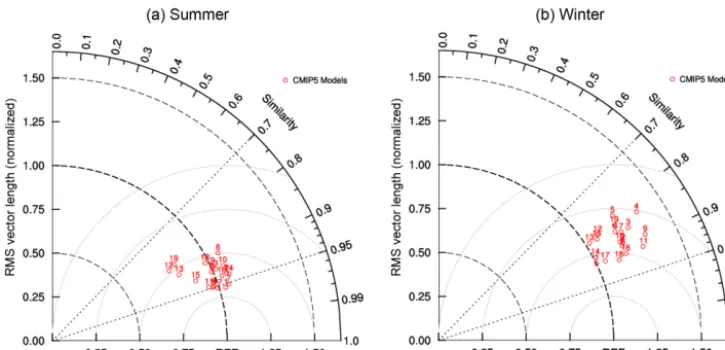
A common application of the VFE diagram is to com-pare multimodel simulations against observations in terms of the patterns of vector fields. As an example, we assess the pattern statistics of climatological mean 850 hPa vec-tor winds derived from the hisvec-torical experiments by 19 CMIP5 models (Taylor et al., 2012) compared with the NCEP-DOE Reanalysis 2 data during the period from 1979 to 2005. The evaluation was based on the monthly mean datasets from the first ensemble run of CMIP5 historical simulations and all datasets were regridded to a common grid of 2.5◦×2.5◦. A box-averaging (bi-linear interpolation)
method was used to regrid the reanalysis data and model data to a coarse (finer) resolution. The RMSVD and RMSL (LA
andLB)were normalized by the observed RMSL (LB), i.e.,
RMSVD0=RMSVD/LB,L0A=LA/LB, andL0B=1. This
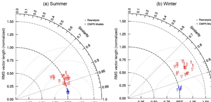
leaves VSC unchanged and yields a normalized diagram as shown in Fig. 6. The normalized diagram removes the units of variables and thus allows different variables to be shown in the same plot. The VSCs vary from 0.8 to 0.96 among 19 models, clearly indicating which model-simulated patterns of vector winds resemble observations well and which do not. The diagram also clearly shows which models overes-timate or underesoveres-timate the RMS wind speed (Fig. 6). For example, in comparison with the reanalysis data, some mod-els (e.g., 12, 19, 13, and 15) underestimate RMS wind speed characterized by smaller normalized RMSLs over the Asian– Australian monsoon region in summer. In contrast, some models (e.g., 6 and 10) overestimate wind speed (Fig. 6a). In winter, most models overestimate the 850 hPa RMS wind speed characterized greater normalized RMSLs (Fig. 6b).
To illustrate the performance of the VFE diagram in model evaluation, Fig. 7 shows the spatial patterns of the climatological mean 850 hPa vector winds over the Asian– Australian monsoon region derived from the NCEP2 reanal-ysis and three climate models. Models 1 and 4 show a spatial pattern of vector winds that is very similar to the reanaly-sis data in summer, andRv reaches 0.96 and 0.95,
respec-tively (Fig. 7a, c, e). In contrast, the spatial pattern of the vector winds simulated by model 12 is less similar to the re-analysis data (Fig. 7a, g). For example, the rere-analysis-based vector winds show stronger southwesterly winds over the southwestern Arabian Sea than the Bay of Bengal (Fig. 7a). However, an opposite spatial pattern is found in the same areas in model 12. More precisely, the southwesterly winds are weaker over the southwestern Arabian Sea than over the Bay of Bengal (Fig. 7g). Rv reasonably gives expression
Figure 6.Normalized pattern statistics of climatological mean 850 hPa vector winds in the Asian–Australian monsoon region (10◦S–40◦N, 40–140◦E) in summer (June–July–August) and winter (December–January–February) among 19 CMIP5 models compared with the NCEP Reanalysis 2 data during the period from 1979 to 2005. The RMS length and the RMSVD have been normalized by the RMS length derived from NCEP2. The data were excluded from the statistics in areas with a topography higher than 1500 m.
is clearly lower than that (0.96) in model 1. Figure 6 sug-gests that model 12 underestimates RMS wind speed (nor-malized RMS wind speed is 0.78) in summer. In contrast, model 4 overestimates RMS wind speed (normalized RMS wind speed is 1.35) in winter. These biases in wind speed can be identified in Fig. 7. For example, model 12 generally underestimates the 850 hPa wind speed, especially over the Somali region in summer, compared with the reanalysis data (Fig. 7a, g). Model 4 overestimates the strength of easterly winds between 5 and 20◦N and westerly winds between the Equator and 10◦S in winter (Fig. 7b, f).
5.2 Other potential applications
Similar to the Taylor diagram (Taylor, 2001), the VFE dia-gram can be applied to the following aspects.
5.2.1 Tracking changes in model performance
To summarize the changes in the performance of a model, the points on the VFE diagram can be linked with arrows. For example, similar to Fig. 5 in Taylor (2001) the tails of the arrows represent the statistics for the older version, and the arrowheads point to the statistic for the newer version of the model. By doing so, the multiple statistical changes from the old version to the new version of the model can be clearly shown in the VFE diagram. The VFE diagram can also be combined with the Taylor diagram to show the statis-tics for both scalar and vector variables in one diagram by plotting double coordinates because both diagrams are con-structed based on the law of cosine.
5.2.2 Indicating the statistical significance of differences in model performance
Figure 7.Climatological mean 850 hPa vector winds in summer and winter for the NCEP Reanalysis 2 data and the results of historical simulations obtained from three CMIP5 models during the period from 1979 to 2005. The vector similarity coefficient (Rv), normalized RMSL, and normalized RMSVD are also shown at the top of each panel. The vectors are set to a missing value in the areas with a topography higher than 1500 m.
the spatial pattern of vector winds (Fig. 8). The ensemble member involved here is less than 10 and the statistics be-tween models 12 and 13 are separated from each other by only a small distance on the VFE diagram, which may not be sufficient to conclude a significant difference between mod-els 12 and 13. This is a shortcoming of this method, i.e., lack-ing quantitative evaluation on the significance of difference in model performance, and warrants further study. Specif-ically, it may hard to determine the significance when the pattern statistics of two groups of simulations are not clearly separated from each other.
5.2.3 Evaluating model skill
Figure 8. Normalized pattern statistics for climatological mean 850 hPa vector winds over the Asian–Australian monsoon region (10◦S–40◦N, 40–140◦E) in summer (June–July–August) derived from each independent ensemble member by models 12, 13, and 14. The datasets used and regridding method are the same as those in Fig. 6, except only three models are included here. Models 12, 13, and 14 include 5, 6, and 9 ensemble simulations which are obtained from CMIP5 historical experiments during the period from 1979 to 2005, respectively. The same type of symbols show a close cluster-ing, and different types of symbols are clearly separated from each other, which suggests that the differences between different models are likely to be significant.
Sv1=
4(1+Rv)
(LA/LB+LB/LA)2(1+R0)
(14)
Sv2=
4(1+Rv)4
(LA/LB+LB/LA)2(1+R0)4
, (15)
whereR0 is the maximum VSC attainable.LA andLB are
the modeled and observed RMSL, respectively. Sv1or Sv2
take values between 0 (least skillful) and 1 (most skillful). Both skill scores can be shown as isolines in the VFE dia-gram, similar to Figs. 10 and 11 in Taylor (2001). For a given LA/LB, the skill increases linearly withRv. For a givenRv,
the skill is proportional (inversely proportional) toLA when
LA is smaller (greater) thanLB. Both skill scores,Sv1and
Sv2, take the VSC and the RMSL into account. However,
Sv1 places more emphasis on the correct simulation of the
vector length, whereas Sv2 pays more attention to the
pat-tern similarity of the vector fields. Which statistical variable is more important depends on the application. For example, wind speed (measured by RMSL) may be the primary con-cern of model evaluation if one evaluates models for the pur-pose of wind power projection. In contrast, the pattern of vector winds (measured by VSC) may be the major concern
Figure 9. Normalized pattern statistics of climatological mean 850 hPa vector winds in the Asian–Australian monsoon region (10◦S–40◦N, 40–140◦E) among 19 CMIP5 models compared with the reanalysis data in summer (June–July–August). The climato-logical means were computed from the monthly data derived from CMIP5 historical simulations and reanalysis datasets during the pe-riod from 1979 to 2005, except for the ERA-40 reanalysis with a time span from 1979 to 2002. Each CMIP5 model was compared with six reanalysis data, respectively. The symbols with same type of mark and color represent the statistics of an individual CMIP5 model compared with various reanalysis winds.
if one evaluates model performance in simulating monsoon climate. The users should define or select appropriate skill scores based on their own applications because no skill score would be universally considered most appropriate.
6 The impact of observational uncertainty on model evaluation
Figure 10.Normalized pattern statistics of climatological mean 850 hPa vector winds in the Asian–Australian monsoon region (10◦S–40◦N, 40–140◦E) derived from the historical simulations of 19 CMIP5 models (red circles) and 6 reanalysis datasets (blue crosses) compared with the multi-reanalysis mean during the period from 1979 to 2005. The RMSL and the RMSVD have been normalized by the RMSL derived from multi-reanalysis mean data. The data were excluded from the statistics in areas with topography higher than 1500 m. Six reanalysis datasets (NNRP, NCEP2, ERA-40, ERA-Interim, JRA25, and JRA55) were included in the statistics.
2011), JRA25 (Onogi et al., 2007), and JRA55 (Kobayashi et al., 2015; Harada et al., 2016) are observational data here. The modeled pattern statistics against various reanal-ysis datasets are similar to each other, indicating that the ob-servational uncertainty in vector winds has a minor impact on the evaluation of simulated climatological mean 850 hPa vector winds.
Note that the pattern statistics are less discriminable in Fig. 9 due to the overlapping of many symbols, although we use different symbols and colors to distinguish them from each other. To make the pattern statistics more clear, we pro-pose an alternative way to show the observational uncertainty by comparing each model and observation with the mean of multiple observational estimates. If we assume various ob-servational estimates are obtained independently and contain random noises, these noises can contaminate the observa-tional estimate. The random noises in various observaobserva-tional estimates could cancel out each other to a certain degree. Thus, the mean of multiple observational estimates may be closer to the true value than the individual observational esti-mate. We therefore take the ensemble mean of six reanalysis datasets as reference data and compute the pattern statistics of various models compared with the reference data to assess the model performance. Likewise, we can also measure the observational uncertainty by computing the pattern statistics of individual observational estimates relative to the reference data. The pattern statistics derived from models and individ-ual observations can be shown on the VFE diagram with dif-ferent symbols (Fig. 10). By doing so, one can roughly esti-mate the impacts of observational uncertainty on the evalu-ation of model performance. For example, the six reanalysis datasets show very close pattern statistics in summer charac-terized by high VSCs (0.986–0.994) and almost same
RM-SLs (0.986–1.021) as the reference data, which indicate a small observational uncertainty. Consequently, the observa-tional uncertainty should have less impact on the evaluation of model performance. This is further supported by the com-parison of Fig. 10 with Fig. 6. For example, the pattern statis-tics of CMIP5 models only show some minor changes when we replace the referenced NCEP-DOE Reanalysis 2 datasets with the ensemble mean of six reanalysis datasets (Figs. 6, 10).
7 Discussion and conclusions
evalu-ated (Figs. 6, 8). Alternatively, one can compute three sta-tistical variables using vector anomaly fields if the statistics in the anomaly are the primary concern. Under certain cir-cumstance, e.g., if the pattern of vector fields is highly ho-mogeneous, the statistics of full vector fields could largely be dominated by the mean vector fields with a minor contri-bution from the anomaly fields (Eqs. A1–A4). Consequently, the statistics derived from different models may be very sim-ilar and difficult to separate from each other. In this case, one may want to assess the mean and anomaly fields, re-spectively. By doing so, the model performance in simulating vector anomaly fields can be better identified on the VFE di-agram. The VFE diagram is devised to compare the statistics between two vector fields, e.g., vector winds usually com-prise two- or three-dimensional vectors. One-dimensional vector fields can be regarded as scalar fields. In terms of the one-dimensional case, the VSC, RMSL, and RMSVD computed by anomaly fields become the correlation coeffi-cient, standard deviation, and centered RMSE, respectively, and they are the statistical variables in the Taylor diagram. Thus, the Taylor diagram is a specific case of the VFE dia-gram. The Taylor diagram compares the statistics of scalar anomaly fields. The VFE diagram is a generalized Taylor di-agram that can compare the statistics of full vector fields or vector anomaly fields.
In practice, one may want to take latitudinal weight into account in the evaluation of spatial patterns of vector fields. This can be easily done by weighting the modeled and ob-served vector fields before computing VSC, RMSL, and RMSVD. Note that weighting should not be used during the computations of VSC, RMSL, and RMSVD to maintain their cosine relationship (Eq. 13). The VFE diagram can also be easily applied to the evaluation of three-dimensional vectors; however, we only considered two-dimensional vectors in this paper. If the vertical scale of a three-dimensional vector vari-able is much smaller than its horizontal scale, e.g., vector winds, one may consider multiplying the vertical component by 50 or 100 to accentuate its importance. In addition, as with the Taylor diagram, the VFE diagram can also be applied to track changes in model performance, indicate the signifi-cance of the differences in model performance, and evaluate model skills. More applications of the VFE diagram could be developed based on different research aims in the future.
8 Code availability
Appendix A: The relationship between the VFE diagram and the Taylor diagram
AandB:
Ai=(xai, yai);i=1,2, . . ., N Bi=(xbi, ybi);i=1,2, . . ., N .
AiandBiare two-dimensional vectors. Each full vector field
includesN vectors and can be broken down into the mean and anomaly:
Ai=A+A0i= xa+xai0 , ya+y 0 ai
;i=1,2, . . ., N
Bi=B+B0i= xb+xbi0 , yb+y 0 bi
;i=1,2, . . ., N , where xa=N1
N
P
i=1
xai, ya=N1 N
P
i=1
yai, xb=N1 N
P
i=1
xbi, yb=
1 N
N
P
i=1
ybi,A¯ = xa, ya
,B¯ = xb, yb
,A0i =
xai0 , yai0 ,Bi0 = xbi0 , ybi0 .
The standard deviation of thex andycomponents of vec-torsAi andBi can be written as follows:
σax=
v u u t 1 N N X
i=1
(xai−xa)2=
v u u t 1 N N X
i=1
x0ai2,
σay=
v u u t 1 N N X
i=1
yai−ya
2 = v u u t 1 N N X
i=1
yai0 2
σbx=
v u u t 1 N N X
i=1
(xbi−xb)2=
v u u t 1 N N X
i=1
xbi0 2,
σby=
v u u t 1 N N X
i=1
ybi−yb
2= v u u t 1 N N X
i=1
ybi0 2 .
The RMSL of vector fieldAis written as follows: L2A= 1
N
N
X
i=1
|Ai|2
= 1 N
N
X
i=1
xa+xai0
2
+ ya+yai0 2
= 1 N
N
X
i=1
x2a+ya2+ 1 N
N
X
i=1
x0ai2+yai0 2
+1 N
N
X
i=1
2xaxai0 +2yay 0 ai . Given N P
i=1
xai0 =
N
P
i=1
yai0 =0,L2Acan be written as
L2A= 1 N
N
X
i=1
Ai 2 + 1 N N X
i=1
A 0 i 2
=L2
A+L 2 A0
, (A1)
whereL2
A= 1 N
N
P
i=1
A¯
2
,L2A0=N1 N
P
i=1
A0i
2
. Similarly, we have
L2B=L2
B+L 2
B0. (A2)
The VSC between vector fieldsAandBis Rv=
1 s
N
P
i=1
|Ai|2
s
N
P
i=1
|Bi|2 N
X
i=1 Ai•Bi
= 1 N LALB
N
X
i=1
xa+xai0
xb+xbi0
+ ¯ya+yai0
¯ yb+ybi0
.
Given
N
P
i=1
xai0 =
N
P
i=1
yai0 =0, we obtain
Rv=
1 N LALB
N
X
i=1
(x¯ax¯b+ ¯yay¯b)+ x0aix 0 bi+y
0 aiy 0 bi = 1 N LALB
N
X
i=1
A•B+
N
X
i=1 A0i•B0i
!
=LALB LALB
Rv+
LA0LB0 LALB
Rv0 ,
(A3) where Rv=N L1
ALB
N
P
i=1
A•B= A•B
LALB = A•B
A B equals the cosine of the included angle between two mean vectors. Rv0= 1
N LA0LB0 N
P
i=1
A0i•B0i is the VSC between two vector anomaly fields.
The RMSVD2between vector fieldsAandBis
RMSVD2= 1 N
N
X
i=1
|Ai−Bi|2
= 1 N
N
X
i=1
¯
xa+xai0 − ¯xb−xbi0
2
+ ¯ya+y0ai− ¯yb−y0bi
2
= 1 N
N
X
i=1
(x¯a− ¯xb)2+(y¯a− ¯yb)2+ xai0 −x 0 bi
2+
yai0 −ybi0 2
= 1 N
N
X
i=1
A−B
2 + 1 N N X
i=1
A0i−B0i
2
.
(A4) Based on Eqs. (A1), (A2), and (A4), we can conclude that theLA,LB, and RMSVD2derived from the full vector fields
are equal to those derived from the mean vector fields plus those derived from the vector anomaly fields. TheRv
fields takes the statistics in both the mean state and anomaly of the vector fields into account. The VFE diagram derived from the full vector fields is recommended for use if both the statistics in the mean state and anomaly are of great con-cern. On the other hand, the VFE diagram derived from vec-tor anomaly fields can be used if the statistics in the anomaly are the primary concern. In this case, anomalousLA,LB,Rv,
and RMSVD2can be written, respectively, as follows:
L2A0= 1 N
N
X
i=1
A
0 i
2
= 1 N
N
X
i=1
(xai0 2+yai0 2) (A5)
L2B0 = 1 N
N
X
i=1
B0i
2
= 1 N
N
X
i=1
(xbi0 2+ybi0 2) (A6)
Rv0=
1 s
N
P
i=1
A0i
2
s
N
P
i=1
B0i
2 N
X
i=1 A0i•B0i
= 1
s
N
P
i=1
xai0 2+yai0 2 s
N
P
i=1
xbi0 2+ybi0 2
N
X
i=1
(xai0 xbi0 +yai0 ybi0 )
(A7) RMSVD2v0=
1 N
N
X
i=1
A
0 i−B
0 i
2
= 1 N
N
X
i=1
xai0 −xbi0 2+ yai0 −ybi0 2. (A8)
The vector fieldsAandB can be regarded as two scalar fields if we further assume that theycomponent of both vec-tor fields is equal to 0. Under this circumstance, Eqs. (A5)– (A8) can be written as follows:
L2A0= 1 N
N
X
i=1
xai0 2=σax2
L2B0= 1 N
N
X
i=1
xbi0 2=σbx2
Rv0=
1 s
N
P
i=1
xai0 2 s
N
P
i=1
xbi0 2
N
X
i=1
xai0 xbi0
RMSVD2v0 = 1 N
N
X
i=1
xai0 −xbi0 2 .
LA0 and LB0 are equal to the standard deviation of the xcomponent of vector fieldsAandB, respectively.R0
vis the
Pearson’s correlation coefficient between thexcomponent of vector fieldsAandB, and RMSVD2v0 is the centered RMS difference between thex component of vector fieldsAand
The Supplement related to this article is available online at doi:10.5194/gmd-9-4365-2016-supplement.
Author contributions. Z. Xu and Z. Hou are the first coauthors. Z. Xu constructed the diagram and led the study. Z. Hou and Z. Xu performed the analysis. Z. Xu and Y. Han wrote the paper. All of the authors discussed the results and commented on the manuscript.
Acknowledgements. We acknowledge the World Climate Research Programme’s Working Group on Coupled Modelling, which is responsible for CMIP, and we thank the climate modeling groups for producing and making their model output available. NCEP/NCAR Reanalysis 1 and NCEP-DOE Reanalysis 2 datasets were provided by the NOAA/OAR/ESRL PSD, Boulder, Colorado, USA, through their website at http://www.esrl.noaa.gov/psd/. The ERA-40 and ERA-Interim Reanalysis datasets were provided by the European Centre for Medium-Range Weather Forecasts (ECMWF). The JRA25 and JRA55 Reanalysis datasets were provided from the Japanese 25- and 55-year reanalysis projects carried out by the Japan Meteorological Agency (JMA). The study was supported jointly by the National Basic Research Program of China Project 2012CB956200, the National Key Technologies R&D Program of China (grant 2012BAC22B04), and the NSF of China grants (41675105, 41475063). This work was also supported by the Jiangsu Collaborative Innovation Center for Climate Change.
Edited by: K. Gierens
Reviewed by: two anonymous referees
References
Charles, B. N.: Utility of stretch vector correlation coefficients, Q. J. Roy. Meteor. Soc., 85, 287–290, doi:10.1002/qj.49708536510, 1959.
Chaudhuri, A. H., Ponte, R. M., Forget, G., and Heimbach, P.: A comparison of atmospheric reanalysis surface products over the ocean and implications for uncertainties in air–sea boundary forcing, J. Climate, 26, 153–170, 2013.
Crosby, D. S., Breaker, L .C., and Gemmill, W. H.: A proposed definition for vector correlation in geophysics: Theory and appli-cation, J. Atmos. Ocean. Tech., 10, 355–367, 1993.
Dee, D. P., Uppala, S. M., Simmons A. J., Berrisford, P., Poli, P., Kobayashi, S., Andrae, U., Balmaseda, M. A., Balsamo, G., Bauer, P., Bechtold, P., Beljaars, A. C. M., van de Berg, L., Bid-lot, J., Bormann, N., Delsol, C., Dragani, R., Fuentes, M., Geer, A. J., Haimberger, L., Healy, S. B., Hersbach, H., Hólm, E. V., Isaksen, L., Kållberg, P., Köhler, M., Matricardi, M., McNally, A. P., Monge-Sanz, B. M., Morcrette, J.-J., Park, B.-K., Peubey, C., de Rosnay, P., Tavolato, C., Thépaut, J.-N., and Vitart, F.: The ERA-Interim reanalysis: configuration and performance of the data assimilation system, Q. J. Roy. Meteor. Soc., 137, 553–579, 2011.
Ellison, T. H.: On the correlation of vectors, Q. J. Roy. Meteor. Soc., 80, 93–96, doi:10.1002/qj.49708034311, 1954.
Giorgi, F. and Gutowski, W. J.: Regional Dynamical Downscaling and the CORDEX Initiative, Annu. Rev. Environ. Res., 40, 467– 490, 2015.
The HadGEM2 Development Team: Martin, G. M., Bellouin, N., Collins, W. J., Culverwell, I. D., Halloran, P. R., Hardiman, S. C., Hinton, T. J., Jones, C. D., McDonald, R. E., McLaren, A. J., O’Connor, F. M., Roberts, M. J., Rodriguez, J. M., Woodward, S., Best, M. J., Brooks, M. E., Brown, A. R., Butchart, N., Dear-den, C., Derbyshire, S. H., Dharssi, I., Doutriaux-Boucher, M., Edwards, J. M., Falloon, P. D., Gedney, N., Gray, L. J., Hewitt, H. T., Hobson, M., Huddleston, M. R., Hughes, J., Ineson, S., In-gram, W. J., James, P. M., Johns, T. C., Johnson, C. E., Jones, A., Jones, C. P., Joshi, M. M., Keen, A. B., Liddicoat, S., Lock, A. P., Maidens, A. V., Manners, J. C., Milton, S. F., Rae, J. G. L., Rid-ley, J. K., Sellar, A., Senior, C. A., Totterdell, I. J., Verhoef, A., Vidale, P. L., and Wiltshire, A.: The HadGEM2 family of Met Of-fice Unified Model climate configurations, Geosci. Model Dev., 4, 723–757, doi:10.5194/gmd-4-723-2011, 2011.
Hanson, B., Klink, K., Matsuura, K., Robeson, S. M., and Will-mott, C. J.: Vector correlation: Review, Exposition, and Geo-graphic Application, Annals of the Association of American Ge-ographers, 82, 103–116, 1992.
Harada, Y., Kamahori H., Kobayashi C., Endo, H., Kobayashi, S., Ota, Y., Onoda, H., Onogi, K., Miyaoka, K., and Takahashi, K.: The JRA-55 Reanalysis: Representation of atmospheric circula-tion and climate variability, J. Meteor. Soc. Jpn., 94, 269–302, doi:10.2151/jmsj.2016-015, 2016.
Hellström C., and Chen, D.: Statistical Downscaling Based on Dy-namically Downscaled Predictors: Application to Monthly Pre-cipitation in Sweden, Adv. Atmos. Sci., 20, 951–958, 2003. Jiang, Z., Li, W., Xu, J., and Li, L.: Extreme Precipitation Indices
over China in CMIP5 Models. Part I: Model Evaluation, J. Cli-mate, 28, 8603–8619, 2015.
Jupp P. E. and Mardia K. V.: A general correlation coefficient for directional data and related regression problems, Biometrika, 67, 163–173, 1980.
Kalnay, E., Kanamitsu, M., Kistler, R., Collins, W., Deaven, D., Gandin, L., Iredell, M., Saha, S., White, G., and Woollen, J.: The NCEP/NCAR 40-year reanalysis project, B. Am. Meteorol. Soc., 77, 437–470, 1996.
Kanamitsu, M., Ebisuzaki, W., Woollen J., Yang, S.-K., Hnilo, J. J., Fiorino, M., and Potter, G. L.: NCEP-DOE AMIP-II Reanalysis (R-2), B. Am. Meteorol. Soc., 83, 1631–1643, 2002.
Katragkou, E., García-Díez, M., Vautard, R., Sobolowski, S., Za-nis, P., Alexandri, G., Cardoso, R. M., Colette, A., Fernandez, J., Gobiet, A., Goergen, K., Karacostas, T., Knist, S., Mayer, S., Soares, P. M. M., Pytharoulis, I., Tegoulias, I., Tsikerdekis, A., and Jacob, D.: Regional climate hindcast simulations within EURO-CORDEX: evaluation of a WRF multi-physics ensemble, Geosci. Model Dev., 8, 603–618, doi:10.5194/gmd-8-603-2015, 2015.
Kobayashi, S., Ota, Y., Harada, Y., Ebita, A., Moriya, M., Onoda, H., Onogi, K., Kamahori, H., Kobayashi, C., and Endo, H.: The JRA-55 Reanalysis: General specifications and basic characteris-tics, J. Meteor. Soc. Jpn., 93, 5–48, doi:10.2151/jmsj.2015-001, 2015.
Lamberth, R. L.: On the Use of Court’s Versus Durst’s Techniques for Computing Vector Correlation Coefficients, J. Appl. Meteo-rol., 5, 736–737, 1966.
Lee, T., Waliser, D. E., Li, J.-L., Landerer, F. W., and Gierach, M. M.: Evaluation of CMIP3 and CMIP5 Wind Stress Climatol-ogy Using Satellite Measurements and Atmospheric Reanalysis Products, J. Climate, 26, 5810–5826, 2012.
Onogi, K., Tsutsui J., Koide H., Sakamoto, M., Kobayashi, S., Hat-sushika, H., Matsumoto, T., Yamazaki, N., Kamahori, H., and Takahashi, K.: The JRA-25 Reanalysis, J. Meteor. Soc. Jpn., 85, 369–432, 2007.
Shukla, J. and Saha, K. R.: Computation of non-divergent stream function and irrotational velocity potential from the observed winds, Mon. Weather Rev., 102, 419–425, 1974.
Sperber, K. R., Annamalai, H., Kang, I. S., Kitoh, A., Moise, A., Turner, A., Wang B., and Zhou, T.: The Asian summer monsoon: an intercomparison of CMIP5 vs. CMIP3 simula-tions of the late 20th century, Clim. Dynam., 41, 2771–2744, doi:10.1007/s00382- 012-1607-6, 2013.
Stephens, M. A.: Vector correlation, Biometrika, 66, 41–48, 1979. Taylor, K. E.: Summarizing multiple aspects of model performance
in a single diagram, J. Geophys. Res.-Atmos., 106, 7183–7192, 2001.
Taylor, K. E., Stouffer, R. J., and Meehl G. A.: An Overview of CMIP5 and the experiment design, B. Am. Meteorol. Soc., 93, 485–498, doi:10.1175/BAMS-D-11-00094.1, 2012.
Twardosz, R. Nied´zwied´z, T., and Łupikasza, E.: The influence of atmospheric circulation on the type of precipitation (Kraków, southern Poland), Theor. Appl. Climatol., 104, 233–250, 2011. Uppala, S. M., Kallberg, P. W., Simmons A. J., Andrae, U., Da
Costa Bechtold, V., Fiorino, M., Gibson, J. K., Haseler, J., Her-nandez, A., Kelly, G. A., Li, X., Onogi, K., Saarinen, S., Sokka, N., Allan, R. P., Andersson, E., Arpe, K., Balmaseda, M. A., Beljaars, A. C. M., Van De Berg, L., Bidlot, J., Bormann, N., Caires, S., Chevallier, F., Dethof, A., Dragosavac, M., Fisher, M., Fuentes, M., Hagemann, S., Hólm, E., Hoskins, B.J., Isaksen, L., Janssen, P. A. E. M., Jenne, R., McNally, A. P., Mahfouf, J. F., Morcrette, J.-J., Rayner, N. A., Saunders, R. W., Simon, P., Sterl, A., Trenberth, K. E., Untch, A., Vasiljevic, D., Viterbo, P., and Woollen, J.: The ERA-40 re-analysis, Q. J. Roy. Meteor. Soc., 131, 2961–3012, 2005.
Wei, J., Jin, Q., Yang, Z.-L., and Dirmeyer, P. A.: Role of ocean evaporation in California droughts and floods, Geophys. Res. Lett., 43, 6554–6562, doi:10.1002/2016GL069386, 2016. Zhou, T., Turner, A. G., Kinter, J. L., Wang, B., Qian, Y., Chen,