Vol 2013

ISSN 2307-7743 http://scienceasia.asia

_______________

2010 Mathematics Subject Classification: 90C29.

Key words and phrases: Differential transformation method (DTM), free vibration, uniform beams, nonuniform beams.

©2013 Science Asia 1 / 16

FREE VIBRATION OF UNIFORM AND NON-UNIFORM EULER BEAMS USING

THE DIFFERENTIAL TRANSFORMATION METHOD

MAHMOUD A. A., ABDELGHANY S. M., EWIS K. M.

Abstract. In this paper, the differential transformation method (DTM) is applied for free vibration analysis of beams with uniform and non-uniform cross sections. Natural frequencies and corresponding normalized mode shapes are calculated for different cases of cross section and boundary conditions. MATLAB code is designed to solve the differential equation of the beam using the differential transformation method. Comparison of the present results with the previous solutions proves the accuracy and versatility of the presented paper.

1.

In order to calculate fundamental natural frequencies and the corresponding mode shapes, different variational techniques such as Rayleigh_Ritz and Galerkin methods had been applied in the past. Besides these techniques, another numerical methods were also successfully applied to beam vibration analysis such as finite element method.

propagation of magnetic flux and stability of fluid motions. J. Biazar and M. Eslami [8] used DTM for Nonlinear Parabolic-hyperbolic Partial differential equations. DTM was applied to linear and nonlinear system of ordinary differential equations by Farshid Mirzaee [9]. Keivan Torabi et al. [10] applied DTM for longitudinal vibration analysis of beams with non-uniform cross section. The non-linear vibration analysis of beams is applied by Qiang Guo and Hongzhi Zhong [11] using a spline-based differential quadrate method.

In this paper, the vibration problems of uniform and non-uniform Euler-Bernoulli beams have been solved analytically using DTM for various end conditions.

2.

Following ref [2] we can obtain the idea of the DTM, The differential transformation of function u(x) is defined as follows;

0

1 ( )

( ) !

k

k x

d u x U k

k dx ₌

 

= _{ }

  (1)

In Eq. (1), u(x) is the original function and U(k) is the transformed function. Differential inverse transform of U(k) is defined as follows;

0

( ) k ( )

k

u x x U k

∞

=

=

∑

In fact, from (1) and (2), we obtain

0 ₀

( ) ( )

!

k k

k

x _x

x d u x u x

k dx

∞

= ₌

 

= _{ }

 

∑

Eq. (3) implies that the concept of differential transformation is derived from the Taylor series expansion. From the definitions (1) and (2), it is easy to obtain the following mathematical operations; [2, 3, 4, 6, 9]

1. If f x( )=g x( )±h x( ), then F k( )=G k( )±H k( ).

3. If ( ) ( ),

n

n

d g x f x

dx

= _then ( ) ( )! ( ).

!

k n

F k G k n

k

+

= +

4. If f x( )=g x h x( ) ( ), then

0

( ) ( ) ( ).

k

l

F k G l H k l

=

=

∑

5. If f x( )=xn, then F k( )=δ(k−n), δ is the Kronecker delta.

7. If ( ) (1 ) ( )

n m

n

d g x f x a bx

dx

= − _then

0

( )!

( ) ( ) ( )

( )!

m m

r r

r

C k n r

F k a b G k n r

k r =

+ −

= − + −

−

∑

b are constants

3.

Free Vibration of a Non-uniform Beam

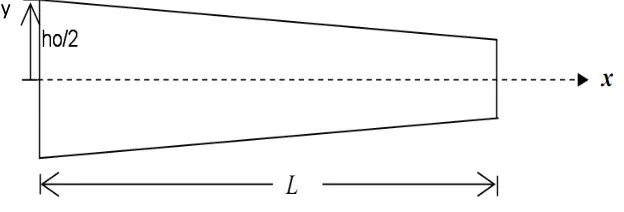
The governing differential equation for a non-uniform Euler beam shown in fig. 1 is given by:

2 2 2

2 2 2

( , ) ( , )

( ) v x t ( ) v x t 0

A x EI x

t x x

ρ ∂ + ∂ _ ∂ _=

∂ ∂ _ ∂ _ (4)

Where ρ is the density of the beam material, A x( )is the cross sectional area of the beam, ( , )

v x t is displacement of the beam, I x( )is the inertia at distance x from the left end of the

beam and E is young’s modulus of the beam.

Figure 1 Beam with variable cross-section

Boundary conditions:

Case a. Simple –Simple Beam

(0, ) 0

v t = ;

2 2 (0, )

0

v t x

∂ ₌

∂ ; v L t( , )=0;

2 2 ( , )

0

v L t x

∂ ₌

∂ (5)

Case b. Clamped- Clamped Beam

(0, ) 0

v t = ; v(0, )t 0 x

∂ ₌

∂ ; v L t( , )=0;

( , ) 0 v L t

x

∂ ₌

∂ (6)

Case c. Clamped- Roller Beam

(0, ) 0

v t = ; v(0, )t 0 x

∂ ₌

∂ ; v L t( , )=0;

2 2 ( , )

0

v L t x

∂

=

∂ (7)

Where L is the beam length and t is the time

4.

Assume that, the displacement of the beam is given by:

( , ) ( ) exp( )

v x t =v x i tω (8)

Where ω is the natural frequency of the beam.

Equation (4) can be conveniently written as :

4 3 2 2

2

4 3 2 2

( )

( )

( )

( )

( )

( )

( )

d v x

2

dI x d v x

d I x d v x

0

A x

v x

E

E

E

dx

dx

dx

dx

dx

ρ

ω

With boundary conditions as,

Case a. Simple –Simple Beam

(0) 0

v = ;

2 2 (0)

0

d v

dx = ; v L( )=0;

2 2 ( )

0

d v L

dx = (10)

Case b. Clamped- Clamped Beam

(0) 0

v = ; dv(0) 0

dx = ; v L( )=0; ( )

0 dv L

dx = (11)

Case c. Clamped- Roller Beam

(0) 0

v = ; dv(0) 0

dx = ; v L( )=0;

2 2 ( )

0

d v L

dx = (12)

5.

Equations (9) can be conveniently written in terms of dimensionless variables as :

4 3 2 2

2 1/3

4 3 2 2

( ) ( ) ( ) ( ) ( )

( )d y x 2dS x d y x d S x d y x ( ( )) ( )

S x S x y x

dx + dx dx + dx dx = Ω (13)

where

3

0

( )

( )

(1

)

EI x

S x

x

EI

=

= −

β

,

v

y

L

=

x

x

L

=

1/3

0

( )

( )

A x

S

x

A

=

1/3

0

( )

( )

h x

(1

)

S

x

x

h

β

4

2 0

0

A L

EI

ρ

ω

Ω =

h

, ,

A

I

beam height , the cross sectional area and the inertia at the point at the left edge of the beam, and

β

the non-dimensional boundary conditions are,

Case a. Simple –Simple Beam

(0) 0

y = ;

2 2 (0)

0

d y

dx = ; y(1)=0;

2 2 (1)

0

d y

dx = (14)

Case b. Clamped- Clamped Beam

(0) 0

y = ; dy(0) 0

dx = ; y(1)=0;

(1) 0

dy

dx = (15)

Case c. Clamped- Roller Beam

(0) 0

y = ; dy(0) 0

dx = ; y(1)=0;

2 2 (1)

0

d y

dx = (16)

6.

[

]

[

]

( 1)( )( 1)( 2) 6 ( 1)( 2) 6( 1)( 2)

1

( 1)( 2)( 3)( 4) 2 ( 1)( 2)( 3) 3( 1)( 2)( 3)

k k

k

k

Y k k k k k k k k k Y

Y

k k k k k k k k k k k Y

β β

+ +

+

Ω − − + + + + + + + + 

 

= _{ }

+ + + + _+ + + + + + + + _

(17)

Then applying the Differential Transform Method to the non-dimensional boundary conditions equations (14)-(16) yield,

Case a. Simple –Simple Beam

The DT of Eqs. (14) is written as

y(0)= 0 1 2 3 4 5

0

[ ] k [0] [1] [2] [3] [4] [5] ... 0

k

Y k x Y x Y x Y x Y x Y x Y x

∞

=

= + + + + + + =

∑

leads to Y[0]=0 (18.a)

'' 0 1 2

0

3 4 5

(0) ( 1)( 2) [ 2] (1)(2) [2] (2)(3) [3] (3)(4) [2]

(4)(5) [3] (5)(6) [4] (6)(7) [5] ... 0

k

k

y k k Y k x Y x Y x Y x

Y x Y x Y x

∞

=

= + + + = + +

+ + + + =

∑

leads to Y[2]=0 (18.b)

y(1)= 0 1 2 3 4 5

0

[ ] k [0] [1] [2] [3] [4] [5] ... 0

k

Y k x Y x Y x Y x Y x Y x Y x

∞ = = + + + + + + =

∑

[ ] 0

k

Y k

∞

=

=

∑

Taking Y[1]=c (18.d)

'' 0 1 2

0

3 4 5

(1) ( 1)( 2) [ 2] (1)(2) [2] (2)(3) [3] (3)(4) [2]

(4)(5) [3] (5)(6) [4] (6)(7) [5] ... 0

k

k

y k k Y k x Y x Y x Y x

Y x Y x Y x

∞ = = + + + = + + + + + + =

∑

( 1) [ ] 0

k

k k Y k

∞

=

− =

∑

Equations (18.c) and (18.e) may be written as

1 1 1

1 1 1

0

0

aa bb c

cc dd d

      =      

 

    (19)

since c1 and d1 are not zero, for a non-trivial solution to exist the determinant of the matrix

must be zero, i.e.

1 1 1 1 0

aa ×dd −cc ×bb = (20)

where aa1, bb1 are the coefficients of c1 and d1 in the equation (18.c) and cc1, dd1 are the

coefficients of c1 and d1 in the equation (18.e). The root of Eq. (20) is the solution for case a

of the problem.

Case b. Clamped- Clamped Beam

The DT of Eqs. (15) is written as

y(0)= 0 1 2 3 4 5

0

[ ] k [0] [1] [2] [3] [4] [5] ... 0

k

Y k x Y x Y x Y x Y x Y x Y x

∞

=

= + + + + + + =

∑

leads to Y[0]=0 (21.a)

' 0 1 2 3

0

4 5

(0) ( 1) [ 1] (1) [1] (2) [2] (3) [3] (4) [4]

+(5) [5] (6) [6] ... 0

k

k

y k Y k x Y x Y x Y x Y x

Y x Y x

∞

=

= + + = + + +

+ + =

∑

leads to Y[1]=0 (21.b)

y(1)= 0 1 2 3 4 5

0

[ ] k [0] [1] [2] [3] [4] [5] ... 0

k

Y k x Y x Y x Y x Y x Y x Y x

∞

=

= + + + + + + =

∑

leads to

0

[ ] 0

k

Y k

∞

=

=

∑

' 0 1 2 3 0

4 5

(1) ( 1) [ 1] (1) [1] (2) [2] (3) [3] (4) [4]

+(5) [5] (6) [6] ... 0

k

k

y k Y k x Y x Y x Y x Y x

Y x Y x

∞

=

= + + = + + +

+ + =

∑

leads to

0

[ ] 0

k

kY k

∞

=

=

∑

Taking Y[3]=d (21.f)

Equations (21.c) and (21.e) may be written as

2 2 2

2 2 2

0

0

aa bb c

cc dd d

      =      

 

    (22)

since c2 and d2 are not zero, for a non-trivial solution to exist the determinant of the matrix

must be zero, i.e.

2 2 2 2 0

aa ×dd −cc ×bb = (23)

where aa2, bb2 are the coefficients of c2 and d2 in the equation (21.c) and cc2, dd2 are the

coefficients of c2 and d2 in the equation (21.e). The root of Eq. (23) is the solution for case b

of the problem.

Case c. Clamped- Roller Beam

The DT of Eqs. (16) is written as

y(0)= 0 1 2 3 4 5

0

[ ] k [0] [1] [2] [3] [4] [5] ... 0

k

Y k x Y x Y x Y x Y x Y x Y x

∞

=

= + + + + + + =

∑

leads to Y[0]=0 (24.a)

' 0 1 2 3

0

4 5

(0) ( 1) [ 1] (1) [1] (2) [2] (3) [3] (4) [4]

+(5) [5] (6) [6] ... 0

k

k

y k Y k x Y x Y x Y x Y x

Y x Y x

∞

=

= + + = + + +

+ + =

∑

y(1)= 0 1 2 3 4 5 0

[ ] k [0] [1] [2] [3] [4] [5] ... 0

k

Y k x Y x Y x Y x Y x Y x Y x

∞

=

= + + + + + + =

∑

leads to

0

[ ] 0

k

Y k

∞

=

=

∑

Taking Y[2]=c (24.d)

'' 0 1 2

0

3 4 5

(1) ( 1)( 2) [ 2] (1)(2) [2] (2)(3) [3] (3)(4) [2]

(4)(5) [3] (5)(6) [4] (6)(7) [5] ... 0

k

k

y k k Y k x Y x Y x Y x

Y x Y x Y x

∞

=

= + + + = + +

+ + + + =

∑

leads to

0

( 1) [ ] 0

k

k k Y k

∞

=

− =

∑

Taking Y[3]=d (24.f)

Equations (24.c) and (24.e) may be written as

3 3 3

3 3 3

0

0

aa bb c

cc dd d

      =      

 

    (25)

since c3 and d3 are not zero, for a non-trivial solution to exist the determinant of the matrix

must be zero, i.e.

3 3 3 3 0

aa ×dd −cc ×bb = (26)

where aa3, bb3 are the coefficients of c3 and d3 in the equation (24.c) and cc3, dd3 are the

coefficients of c3 and d3 in the equation (24.e). The root of Eq. (26) is the solution for case c

of the problem.

7.

For a beam with simply supported ends Ω2

= 97.4091 leads to the first non-dimensional natural frequency as Ω =9.8696, which agrees with closed form value [5].

For a beam with clamped supported ends, Ω2

For a beam with one end clamped and the other end free, Ω2

= 237.721 leads to the first non-dimensional natural frequency as Ω =15.4182, which agrees with closed form value

[5].

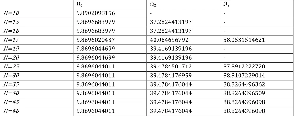
Table 1 compares the accuracy of the first three non-dimensional frequencies of Simply supported uniform beams for different number of terms N. It is observed that the convergence speed increases with decreasing frequency order. i.e, the first frequency Ω1

needs 25 terms to reach exact solution , while , third frequency Ω3 needs 45 terms. Table 2

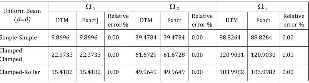
gives results of the first three non-dimensional frequencies of Euler beams with uniform cross section and different cases of boundary conditions. In table 2 exact values are also listed for direct comparison. It can be demonstrated that the differential transformation method is an efficient method in solving the vibrations of beams with good accuracy. Table 3 gives results of the first three dimensional frequencies of simply supported non-uniform Euler beams with different values of beta β . It can be demonstrated that the first three frequencies of the simply non-uniform beam decreases with increasing β due to decreasing the beam cross section. Tables 4 and 5 gives results of the first three non-dimensional frequencies of clamped-clamped and clamped-roller non-uniform Euler beams with different values of beta β which give different cross sections. It is also observed that the first three frequencies of the clamped-clamped and clamped-roller non-uniform beam decreases with decreasing of the cross section.

Table 1. The first three Non-dimensional frequencies of Simple-Simple uniform Euler Beams for different number of terms N

Ω1 Ω2 Ω3

N=10 9.8902098156 - -

N=15 9.8696683979 37.2824413197 - N=16 9.8696683979 37.2824413197 -

N=17 9.8696020437 40.064696792 58.0531514621 N=19 9.8696044699 39.4169139196 -

N=20 9.8696044699 39.4169139196 -

Table 2. Comparison of results for free vibration of uniform Euler beams. The first three Non-dimensional frequencies of uniform Euler Beams: Uniform Beam

(β=0)

Ω1 Ω2 Ω3

DTM Exact] Relative _{error %} DTM Exact Relative _{error %} DTM Exact Relative _{error %} Simple-Simple 9.8696 9.8696 0.00 39.4784 39.4784 0.00 88.8264 88.8264 0.00

Clamped-Clamped 22.3733 22.3733 0.00 61.6729 61.6728 0.00 120.9031 120.9030 0.00 Clamped-Roller 15.4182 15.4182 0.00 49.9649 49.9649 0.00 103.9982 103.9982 0.00

-The first three Non-dimensional frequencies of Non-uniform Euler Beams for different values of β:

Table 3. Simply supported Non-uniform Euler Beams

3 0

( )

(1 )

( ) EI x

x

EI x = −β

Ω1 Ω2 Ω3

β=0 β=0.25 β=0.5 β=0 β=0.25 β=0.5 β=0 β=0.25 β=0.5

Simple-Simple 9.8696 8.5772 7.1215 39.4784 34.4062 28.9519 88.8107 77.3785 64.9802

Table 4. Clamped-Clamped Non- uniform Euler Beams

3 0

( )

(1 )

( ) EI x

x

EI x = −β

Ω1 Ω2 Ω3

β=0 β=0.25 β=0.5 β=0 β=0.25 β=0.5 β=0 β=0.25 β=0.5

Clamped-Clamped 22.3733 19.4836 16.3356 61.6729 53.6971 44.9817 120.9031 105.2123 88.1593

Table 5. Clamped - Roller Non -uniform Euler Beams

3 0

( )

(1 )

( ) EI x

x

EI x = −β

Ω1 Ω2 Ω3

β=0 β=0.25 β=0.5 β=0 β=0.25 β=0.5 β=0 β=0.25 β=0.5

Clamped-Roller 15.4182 13.9524 12.3001 49.9649 44.0199 37.5276 103.9982 91.2744 77.1247

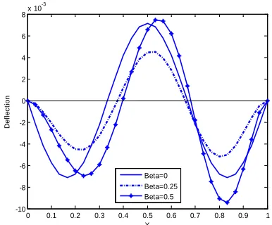
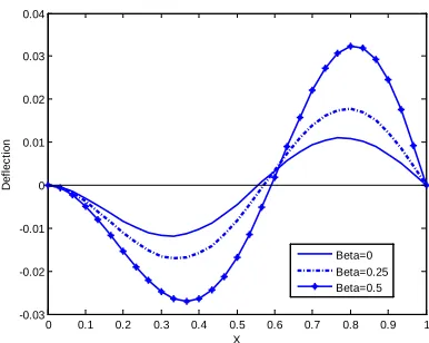
shapes drawn using DTM is very agreement with the mode shaped drawn using exact methods. Figures (5-7) show, respectively, the first, the second and the third mode shapes of simply supported non-uniform Euler beams with different cross sections. Also figures (8-13) show, respectively, the first, the second and the third mode shapes of clamped-clamped and clamped-clamped-roller non-uniform Euler beams with different cross sections. From figures (5-13)). It can be seen that the value of beta (β=0, 0.25 and 0.5) has a significant effect on the mode shapes and the deflection values. Deflection of non-uniform beams increases as cross section decreases (β values increases). For Euler beam with uniform cross section (β =0).

Fig. 2 The first three mode shapes of Simple –Simple

uniform-beam Fig. 3 The first three mode shapes of Clamped- _{Clamped uniform-beam}

Fig. 4 The first three mode shapes of Clamped-

Roller uniform beam Fig. 5 The first mode shapes for three different values _{of Beta of Simple –Simple non-uniform beam}

0 0.2 0.4 0.6 0.8 1

-0.2 -0.15 -0.1 -0.05 0 0.05

X

D

ef

lec

ti

on

DTM Exact First Mode

Third Mode Second Mode

0 0.2 0.4 0.6 0.8 1

-0.04 -0.035 -0.03 -0.025 -0.02 -0.015 -0.01 -0.005 0 0.005 0.01

X

D

ef

lec

ti

on

DTM Exact First Mode

Third Mode

Second Mode

0 0.2 0.4 0.6 0.8 1

-0.07 -0.06 -0.05 -0.04 -0.03 -0.02 -0.01 0 0.01 0.02

X

D

ef

lec

ti

on

DTM Exact First Mode

Second Mode

Third Mode

0 0.1 0.2 0.3 0.4 0.5 0.6 0.7 0.8 0.9 1 -0.3

-0.2 -0.1 0 0.1 0.2 0.3 0.4

X

D

ef

lec

ti

on

Fig. 6 The Second mode shapes for three different values of Beta of Simple –Simple non-uniform beam

Fig. 7 The Third mode shapes for three different values of Beta of Simple –Simple non-uniform beam

Fig. 8 The first mode shapes for three different values of Beta of Clamped-Clamped non-uniform beam

Fig. 9 The Second mode shapes for three different values of Beta of Clamped-Clamped non-uniform beam

Fig. 10 The Third mode shapes for three different values of Beta of Clamped-Clamped non-uniform beam

Fig. 11 The first mode shapes for three different values of Beta of Clamped- Roller non-uniform beam

0 0.1 0.2 0.3 0.4 0.5 0.6 0.7 0.8 0.9 1

-0.06 -0.04 -0.02 0 0.02 0.04 0.06 0.08 X D ef lec ti on Beta=0 Beta=0.25 Beta=0.5

0 0.1 0.2 0.3 0.4 0.5 0.6 0.7 0.8 0.9 1 -0.02 -0.015 -0.01 -0.005 0 0.005 0.01 0.015 0.02 X D ef lec ti on Beta=0 Beta=0.25 Beta=0.5

0 0.1 0.2 0.3 0.4 0.5 0.6 0.7 0.8 0.9 1 -0.06 -0.04 -0.02 0 0.02 0.04 0.06 0.08 0.1 0.12 X D ef lec ti on Beta=0 Beta=0.25 Beta=0.5

0 0.1 0.2 0.3 0.4 0.5 0.6 0.7 0.8 0.9 1 -0.03 -0.02 -0.01 0 0.01 0.02 0.03 X D ef lec ti on Beta=0 Beta=0.25 Beta=0.5

0 0.1 0.2 0.3 0.4 0.5 0.6 0.7 0.8 0.9 1 -10 -8 -6 -4 -2 0 2 4 6 8x 10

-3 X D ef lec ti on Beta=0 Beta=0.25 Beta=0.5

Fig. 12 The Second mode shapes for three different values of Beta of Clamped- Roller non-uniform beam

8.

Fig. 13 The Third mode shapes for three different values of Beta of Clamped- Roller non-uniform beam

Based on the results presented, it can be demonstrated that the differential transformation method is an efficient method in solving the vibrations of beams with good accuracy using a few terms. The frequency of non-uniform beam decreases with decreasing of the cross section area and its inertia. Also it is observed that the deflection of the non-uniform Euler beam is increased as the cross section is decreased.

REFERENCES

[1] Zhou J.K. and Pukhov: Differential transformation and Application for electrical circuits, Huazhong University Press, Wuhan, China 1986.

[2] Fatma Ayaz: Applications of differential transform method to differential-algebraic equations, Applied Mathematics and Computation 2004; (152), 649–657.

[3] Moustafa El-Shahed: Application of differential transform method to non-linear oscillatory systems, Communications in Nonlinear Science and Numerical Simulation 2008; (13), 1714–1720.

[4] Reza Attarnejad and Ahmad Shahba: Application of Differential Transform Method in Free Vibration Analysis of Rotating Non-Prismatic Beams, World Applied Sciences Journal 2008; 5 (4): 441-448.

[5] Rajasekaran S.: Structural Dynamics of Earthquake Engineering, Woodhead Publishing Limited, 2009. [6] Reza Attarnejad, Ahmad Shahba and Shabnam Jandaghi Semnani: Application Of Differential Transform In Free Vibration Analysis Of Timoshenko Beams Resting On Two-Parameter Elastic Foundation, The Arabian Journal for Science and Engineering, 2010; (35): 125-134.

[7] Jafar Biazar and Fatemeh Mohammadi: Application of Differential Transform Method to the Sine-Gordon Equation, International Journal of Nonlinear Science, 2010; (2): 190-195.

0 0.1 0.2 0.3 0.4 0.5 0.6 0.7 0.8 0.9 1 -0.03

-0.02 -0.01 0 0.01 0.02 0.03 0.04

X

D

ef

lec

ti

on

Beta=0 Beta=0.25 Beta=0.5

0 0.1 0.2 0.3 0.4 0.5 0.6 0.7 0.8 0.9 1 -0.015

-0.01 -0.005 0 0.005 0.01

X

D

ef

lec

ti

on

[8] J. Biazar and M. Eslami: Differential Transform Method for Nonlinear Parabolic-hyperbolic Partial Differential Equations, Applications and Applied Mathematics, 2010; (5): 1493 – 1503.

[9] Farshid Mirzaee: Differential Transform Method for Solving Linear and Nonlinear Systems of Ordinary Differential Equations, Applied Mathematical Sciences, 2011; (5): 3465 - 3472.

[10] Keivan Torabi, Hassan Afshari and Ehsan Zafari: Approximate Solution for Longitudinal Vibration of Non-Uniform Beams by Differential Transform Method (DTM), Applied Mathematical Sciences, 2013; 63-69. [11] Qiang Guo and Hongzhi Zhong .:, J. of Sound and Vibration 2004; 269 ,413-420.

MAHMOUD A. A., _{ENGINEERING MATHEMATICS AND PHYSICS DEPARTMENT, FACULTY OF ENGINEERING,}

CAIRO UNIVERSITY, GIZA, EGYPT

ABDELGHANY S. M., ENGINEERING MATHEMATICS AND PHYSICS DEPARTMENT, FACULTY OF ENGINEERING, FAYOUM UNIVERSITY, FAYOUM, EGYPT