From wavelets to adaptive approximations: time-frequency parametrization of EEG

Open Access

Research

From wavelets to adaptive approximations: time-frequency

parametrization of EEG

Piotr J Durka*

Address: Laboratory of Medical Physics, Institute of Experimental Physics, Warsaw University, Warszawa, Poland

Email: Piotr J Durka* - [email protected] * Corresponding author

Abstract

This paper presents a summary of time-frequency analysis of the electrical activity of the brain (EEG). It covers in details two major steps: introduction of wavelets and adaptive approximations. Presented studies include time-frequency solutions to several standard research and clinical problems, encountered in analysis of evoked potentials, sleep EEG, epileptic activities, ERD/ERS and pharmaco-EEG. Based upon these results we conclude that the matching pursuit algorithm provides a unified parametrization of EEG, applicable in a variety of experimental and clinical setups. This conclusion is followed by a brief discussion of the current state of the mathematical and algorithmical aspects of adaptive time-frequency approximations of signals.

EEG

The electroencephalogram (EEG), recorded from elec-trodes placed on the scalp, reflects the electrical activity of the brain.

First registered from human scalp in 1929 [1], until today EEG remains an important tool in neuroscience and clin-ical neurophysiology. For a long time it was the only ob-jective parameter providing information on brain's function. Recently emerging dynamic imaging techniques like fMRI and PET offer a complementary information on brains functioning. Their drawbacks include significantly lower time resolution, high cost and invasiveness. Never-theless, in spite of those drawbacks, they are often pre-ferred for the straightforward interpretability. On the contrary, visual interpretation of EEG is a difficult, tedious and complicated task, requiring many years of experience. And even then it contains a significant subjective factor:

Every experienced electroencephalographer has his or her personal approach to EEG interpretation. (...) there is an

element of science and element of art in a good EEG inter-pretation; it is the latter that defies standardization.

writes Prof. Ernst Niedermayer in the recent edition of a fundamental reference [2].

In spite of this discouraging opinion, application of vari-ous signal processing methods in this field is still very popular. First introduction of Fourier analysis to EEG is dated 1932 [3]. Since then spectral analysis has become a standard tool in this field. But until today, basically no other method gained a general acceptance – the few wide-ly accepted and applied methods of EEG anawide-lysis still amount to [4]:

1. visual analysis of raw EEG traces,

2. Fourier estimation of spectral power in selected fre-quency bands,

3. description of evoked potentials, averaged in the time domain.

Published: 6 January 2003

BioMedical Engineering OnLine 2003, 2:1

Received: 21 September 2002 Accepted: 6 January 2003

This article is available from: http://www.biomedical-engineering-online.com/content/2/1/1

One of the reasons of this unsatisfactory situation is that among the variety of new methods, proposed each year for the analysis of EEG, very few have any direct relation-ship to the traditional, visual analysis. That means that their results usually cannot be directly related to the most valuable knowledge base of 70 years of experience, col-lected by means of the visual analysis of EEG. On the con-trary, each new method needs to be evaluated from the scratch, in many laboratories and over many repeated studies, before it can be considered as a clinically usable parameter. And since there is a multitude of new methods being proposed, with few a priori hints for their possible performance, this process seems to be hardly convergent.

Wavelets: the first step towards time-frequency

analysis

EEG as a signal is extremely complex and reveals both rhythmical and transient features. Therefore, when or-thogonal wavelets triggered in eighties the time-frequency revolution in signal processing, analysis of EEG was one of the fields where hopes for a more "morphological" de-scription of signal arose.

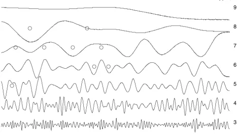
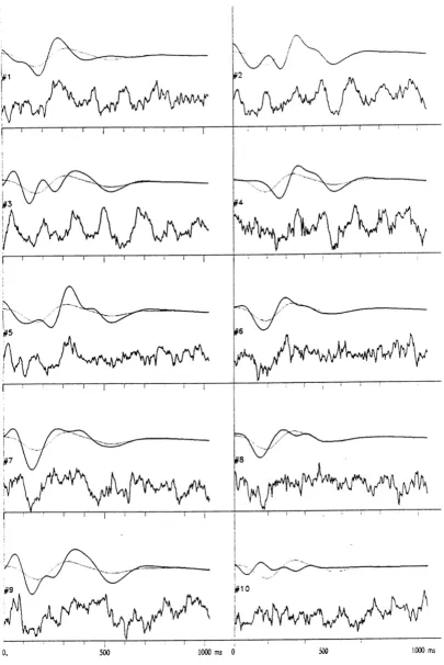
First successful applications of wavelets addressed the is-sue of evoked potentials (EP). Event-related potentials are small changes of EEG activity in response to an external (evoked) or internal stimulus. They are usually an order of magnitude weaker than the on-going EEG activity, so tra-ditionally they were observed only in time averages of stimulus-synchronized repetitions. Owing to the property of the time synchronization, they can be studied in the space of orthogonal wavelet coefficients. Figures 2,3,4 present the first wavelet study of evoked potentials [5]. Randomly chosen epochs of on-going EEG were statisti-cally compared – in the space of wavelet coefficients – to those synchronized by an auditory stimulus. As a result, only 9 out of 512 coefficients were found to discriminate between those conditions. They were enough to repro-duce the basic morphology of the average EP. Figure 4 presents reconstruction of single evoked potentials using those coefficients.

Limitations of linear and quadratic time-frequency representations

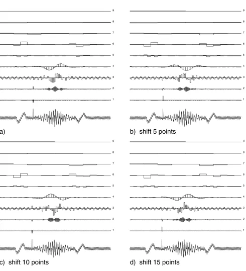
Further attempts to apply wavelets to the analysis of on-going EEG activity encountered a major drawback. Repre-sentation of the signal, obtained from orthogonal wavelet representation, is not time-shift invariant. This property is illustrated in Figure 5.

This limitation is not present in the continuous wavelet transform, as well as several quadratic representations of signal's energy density in the time-frequency plane (c.f. [6] and Figure 8). However, in such case we loose the compact description offered by orthogonal wavelets – the

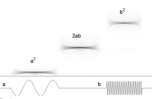
representation is highly redundant. Another problem re-lates to the occurence of cross terms (Figure 6).

Both these problems can be solved (or at least significant-ly reduced) by the solution proposed in the next section.

Adaptive approximations and matching pursuit

Given a set of functions (dictionary) D = {g₁,g₂...g_n} such that ||g_i|| = 1, we can define an optimal M-approximation as an expansion, minimizing the error ε of an approxima-tion of signal f(t) by M waveforms:

where {γ_i}_{i = 1..M} represents the indices of the chosen functions gγi. Finding such an optimal approximation is an NP-hard problem. A suboptimal expansion can be found by means of an iterative procedure, such as the matching pursuit algorithm (MP) proposed by Mallat and Zhang [7].

In the first step of MP, the waveform g_γ0 which best match-es the signal f(t) is chosen. In each of the consecutive steps, the waveform gγn is matched to the signal Rn_{f, which}

is the residual left after subtracting results of previous iterations:

Orthogonality of Rn+1 _{f and gγn in each step implies energy}

conservation:

For a complete dictionary the procedure converges to f:

From this equation we can derive a time-frequency distri-bution of the signal's energy, that is free of cross-terms, by adding Wigner distributions of selected functions:

ε=

( )

( )

( )

=

∑

f t _ig t

i M

i 1

1

R f f

R f R f g g R f

g R f g

n n n

g D n

n n

n i i

0

1

=

=< > +

= < >

       + ∈ ,

arg max ,

γ γ

γ γ γ

2 2

( )

f R f gn R fm

n m

n

2 2 2

0 1

3

= < > +

( )

= −

∑

f R f gn g

n n n

= < >

( )

= ∞

∑

0

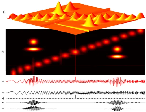
This magnitude is presented in Figure 7, calculated from MP decomposition of a simulated signal with known and simple content. We observe that most of the structures are represented compactly and with high resolution, except for the structure of changing frequency (linear chirp). It is represented by a series of structures of constant frequency, since in the applied Gabor dictionary (section 5) we have only constant frequency modulations. Section 7 presents an alternative approach to this issue.

Figure 8 presents estimates of the time-frequency density of the same signal's energy, obtained from: spectrograms

with different window widths, continuous wavelet trans-form and smoothed pseudo Wigner-Ville distribution. Only in the last case representation of the chirp looks bet-ter than on the plot obtained from MP decomposition, but we must take into account that in this case the param-eters of the kernel of the distribution were optimized for this particular signal.

Except for the lack of cross terms and high resolution, adaptive time-frequency parametrizations exhibit one more basic and important advantage over the continuous time-frequency representations. Unlike the maps from Figure 8, for all the structures presented in Figure 7 we have a priori the exact values of their time and frequency centers, widths, amplitudes and phases. This property will be thoroughly explored in the following studies.

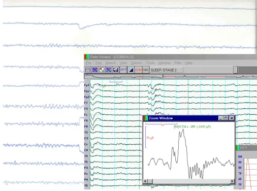
Figure 1

70 years of progress in clinical EEG analysis: from visual analysis of EEG traces on paper (background picture) to visual analysis of EEG traces displayed on CRT (front). From [4].

Ef t R f gn Wg t

n M

n n

,ω , _{γ γ} ,ω

( )

( )

( )

=

∑

0

Figure 2

Average auditory evoked potential, it's decomposition in wavelet subbands and reconstruction from 9 wavelet coefficients, sta-tistically differentiating EP from on-going EEG ([5]).

1

2

3

4

5

6

7

8

9

epp.avr, ch. 0

Figure 3

Single AEP, reconstructed as in Figure 2

1

2

3

4

5

6

7

8

9

epp.9, ch. 0

Figure 4

Figure 5

Orthogonal wavelet representation is not time-shift invariant: wavelet decomposition of simulated signal shifted in time. Heights of rectangles at each level proportional to the value of wavelet coefficients at given scale.

a)

P.J. Durka IFD UW: FALKI

1 2 3 4 5 6 7 8 9

b) shift 5 points

P.J. Durka IFD UW: FALKI

1 2 3 4 5 6 7 8 9

c) shift 10 points

1 2 3 4 5 6 7 8 9

d) shift 15 points

First application in EEG analysis: sleep spindles

The presence of sleep spindle should not be defined un-less it is of at least 0.5 sec duration, i.e., one should be able to count 6 or 7 distinct waves within the half-second period. (...) The term should be used only to describe ac-tivity between 12 and 14 cps.

– says the definition from the basic reference [8] – "A manual of standardized terminology, techniques and scoring system for sleep stages in human subjects". It can be directly translated into the language of parameters of the structures fitted to the signal by the algorithm dis-cussed in the previous section.

By choosing from the time-frequency atoms, fitted to EEG by the MP algorithm, those conforming to the above cri-teria, we obtain a detailed, automatic and high-resolution parametrization of the relevant structures, which corre-spond to sleep spindles [9,10]. Figures 10 and 11 present

results of such a procedure carried out for several deriva-tions of an overnight sleep EEG recording. This parametri-zation has proven to be consistent with visual detection, especially for the structures of higher amplitudes [11]. For lower amplitudes the algorithm detects also spindles elu-sive to a human expert.

Results presented in these figures conform also the previ-ously observed effect of predominance of lower frequen-cies of sleep spindles in frontal derivations and higher frequencies in parietal derivations. We also notice that some frequencies on these plots are "prefereed", i.e. ex-hibit regular maxima in the histograms. But are they pre-ferred by the brain or by the analysis algorithm? This question will be resolved in the next section.

Figure 6

Cross-terms in time-frequency representations of signal's energy: (a + b)2 _{= a}2 _{+ b}2 _{+ 2ab. Wigner-De Ville transform (above)}

Discrete Gabor dictionary

Gabor functions (sine-modulated Gaussian functions) provide optimal joint time-frequency localization. A real Gabor function can be expressed as:

N is the size of the signal for which the dictionary is con-structed, K(γ) is such that ||gγ|| = 1. γ = {u,ω,s,φ } denotes

parameters of the dictionary's functions (time-frequency atoms). These parameters generate a three-dimensional continuous space; this results in an infinite dictionary size. Therefore, in practical implementations, we use sub-sets of the possible dictionary's functions.

In the dictionary implemented originally by Mallat and Zhang in [7], parameters of these functions (time-fre-quency atoms) are chosen from dyadic sequences of inte-gers. Their sampling is governed by an extra parameter – octave j (integer). Scale s, which corresponds to an atom's Figure 7

Time-frequency map of energy density of a 500-points simulated signal (e) composed of four sine-modulated Gaussians, i.e. Gabor functions (a-b), sine wave and one-point discontinuity (c) and sine wave with linear frequency modulation-chirp (d). Dis-tribution (f) was obtained from a decomposition in a large (2 * 106 _{waveforms) dictionary. Changing frequency of the chirp is}

represented as a series of functions, since in the Gabor dictionary (section 5) we have only constant frequency modulations, (g)-the same as (f), presented in 3 dimensions. Square root of energy proportional to the height of the surface or "tempera-ture" on 2-dimensional plots. [22]

g t K e

N t u t u

s

γ

π

γ π ω φ

( )= ( )  ( − )+ 



 ( )

−  − 

 

2

2 6

Figure 8

width in time, is derived from the dyadic sequence s = 2j_,

0 ≤ j ≤ L (signal size N = 2L_{). Parameters u and ω, which}

correspond to position in time and frequency, are sam-pled for each octave j with interval s = 2j_{, or, if}

oversam-pling by l is introduced, with interval 2j-l_.

This specific wavelet-like structure of the dictionary is re-sponsible for the fact that decomposition over such a dic-tionary "prefers" certain positions in frequency or time (Figures 12, 13). In those positions more atoms are avail-able for decomposition due to the particular structure of the dictionary, i.e. scheme of subsampling the parameter space.

Stochastic dictionaries

In forming the dictionary used for MP decomposition, us-ing any fixed scheme of subsamplus-ing the parameter space introduces statistical bias in the resulting parametrization. This bias becomes apparent only when statistics comes into play, like in parameterization of large amounts of da-ta. Unbiased MP decompositions can be obtained by an analogue of Monte Carlo methods.

In [12] we proposed MP with stochastic dictionaries, where the parameters of a dictionary's atoms are rand-omized before each decomposition. A stochastic diction-ary D is constructed for a given signal length N and chosen "resolutions"1 _{in time, frequency and scale (∆t, ∆ω and}

∆s). The space of parameters t, ω and s is thereby divided

into bricks of size ∆t by ∆ω by ∆s each, where ω ∈ (0,π). In each of those bricks, one time-frequency atom is chosen by drawing its parameters from flat distributions within the given ranges of continuous parameters.

Figures 14 and 15 present results for the same data as Fig-ures 10 and 11. These results, owing to the application of the above described stochastic dictionaries, are free from the statistical bias.

1_{The resolution of the matching pursuit is hard to define}

in general, since the procedure is nonlinear and signal-de-pendent. It should be related to the distance between neighboring dictionary waveforms available for Figure 9

Time-frequency energy distribution (equation 5) of 20 seconds of sleep EEG; structures corresponding to sleep spindles are marked by letters A-F. Structures C and D, as well as E and F, were classified as one spindle, i.e. their centers fell within a time section marked by expert as one spindle's occurrence. [23]

F

F

E

E

A

A

B

B

D

D

C

C

2

4

6

8

10

12

14

16

18

20 Hz

0 2.5 5 7.5 10 12.5 15 17.5 20 s

1 s

∏ ∆ ∆ ∆ω

N t s

Figure 10

Histograms of frequencies of sleep spindles detected in one overnight EEG recording. Plots are placed on page according to relative positions of corresponding derivations from the 10–20 system – front of head towards the top of page

Fp1

10.0 12.0 14.0 [Hz] 0

100 200

No Fpz

10.0 12.0 14.0 [Hz] 0

100 200

No Fp2

10.0 12.0 14.0 [Hz] 0

100 200 No

F7

10.0 12.0 14.0 [Hz] 0

100 200

No F3

10.0 12.0 14.0 [Hz] 0

100 200

No Fz

10.0 12.0 14.0 [Hz] 0

100 200

No F4

10.0 12.0 14.0 [Hz] 0

100 200

No F8

10.0 12.0 14.0 [Hz] 0

100 200 No

T3

10.0 12.0 14.0 [Hz] 0

100 200

No C3

10.0 12.0 14.0 [Hz] 0

100 200

No Cz

10.0 12.0 14.0 [Hz] 0

100 200

No C4

10.0 12.0 14.0 [Hz] 0

100 200

No T4

10.0 12.0 14.0 [Hz] 0

100 200 No

T5

10.0 12.0 14.0 [Hz] 0

100 200

No P3

10.0 12.0 14.0 [Hz] 0

100 200

No Pz

10.0 12.0 14.0 [Hz] 0

100 200

No P4

10.0 12.0 14.0 [Hz] 0

100 200

No T6

10.0 12.0 14.0 [Hz] 0

100 200 No

O1

10.0 12.0 14.0 [Hz] 0

100 200

No Oz

10.0 12.0 14.0 [Hz] 0

100 200

No O2

10.0 12.0 14.0 [Hz] 0

Figure 11

Amplitudes of detected spindles (vertical) plotted versus their frequencies (horizontal) for the same data and derivations as Fig 10

F3

10.0 12.0 14.0 [Hz]

25 45 65

[microV] Fz

10.0 12.0 14.0 [Hz]

25 45 65

[microV] F4

10.0 12.0 14.0 [Hz]

25 45 65

[microV]

C3

10.0 12.0 14.0 [Hz]

25 45 65

[microV] Cz

10.0 12.0 14.0 [Hz]

25 45 65

[microV] C4

10.0 12.0 14.0 [Hz]

25 45 65

[microV]

P3

10.0 12.0 14.0 [Hz]

25 45 65

[microV] Pz

10.0 12.0 14.0 [Hz]

25 45 65

[microV] P4

10.0 12.0 14.0 [Hz]

25 45 65

decomposition. In the described procedure, this distance does not exceed twice the value of the corresponding pa-rameter (∆t, ∆ω or ∆s).

Pharmaco EEG

This section presents an application of the proposed methodology to the standard clinical problem of testing influence of sleep inducing drugs on the sleep EEG.

The effects of zolpidem, midazolam and placebo, admin-istered at bed time, were studied in 7 paid volunteers. From each of the 21 all-night recordings (3 nights for each subject) we extracted artifact-free epochs from derivation

C3-A2 of the 10–20 system. For the analysis of slow wave activity (SWA) we used data from stages III and IV and for sleep spindles only data from sleep stage II.

Figures 16 and 18 present the classical approach to the analysis of these data, that is averaging the spectral inte-grals in the above mentioned ranges, for each of the ana-lyzed recordings.

Figures 17 and 19 present each of the structures, classified as sleep spindles (Figure 17) or SWA (Figure 19) as a dot in the frequency-amplitude plane. These structures were selected using not only the frequency information, as in Figure 12

200 realizations of 128-points white noise process were subjected to MP decomposition in dyadic (middle plot) and stochastic (bottom) dictionaries. The middle and lower plots present histograms of frequencies of all the structures fitted by MP. The upper plot is a histogram of frequencies of all the time-frequency atoms present in the dyadic dictionary used for the decompo-sition presented in the middle plot.

histograms of frequencies:

_{dyadic dictionary}

0

1000

2000

all structures from dyadic MP decomposition of noise

0

200

400

600

0

π

/4

π

/2

3

π

/4

Figure 13

Statistical properties of MP decomposition of 50 epochs of sleep EEG (a, b) and white noise (c-f) over dyadic (a, c, e) and sto-chastic (b, d, f) dictionaries. Histograms of frequency centers of atoms fitted by MP decomposition over dyadic dictionary to EEG (a) and noise (c) reveal additional structure, absent in corresponding decompositions performed over stochastic diction-aries b and d, respectively. Maximum in the middle of frequency range in panel d results from convention of assigning half of Nyquist frequency to Dirac's delta. In the top panel centers of atoms fitted to white noise are given in the time-frequency plane for dyadic (left, e) and stochastic (right, f) dictionaries

(d)

0.0 0.1 0.2 0.3 0.4

0 100 200

No

(c)

0.0 0.1 0.2 0.3 0.4

0 100 200

No

(b)

0.0 10.0 20.0 30.0 40.0 50.0 60.0 [Hz

0 100 200

No

(a)

0.0 10.0 20.0 30.0 40.0 50.0 60.0 [Hz]

0 100 200

No

(e)

0.0 100.0 200.0 300.0 400.0 500.0

0.00 0.10 0.20 0.30 0.40

(f)

0.0 100.0 200.0 300.0 400.0 500.0

Figure 14

Histograms of frequencies of sleep spindles detected in the same EEG recording as in Figure 10, decomposed in stochastic dictionaries

F3

10.0 12.0 14.0 [Hz]

0 100 200

No Fz

10.0 12.0 14.0 [Hz]

0 100 200

No F4

10.0 12.0 14.0 [Hz]

0 100 200

No

C3

10.0 12.0 14.0 [Hz]

0 100 200

No Cz

10.0 12.0 14.0 [Hz]

0 100 200

No C4

10.0 12.0 14.0 [Hz]

0 100 200

No

P3

10.0 12.0 14.0 [Hz]

0 100 200

No Pz

10.0 12.0 14.0 [Hz]

0 100 200

No P4

10.0 12.0 14.0 [Hz]

0 100 200

Figure 15

Amplitudes of sleep spindles (vertical) plotted versus their frequencies (horizontal) detected in the same EEG recording as in Figure 11 (as well as 10 and 14), based upon MP decomposition with stochastic dictionaries

F3

10.0 12.0 14.0 [Hz]

25 45 65

[microV] Fz

10.0 12.0 14.0 [Hz]

25 45 65

[microV] F4

10.0 12.0 14.0 [Hz]

25 45 65

[microV]

C3

10.0 12.0 14.0 [Hz]

25 45 65

[microV] Cz

10.0 12.0 14.0 [Hz]

25 45 65

[microV] C4

10.0 12.0 14.0 [Hz]

25 45 65

[microV]

P3

10.0 12.0 14.0 [Hz]

25 45 65

[microV] Pz

10.0 12.0 14.0 [Hz]

25 45 65

[microV] P4

10.0 12.0 14.0 [Hz]

25 45 65

Figure 16

Spectral estimates of power in the frequency range of sleep spindles. Columns correspond to results for the night after admin-istrating, from left to right: placebo, zolpidem, midazolam. Each row contains results for one subject. Plots present average (in stage II) spectrum between 12 and 14 Hz. Numbers on the right of each plot, from the top: % change of power related to the night after administrating placebo (absent in the first column), value of the total power between 12 and 14 Hz (µV2_{), it's mean}

square error (mse) and total time of stage II (in minutes) for given recording. We observe general trend of increase of power in this band, except for one case – the last subject, night after midazolam (bottom right)

ZCB02C

4.07 µV2

mse=0.11

204.1 min.

ZCB02B

+51%

6.14 µV2

mse=0.18

147.7 min.

ZCB02A

+40%

5.69 µV2

mse=0.16

241.5 min.

ZCB03B

8.41 µV2

mse=0.30

107.5 min.

ZCB03C

+19%

10.02 µV2

mse=0.32

90.5 min.

ZCB03A

+35%

11.38 µV2

mse=0.31

158.3 min.

ZCB04C

6.83 µV2

mse=0.23

107.5 min.

ZCB04A

+8%

7.38 µV2

mse=0.23

132.1 min.

ZCB04B

+33%

9.07 µV2

mse=0.35

76.5 min.

ZCB06B

5.12 µV2

mse=0.12

239.9 min.

ZCB06A

+27%

6.49 µV2

mse=0.18

184.7 min.

ZCB06C

+87%

9.58 µV2

mse=0.22

260.4 min.

ZCB07A

10.66 µV2

mse=0.30

171.7 min.

ZCB07B

+9%

11.64 µV2

mse=0.48

95.3 min.

ZCB07C

+12%

11.94 µV2

mse=0.42

150.5 min.

ZCB08B

8.53 µV2

mse=0.23

108.7 min.

ZCB08A

+22%

10.40 µV2

mse=0.25

158.7 min.

ZCB08C

+43%

12.17 µV2

mse=0.31

122.4 min.

ZCB09A

2.42 µV2

mse=0.06

110.8 min.

ZCB09C

+18%

2.85 µV2

mse=0.06

211.9 min.

st:0010000, 12.00−14.00 Hz, 20−Aug−2001

12 13 14 0 0.5 1 1.5 ZCB09B −4%

2.33 µV2

mse=0.07

Figure 17

Sleep spindles selected from the MP parametrization of the same recordings as in Figure 16 – plots organized accordingly – chosen as structures with frequency 12–14 Hz, amplitude above 15 µV and time duration 0.5–2.5 seconds. Each dot in the plots marks one spindle in the frequency (horizontal, Hz) versus amplitude (vertical, µV) coordinates. Numbers on the right of each plot give increase of total power relative to the night after placebo (absent in first column), power carried by selected struc-tures, number of structures per minute (in parenthesis total time of qualified stages in min.), average amplitude and its variance, and average (weighted by amplitude) frequency with variance

1.5 /min (204) 0.8 µV2

13.36 Hz v0.5 21.6 µV v6.2 ZCB02C

+118%

2.8 /min (148) 1.8 µV2

13.46 Hz v0.5 22.4 µV v7.2 ZCB02B

+132%

2.9 /min (242) 1.9 µV2

13.36 Hz v0.5 22.7 µV v7.4 ZCB02A

4.2 /min (107) 2.9 µV2

13.12 Hz v0.6 23.2 µV v7.1 ZCB03B

+35%

5.2 /min (91) 3.9 µV2

13.22 Hz v0.5 23.3 µV v6.7 ZCB03C

+58%

5.6 /min (158) 4.5 µV2

13.25 Hz v0.5 24.1 µV v7.5 ZCB03A

2.7 /min (107) 1.7 µV2

13.22 Hz v0.6 23.1 µV v7.5 ZCB04C

+16%

3.1 /min (132) 2.0 µV2

13.22 Hz v0.7 23.0 µV v7.2 ZCB04A

+76%

4.2 /min (76) 3.0 µV2

13.19 Hz v0.5 23.8 µV v8.4 ZCB04B

2.0 /min (240) 1.2 µV2

13.41 Hz v0.6 22.6 µV v6.9 ZCB06B

+94%

3.6 /min (185) 2.3 µV2

13.38 Hz v0.5 22.9 µV v6.9 ZCB06A

+242%

5.0 /min (261) 4.1 µV2

13.28 Hz v0.4 24.3 µV v8.1 ZCB06C

4.5 /min (172) 3.6 µV2

13.06 Hz v0.5 25.4 µV v9.4 ZCB07A

+45%

5.8 /min (95) 5.2 µV2

13.02 Hz v0.5 26.5 µV v9.8 ZCB07B

+54%

5.8 /min (151) 5.5 µV2

12.82 Hz v0.5 26.9 µV v11.2 ZCB07C

3.1 /min (109) 1.9 _µV2

13.03 Hz v0.6 23.0 µV v7.2 ZCB08B

+49%

4.2 /min (159) 2.9 _µV2

13.16 Hz v0.6 23.5 µV v8.4 ZCB08A

+76%

4.9 /min (122) 3.4 _µV2

13.12 Hz v0.6 23.9 µV v8.3 ZCB08C

0.4 /min (111) 0.2 _µV2

13.53 Hz v0.4 19.4 µV v4.1 ZCB09A

amp/frq, st:0010000, 12.00−14.00 Hz, a:15−Inf µV, w:0.5−2.5 s. 28−Aug−2001

+148%

1.0 /min (212) 0.4 _µV2

13.47 Hz v0.4 20.0 µV v4.2 ZCB09C

+84%

0.7 /min (127) 0.3 _µV2

13.49 Hz v0.4 20.4 µV v4.7

12 13 14 0

20 40 60

Figure 18

Spectral (FFT-based) estimates of power of slow wave activity (SWA) in the 0.75–4 Hz frequency range, plots and description organized as in Figure 16

ZCB02C

960.33 µV2

mse=33.79

75.3 min.

ZCB02B

−34%

637.61 µV2

mse=16.97

126.6 min.

ZCB02A

−37%

601.03 µV2

mse=20.00

104.3 min.

ZCB03B

652.37 µV2

mse=17.01

98.7 min.

ZCB03C

−5%

618.80 µV2

mse=16.32

84.5 min.

ZCB03A

−16%

548.15 µV2

mse=15.86

78.9 min.

ZCB04C

911.54 µV2

mse=20.35

137.1 min.

ZCB04A

−21%

719.53 µV2

mse=16.34

121.6 min.

ZCB04B

−7%

850.67 µV2

mse=24.73

62.4 min.

ZCB06B

897.11 µV2

mse=26.34

96.6 min.

ZCB06A

−31%

615.04 µV2

mse=16.59

134.5 min.

ZCB06C

−25%

675.22 µV2

mse=22.28

99.7 min.

ZCB07A

847.35 µV2

mse=39.41

42.3 min.

ZCB07B

−4%

816.65 µV2

mse=46.59

34.4 min.

ZCB07C

−25%

633.66 µV2

mse=38.93

29.7 min.

ZCB08B

383.77 µV2

mse=13.55

58.1 min.

ZCB08A

−8%

352.96 µV2

mse=10.17

64.3 min.

ZCB08C

+10%

422.33 µV2

mse=11.73

67.3 min.

ZCB09A

324.43 µV2

mse=10.57

77.5 min.

ZCB09C

−10%

291.56 µV2

mse=9.60

65.5 min.

st:1100000, 0.75−4.00 Hz, 20−Aug−2001 1 2 3 4 0 100 200 300 ZCB09B −33%

218.77 µV2

mse=5.21

Figure 19

Slow wave activity (SWA) selected from the MP parametrization as structures of frequency 0.75–4 Hz, amplitude higher than 75 µV and duration above half a second. Plots and descriptions organized as in Figure 17

9.9 /min (75) 443.9 µV2

1.18 Hz v0.5 131.7 µV v66.6 ZCB02C

−52%

6.6 /min (127) 214.5 µV2

1.17 Hz v0.5 117.9 µV v51.1 ZCB02B

−62%

5.0 /min (104) 169.5 µV2

1.13 Hz v0.5 120.1 µV v51.5 ZCB02A

6.5 /min (99) 180.4 µV2

1.19 Hz v0.5 114.4 µV v43.4 ZCB03B

−24%

5.3 /min (84) 137.8 µV2

1.12 Hz v0.4 110.2 µV v37.5 ZCB03C

−30%

4.9 /min (79) 126.0 µV2

1.10 Hz v0.4 112.8 µV v42.0 ZCB03A

11.6 /min (137) 415.4 µV2

1.28 Hz v0.5 123.7 µV v50.5 ZCB04C

−29%

9.2 /min (122) 292.9 µV2

1.24 Hz v0.5 124.3 µV v52.8 ZCB04A

−12%

10.9 /min (62) 365.5 µV2

1.24 Hz v0.5 118.3 µV v46.1 ZCB04B

10.0 /min (97) 396.5 µV2

1.26 Hz v0.5 131.2 µV v64.4 ZCB06B

−57%

5.9 /min (134) 168.7 µV2

1.18 Hz v0.5 115.8 µV v54.2 ZCB06A

−44%

6.5 /min (100) 220.2 µV2

1.19 Hz v0.5 123.0 µV v55.9 ZCB06C

9.7 /min (42) 371.6 µV2

1.28 Hz v0.6 131.7 µV v60.8 ZCB07A

−34%

7.1 /min (34) 244.4 µV2

1.27 Hz v0.5 124.0 µV v50.9 ZCB07B

−44%

6.1 /min (30) 209.4 µV2

1.14 Hz v0.5 123.8 µV v56.0 ZCB07C

4.8 /min (58) 107.7 µV2

1.19 Hz v0.5 108.8 µV v34.6 ZCB08B

−40%

3.6 /min (64) 64.7 µV2

1.13 Hz v0.4 101.3 µV v29.0 ZCB08A

−13%

4.4 /min (67) 93.4 µV2

1.17 Hz v0.5 107.2 µV v33.3 ZCB08C

3.7 /min (77) 87.0 µV2

1.12 Hz v0.5 110.0 µV v37.7 ZCB09A

amp/frq, st:1100000, 0.75−4.00 Hz, a:75−Inf µV, w:0.5−Inf s. 28−Aug−2001

−25%

2.7 /min (65) 64.9 µV2

1.03 Hz v0.4 109.2 µV v35.6 ZCB09C

−64%

1.4 /min (136) 31.2 µV2

0.98 Hz v0.3 106.3 µV v33.4

1 2 3 4 0

200 400

the "classical" approach, but also information on time du-ration and amplitude from Table 1. Total power carried by these structures, summed and normalized per time unit, is indicated on the right of each plot, together with the aver-age number of occurrences per minute, averaver-age amplitude and frequency.

We observe that selective MP-based estimates of power are more sensitive to the effect of influence of both drugs than the spectral integrals. This sensitivity becomes crucial in two of the analyzed cases:

1. In the recording of patient ZCB09, which revealed a very low spindling activity (last row in Figures 16 and 17), fluctuations in the background masked the power of sleep spindles to such an extent, that spectral integrals indicate a partially reverse trend, i.e. decrease of power of sleep spindles under the influence of midazolam. Selective esti-mates indicate the expected increase.

2. For patient ZCB08 (second row from the bottom) spec-tral integrals indicate increase of power of SWA (δ), while MP estimates reveal a decrease coherent with all the other cases.

Finally, as an example of an effect elusive to the classical methodology, these results indicate also a statistically sig-nificant decrease of the frequency of the slow wave activi-ty. Further discussion and statistical evaluation of results can be found in [13].

Figure 20 partially explains the increased sensitivity of the proposed approach as compared to the classical paradigm of band-limited spectral power integrals.

Representation of changing frequency

Another interesting property of the stochastic time-fre-quency dictionaries, discussed in section 5.1, relates to the representation of structures of changing frequency. Such structures are absent in the dictionaries usually applied for

Table 1: Criteria chosen for the automatic selection of EEG structures based upon the time-frequency parameters.

frequency duration amplitude

SWA 0.75–4 Hz 0.5-∞s. >75 µV

sleep spindles 12–14 Hz 0.5–2.5 s. > 15 µV

Figure 20

Distinction between a spectral power integral from f₁ to f₂, and power actually carried by structures of frequencies centered between f₁ and f₂. Plot a) presents spectral power (versus frequency) of hypothetical structures with frequency centers lying inside (dotted) and outside (dashed line) the f₁-f₂ interval. Due to the uncertainty principle, their spectral contents overlap. Solid line presents their sum, i.e. total spectral power, as estimated e.g. by Fourier transform. In b) the actual power carried by structure of frequency originating between f₁ and f₂, as estimated in the proposed approach, is shaded. Plot c) highlights the power obtained from a spectral integral from f₁ to f₂. Finally in d) additional background (dotted-dashed line) is added. We observe that neighboring structures from outside the interval of interest may contribute significantly to the power estimated within the interval, and can even shift the actual position of the spectral peak related to the relevant structure (dotted line), while some of the power carried by the structure inside the interval of interest falls outside and does not contribute to the spectral integral

f

1

f

a)

f

1

f

b)

f

1

f

c)

f

1

f

the decomposition, and therefore are represented as a series od fixed-frequency Gabor functions (Figure 22 (f) and Figure 21 (b)).

However, by averaging several decompositions of the same signal in different realizations of smaller stochastic dictionaries, we obtain a more continuous representation like in Figures 22 (g) and Figure 21 (c). The representation is no more compact, but retains the general property of absence of cross terms.

Event-related desynchronization and

synchronization

Advantages of the MP algorithm with stochastic dictionar-ies can be also combined with the stochastic element present inherently in the data, like e.g. in the case of analyzing repetitions of event-related potentials. This re-lates especially to the non-phase locked activity, i.e. such that would not be enhanced in the stimulus-synchronized time averages. Its detection requires a different analysis technique, allowing for averaging signal's energy irrelevant of the phase2_{. Classically it was achieved by}

squaring the values of signals, band-pass filtered in a priori chosen frequency bands, before averaging ([14], Figure 23).

Figure 21

Figure 22

Time-frequency maps of energy density of a 500-points simulated signal (e), the same as in Figure 7, composed of four sine-modulated Gaussians, i.e. Gabor functions (a-b), sine wave and one-point discontinuity (c) and sine wave with linear frequency modulation-chirp (d). Distribution (f) was obtained from a single decomposition in a large (2 * 106 _{waveforms) dictionary: signal}

is described by only 30 functions, but changing frequency of the chirp is represented as a series of functions, since in the Gabor dictionary we have only constant frequency modulations. (g) presents average of 100 decompositions of the same signal in dif-ferent realizations of smaller (5 * 104 _{atoms) stochastic dictionaries. This smoothes the representation of the chirp, but}

This methodology has several drawbacks, including tha arbitrary choice of frequency bands and limited sensitivity (c.f. Figure 20). Averaging the time-frequency densities of energy, obtained from the MP decomposition, allows for an instantaneous evaluation of the complete picture of changes in the time-frequency plane, with high resolu-tion. Figure 25 presents this picture for the same data as in Figure 23. Another study in Figure 26 reveals clearly split-ting of the alpha band in the upper and lower frequencies, with different behaviour related to the finger movement. This phenomenon would be very difficult to find using the classical methodology.

2_{If we want to analyze phasic synchronization in higher}

frequencies, like e.g. gamma band around 40 Hz, the ac-curacy of the triger's determination would have to be much better than e.g. 1 ms, which is rather beyond the accuracy of determining e.g. the moment of a finger movement. But non-phasic effects should be visible in the presented approach.

Epileptic seizures

Discussed advantages of time-frequency estimates of ener-gy density, obtained from MP decomposition, allowed for identification of different dynamic states during evolution and propagation of epileptic seizures in [15].

Figure 27 presents an example of time-frequency density of energy, calculated from the MP expansion of an intracranial recording of epileptic seizure. Sensitivity of the algorithm to the phase changes clearly distinguishes the initial less synchronized period of transitional rhytmic activity (starting near 15th second) from the organized rhytmic activity. In this period (starting about 30th Figure 23

Classical quantification of ERD/ERS in three bands: α 10–12 Hz, (β 14–18 Hz, γ 36–40 Hz. Insert indicates positions of electrodes used for recording. C3, Cz and C4 from the 10– 20 system are marked by thicker circles. Results presented for electrode marked by filled circle [22].

Figure 24

Average time-frequency maps of EEG energy density, obtained from the same data as in Figure 23. Horizontal axis-time in seconds relative to the finger movement. Vertical axes on the right of those maps indicate frequency in Hz. Energy proportional to shades of gray. Scale is arbitrary and different for each map. Curves above the maps, correspond-ing to figure 3, are frequency integrals of the maps below them. Vertical axes on their left sides indicate percent of change, relative to energy integrated between 3.5 and 4.5 seconds before the movement in given band. [22]

36 38 40 0

2009

14 16 18 −83

0 137

−4 −3 −2 −1 0 1 2 3 4 10 12 −90

second) all the harmonics, up to the Nyquist frequency, clearly follow the pattern of decreasing frequency. Such a clear representation of changing frequency was possible using the technique discussed in section 7.

Problems

As presented in figure 28, greedy MP algorithm in certain cases can fail to properly decompose signal containing even a simple combination of dictionary's functions. This counterexample was simulated especially for discussion of practical issues and as such may look scary, but on the other hand we never encountered such a failure in applications to real world signals. The trap in this case lies

in the fact that both these structures have exactly the same phase, and it might be even dicussable if they should not be treated as one in the first approximation. If they were produced by two different biological generators, such a coincidence of phases would not be possible and they would be parametrized separately.

Other, more theoretical examples of MP failures are given in [16] and [17]. Some of these cases can be properly solved by the orthogonalized matching pursuit [18], at a cost of increased computational requirements and a possibility of introducing numerical instabilities [19]. An-other modification of the MP algorithm, discussed in Figure 25

Figure 26

[20], relies on a modification of the similarity function used in each step to choosed the "best fit". Other works [21] indicate that global optimalization of the l1 _{norm of}

expansion's coefficients might be the best choice [17], but, in spite of recent advances in linear programming, computational complexity is still very high.

Other problems, awaiting better solutions, include: effi-cient and (at the same time) bias-free implementations, robust estimation of resolution, proper addressing of the tradeoff between resolution (increasing dictionary size) and computation cost, and extension of the algorithm to

the multichannel case. Such research will improve effectivity and understanding of mathematical founda-tions of these higly nonlinear procedures. However, cur-rent implementations and knowledge of algorithm's properties are already sufficient for large scale applica-tions in EEG research and clinical practice. They may serve as a basis for a unification of parametrization and descrip-tion of EEG.

Implementations of MP with stochastic dictionaries is available from http://brain.fuw.edu.pl/mp.

Figure 27

Bottom: intracranial recording of an epileptic seizure, horizontal axis in seconds, sampling 100 Hz. Middle time-frequency dis-tribution of energy was obtained as average of 17 MP decompositions in different realizations of a stochastic dictionary (3 * 106

Authors contributions

Parts of presented research, according to the quoted refer-ences, were coauthored by:

• Prof. Katarzyna J. Blinowska, head of the Laboratory of Medical Physics, Warsaw University, and my colleagues from the Lab: Józef Ginter Jr, Dobiesaw Ircha, Jarosaw Zygierewicz.

• Prof. Waldemar Szelenberger, Medical University of Warsaw

• Prof Ernest A. Bartnik, Inst. of Theoretical Physics, War-saw University

• Prof. Piotr Franaszczuk, Johns Hopkins Medical University

• Prof. Gert Pfurtscheller and dr Christa Neuper, Graz Technical University

References

1. Hans Berger Über das elektrenkephalogramm des menschen.

Arch f Psychiat 1929, 87:527-570

2. Ernst Niedermayer and Lopes Da Silva F Electroencephalography: Basic Principles, Clinical Applications and Related Fields. Wil-liams & Wilkins 1999, 1154

3. Dietsch G Fourier Analyse von Elektroenzephalogrammen des Menschen.Pflügers Arch Ges Physiol 1932, 230:106-112 4. Durka PJ and Blinowska KJ A unified time-frequency

parametri-zation of EEG.IEEE Engineering in Medicine and Biology Magazine

2001, 20(5):47-53

5. Bartnik EA, Blinowska KJ and Durka PJ Single evoked potential re-construction by means of wavelet transform.Biol Cybern 1992,

67:175-181

6. Metin Akay and editor Time Frequency and Wavelets in Bio-medical Signal Processing. IEEE Press Series in Biomedical EngineeringIEEE Press 1997,

7. Stéphane Mallat and Zhifeng Zhang Matching pursuit with time-frequency dictionaries.IEEE Transactions on Signal Processing 1993,

41:3397-3415

8. Rechtschaffen A, Kales A and editors A manual of standardized terminology, techniques and scoring system for sleep stages in human subjects.Number 204 in National Institutes of Health Publi-cations. US Government Printing Office, Washington DC 1968, 9. Blinowska KJ and Durka PJ The application of Wavelet

Trans-form and Matching Pursuit to the time-varying EEG signals.

In, Intelligent Engineering Systems through Artificial Neural Networks (Edit-ed by: Dagli CH, Fernandez BR) ASME Press, New York 1994, 4:535-540 10. Durka PJ and Blinowska KJ Analysis of EEG transients by means

of matching pursuit.Ann Biomed Eng 1995, 23:608-611

11. ygierewicz J, Blinowska KJ, Durka PJ, Szelenberger W, Niemcewicz Sz and Androsiuk W High resolution study of sleep spindles.Clin Neurophysiol 1999, 110(12):2136-2147

12. Piotr Durka J, Ircha D and Blinowska KJ Stochastic time-frequen-cy dictionaries for matching pursuit.IEEE Tran Signal Process

2001, 49(3):507-510

13. Durka PJ, Szelenberger W, Blinowska KJ, Androsiuk W and Myszka M

Adaptive time-frequency parametrization in pharmaco EEG.Journal of Neuroscience Methods 2002, 117:65-71

14. Pfurtscheller G and Lopes da Silva FH Event-related EEG/MEG synchronization and desynchronization: Basic principles.Clin Neurophysiol 1999, 110:1842-1857

15. Franaszczuk PJ, Bergey GK, Durka PJ and Eisenberg HM Time-fre-quency analysis using the Matching Pursuit algorithm applied to seizures originating from the mesial temporal lobe.Electroencephalogr Clin Neurophysiol 1998, 106:513-521 16. DeVore RA and Temlyakov VN Some remarks on greedy

algorithms.Advances in Computational Mathematics 1996, 5:173-187 17. Chen SS, Donoho DL and Saunders MA Atomic decomposition

by basis pursuit.SIAM Review 2001, 43(1):129-159

18. Pati YC, Rezaiifar R and Krishnaprasad PS Orthogonal matching pursuit: Recursive function approximation with applications

Figure 28

A failure in feature extraction: MP decomposition of a signal consisting of two Gabor functions, both present in the dictionary used for decomposition. In the left column, from the top: slice of the time-frequency representation obtained from MP decom-position of the signal (R0_{) drawn below; R}1_--R3 _{are first three residues. First three time-frequency atoms (g}

0--g2) fitted by MP

Publish with BioMed Central and every scientist can read your work free of charge "BioMed Central will be the most significant development for disseminating the results of biomedical researc h in our lifetime."

Sir Paul Nurse, Cancer Research UK

Your research papers will be:

available free of charge to the entire biomedical community

peer reviewed and published immediately upon acceptance

cited in PubMed and archived on PubMed Central

yours — you keep the copyright

Submit your manuscript here:

http://www.biomedcentral.com/info/publishing_adv.asp

BioMedcentral

to wavelet decomposition.In Proceedings of the 27th Annual

Asilo-mar Conference on Signals, Systems and Computers November 1993

19. Davis G, Mallat S and Zhang Z Adaptive time-frequency decompositions. SPIE Journal of Optical Engineering 1994,

33(7):2183-2191

20. Jaggi S, Karl WC, Mallat S and Willsky AS High resolution pursuit for feature extraction. 1998,

21. Donoho DL and Huo X Uncertainty principles and ideal atomic decomposition.IEEE Transactions on Information Theory 2001, 47(7):

22. Piotr Durka J, Ircha D, Neuper Ch and Pfurtscheller G Time-fre-quency microstructure of event-related desynchronization and synchronization.Med Biol Eng Comput 2001, 39(3):315-321 23. Piotr Jerzy Durka Time-frequency analyses of EEG.PhD thesis,