Evaluation of the sectional aerosol microphysics module SALSA implementation in ECHAM5-HAM aerosol-climate model

(1)

www.geosci-model-dev.net/5/845/2012/ doi:10.5194/gmd-5-845-2012

Geoscientific

Model Development

Evaluation of the sectional aerosol microphysics module SALSA

implementation in ECHAM5-HAM aerosol-climate model

T. Bergman1,2, V.-M. Kerminen2,3, H. Korhonen1, K. J. Lehtinen1,4, R. Makkonen2, A. Arola1, T. Mielonen1, S. Romakkaniemi4, M. Kulmala2, and H. Kokkola1

1_{Finnish Meteorological Institute, Kuopio Unit, Kuopio, Finland} 2_{University of Helsinki, Department of Physics, Helsinki, Finland} 3_{Finnish Meteorological Institute, Climate Change, Helsinki, Finland}

4_{University of Eastern Finland, Department of Applied Physics, Kuopio, Finland} Correspondence to: T. Bergman ([email protected])

Received: 18 November 2011 – Published in Geosci. Model Dev. Discuss.: 14 December 2011 Revised: 10 May 2012 – Accepted: 12 May 2012 – Published: 18 June 2012

Abstract. We present the implementation and evaluation of

a sectional aerosol microphysics module SALSA within the aerosol-climate model ECHAM5-HAM. This aerosol micro-physics module has been designed to be flexible and compu-tationally efficient so that it can be implemented in regional or global scale models. The computational efficiency has been achieved by minimising the number of variables needed to describe the size and composition distribution. The aerosol size distribution is described using 10 size classes with paral-lel sections which can have different chemical compositions. Thus in total, the module tracks 20 size sections which cover diameters ranging from 3 nm to 10 µm and are divided into three subranges, each with an optimised selection of pro-cesses and compounds.

The implementation of SALSA into ECHAM5-HAM in-cludes the main aerosol processes in the atmosphere: emis-sions, removal, radiative effects, liquid and gas phase sul-phate chemistry, and the aerosol microphysics. The aerosol compounds treated in the module are sulphate, organic car-bon, sea salt, black carcar-bon, and mineral dust. In its default configuration, ECHAM5-HAM treats aerosol size distribu-tion using the modal method. In this implementadistribu-tion, the aerosol processes were converted to be used in a sectional model framework.

The ability of the module to describe the global aerosol properties was evaluated by comparing against (1) measured continental and marine size distributions, (2) observed vari-ability of continental number concentrations, (3) measured sulphate, organic carbon, black carbon and sea-salt mass concentrations, (4) observations of aerosol optical depth

(AOD) and other aerosol optical properties from satellites and AERONET network, (5) global aerosol budgets and con-centrations from previous model studies, and (6) model re-sults using M7, which is the default aerosol microphysics module in ECHAM5-HAM.

The evaluation shows that the global aerosol properties can be reproduced reasonably well using a coarse resolution of 10 sections in size space. The simulated global aerosol bud-gets are within the range of previous studies. Surface con-centrations of sulphate and carbonaceous species have an an-nual mean within a factor of two of the observations. The simulated sea-salt concentrations reproduce the observations within a factor of two, apart from the Southern Ocean over which the concentrations are within a factor of five. Region-ally, AOD is in a relatively good agreement with the observa-tions (within a factor of two). At mid-latitudes the observed AOD is captured well, while at high-latitudes as well as in some polluted and dust regions the modelled AOD is signifi-cantly lower than observed.

(2)

1 Introduction

Aerosols and their interactions with clouds constitute the largest uncertainty in the estimation of present-day radia-tive forcing of the Earth’s atmosphere (Forster et al., 2007; Myhre, 2009; Quaas et al., 2009), hindering seriously our ability to predict the future climate change (Schwartz et al., 2010). Reducing this uncertainty requires detailed informa-tion on the spatial and temporal variability of the concentra-tion, number size distribution and chemical composition of aerosol particles throughout the atmosphere. Necessary tools for getting such detailed information are large-scale mod-elling frameworks together with various measurements plat-forms (Ghan and Schwartz, 2007).

The size-resolved chemical composition of atmospheric aerosols can be simulated in several ways. The most accu-rate and flexible in terms of the shape of the size distribu-tion is the secdistribu-tional method (e.g. Jacobson, 2001; Adams and Seinfeld, 2002; Spracklen et al., 2005); however, it is also computationally the most demanding. In this approach the aerosol population is typically divided into a relatively large number of fixed size bins, and the particle number concen-tration and mass concenconcen-trations of different chemical con-stituents are being tracked separately for each size bin. The second commonly-used method is the modal method that de-scribes the aerosol population with a few log-normal modes (e.g. Binkowski and Roselle, 2003; Vignati et al., 2004; Stier et al., 2005; Sartelet et al., 2006; Pringle et al., 2010; Mann et al., 2010; Zhang et al., 2010). The modal approach is typ-ically much faster than the sectional method, but it has some challenges in accurately describing many climatically im-portant processes, including cloud droplet activation and at-mospheric new-particle formation and growth (Zhang et al., 1999; Sartelet et al., 2006). A more rarely-used approach is the moment method, in which all aerosol processes are tied into different moments of the particle number size distribu-tion (e.g. Bauer et al., 2008). In this method, aerosol prop-erties require an off-line calculation, so this approach can be considered rather inconvenient when interpreting model simulations and comparing the simulations with atmospheric measurements.

Due to computational limitations, most existing large-scale modelling frameworks employ either a modal approach or, alternatively, some combination of modal and sectional or even bulk (only aerosol mass) approaches (e.g. Liu et al., 2005a; Reddy et al., 2005; Liao et al., 2009). The sectional module SALSA (Kokkola et al., 2008) was designed to re-duce the computational burden of traditional sectional mod-els via optimisation of model performance without losing aerosol information relevant to climate simulations. To ob-tain this, the aerosol size distribution is divided into 3 sub-ranges, each with different bin widths and degree of aerosol external mixing. The number of chemical compounds and active processes modelled vary also from one subrange to another. With these simplifications, the number of size bins,

and thus the computational burden, can be reduced signif-icantly without neglecting any of the most significant pro-cesses or chemical compounds. Comparison to a detailed sectional aerosol model demonstrated that SALSA is capa-ble of accurately simulating the basic aerosol microphysical processes in a zero dimensional framework (Kokkola et al., 2008). The main advantage of SALSA compared to modal models is that the sectional method is more flexible in pre-senting the particle size distribution, which can significantly affect, e.g. cloud activation predictions.

In this work, we present an evaluation of the SALSA module in the global general circulation modelling frame-work ECHAM5. We compare the aerosol representation of SALSA to that of the M7 modal model, which is also imple-mented in ECHAM5 (Stier et al., 2005) and which has been applied in several studies (e.g. Lohmann et al., 2007; Hoose et al., 2008; Sesartic et al., 2011; O’Donnell et al., 2011; Par-tanen et al., 2012). Our comparison focuses on global aerosol budgets, aerosol optical properties and particle number size distributions. To assess the qualitative correctness of the rep-resentation, comparisons to in situ measurements and satel-lite observations are performed as well.

2 Model description

2.1 Aerosol-climate model ECHAM5-HAM

The atmospheric general circulation model ECHAM5, de-veloped at Max Planck Institute for Meteorology, is a fifth-generation global climate model (Roeckner et al., 2003, 2004). The prognostic equations are solved as spherical har-monics with triangular truncation. In ECHAM5, the horizon-tal grid is discretised using the spectral transform method. Grid-point calculations are done in a Gaussian grid. For ver-tical discretisation, ECHAM5 uses the hybridσ-pressure co-ordinates with a pressure range from 1013 hPa to 10 hPa. In this study, we have used a spectral truncation of 63 (corre-sponding to approximately 1.9◦×1.9◦on the Gaussian grid) and 31 levels in the vertical. The time step for this resolution is 12 min. Large scale transport uses the Flux Form Semi-Langrangian (FFSL) method by Lin and Rood (1996).

The Hamburg Aerosol Model (HAM) (Stier et al., 2005) handles the emissions, removal and microphysics of aerosol particles within ECHAM5. Emissions and removal processes are partly calculated on-line and partly prescribed. In the ear-lier studies using ECHAM5-HAM, the aerosol microphysics has been calculated using the M7 modal aerosol model by Vignati et al. (2004). In our study we have replaced the M7 model with the SALSA module and compared the differ-ences.

2.2 Nudging

(3)

3 4

4 3

3

3 3

3

2 2

2

2 1

1

1 1

N, SU, OC N, SU, OC, BC, SS, DU

N, SU, OC, BC, DU

N(SS)

N(DU), WS N(DU)

Subregion 1 Subregion 2 Subregion 3

SU – Sulphate OC – Organic carbon BC – Black carbon SS – Sea salt DU – Dust

WS – Water soluble fracCon N() – Number concentraCon only

a

b

c

3 nm 50 nm 700 nm 10 μm

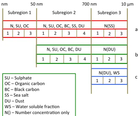
Fig. 1. Schematic of the SALSA sectional structure. There are three parallel sections a, b and c in three subranges each consisting of three or four sections. Parallel size sections in subclass a are soluble, in subclass b insoluble and in subclass c insoluble with possibility for soluble coating enabling cloud activation.

47

Fig. 1. Schematic of the SALSA sectional structure. There are three

parallel sections a, b and c in three subranges, each consisting of three or four sections. Parallel size sections in subclass a are soluble, in subclass b insoluble and in subclass c insoluble, with possibility for soluble coating enabling cloud activation.

relaxes the synoptic scale meteorology towards observed at-mospheric conditions by using atat-mospheric re-analysis data, in our case the ECMWF (The European Centre for Medium-Range Weather Forecasts) operational re-analysis data (Up-pala et al., 2005). While the modelled meteorological fields with nudging are to some extent affected by the model con-figuration (and thus can differ slightly between two model runs due to, e.g. different aerosol forcings), nudging is the best way to quantify the differences in aerosol population that are induced by differences in the aerosol models within the ECHAM5-HAM aerosol-climate model. The simula-tions with both models are performed for the period from July 2007 to December 2008. Spin-up spans the first six months and analysis is done for year 2008.

2.3 SALSA module

The SALSA module describes the aerosol population with a moving center sectional approach (Jacobson, 1997b). SALSA is constructed to allow for flexible modification of the number of sections as well as the locations of the bound-aries between subranges. In the setup used in this study, the size distribution of SALSA consists of 10 size classes with parallel chemical compositions (i.e. some degree of external mixing) and thus simulates 20 sections in total (see Fig. 1). These sections cover diameters ranging from 3 nm to 10 µm and the diameter range is divided into three subranges, each with three or four size sections. The size section boundaries within subranges are spaced logarithmically and shown in Table 1.

Table 1. Particle diameter limits within all sections in SALSA.

Please note that the limits in parallel size bins are the same.

Bin Solubility Minimum Maximum Volume mean diameter diameter diameter

1a1 soluble 3.00 nm 7.7 nm 6.2 nm

2a2 soluble 96.7 nm 187.0 nm 155.0 nm

2a3 soluble 187 nm 362.0 nm 300.0 nm

2a4 soluble 362 nm 700.0 nm 580.1 nm

2b1 insoluble 50.0 nm 96.7 nm 80.1 nm

2b2 insoluble 96.7 nm 187.0 nm 155.0 nm

2b3 insoluble 187.0 nm 362.0 nm 300.0 nm 2b4 insoluble 362.0 nm 700.0 nm 580.1 nm

3a1 soluble 0.70 µm 1.70 µm 1.38 µm

3b1 insoluble 0.70 µm 1.70 µm 1.38 µm

3c1 insoluble 0.70 µm 1.70 µm 1.38 µm

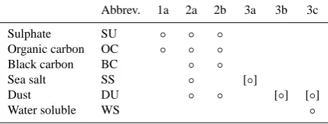
To reduce the computational burden of the module, only the most relevant chemical compounds and microphysical processes are included for each size range. The simulated processes are listed in Table 2 and the compounds in Table 3. Note that in subrange 3c the chemical compounds are not simulated explicitly but lumped into insoluble (i.e. dust) and soluble components. The soluble component includes water soluble compounds (sulphate and organic carbon) transferred from subrange 2b after growth over 700 nm.

The prognostic variables for each section in subranges 1 and 2 are the particle number concentration and the mass concentrations of different chemical components. In the third subrange, the mean diameter is fixed and the only prognos-tic variable in ranges 3a and 3b is number concentration. In subrange 3c, the mass concentration of water soluble (WS) coating on the particles is a prognostic variable.

Subrange 1 consists of three sections and there are no parallel size sections (i.e. no external mixing). This sub-range consists mainly of freshly nucleated particles with a particle diameter between 3 nm and 50 nm. The particle com-pounds include only sulphate and organic carbon.

(4)

Table 2. The processes have been limited to certain size ranges.

Coagulation of large particles is not considered due to low impor-tance. Dry deposition and sedimentation have very limited effect on the population in the smaller soluble size ranges. Nucleation creates new particles only in the smallest size section.

Process 1a 2a 2b 3a 3b 3c

Nucleation ◦

Condensation ◦ ◦ ◦ ◦ ◦ ◦

Coagulation ◦ ◦ ◦

Wet deposition ◦ ◦ ◦ ◦ ◦ ◦

Dry deposition ◦ ◦ ◦ ◦ ◦ ◦

Sedimentation ◦ ◦ ◦ ◦ ◦

all compounds excluding dust, while the insoluble particle sections include all compounds excluding sea salt.

The three size sections in subrange 3 cover the particle size from 700 nm to 10 µm and have three parallel chemi-cal compositions. Most of the particles originate from natu-ral sources. The three externally mixed panatu-rallel compositions sea salt, aged particles from subrange 2 and insoluble dust with water soluble coating. The water soluble compounds sulphate and organic carbon grown from subrange 2b are treated as one compound (water soluble – WS) within the insoluble dust group.

2.4 Microphysical processes

One of the computationally most expensive processes in modelling the aerosol population is coagulation. Therefore, coagulation is calculated for each bin so that particles can only collide with larger particles. However, there is an ex-ception for subrange 2b where particles can also collide with the same-sized particles in subrange 2a. Neglecting self-coagulation may cause some error in the smallest size bins; however, generally coagulation with larger particles is much more likely than with equal sized particles. Coagula-tion is neglected when both colliding particles have diame-ters exceeding 700 nm due to small coagulation coefficients (Seinfeld and Pandis, 2006).

The mass transfer of gaseous H2SO4 onto particle sur-faces is calculated using Analytical Predictor of Condensa-tion (APC) scheme (Jacobson, 1997a) with the saturaCondensa-tion va-por pressure set to zero. APC scheme solves the mass trans-fer without iteration while conserving mass exactly, and is unconditionally stable. For the coagulation collision rate, we use the expression by Lehtinen et al. (2004). The coagulation collision scheme is an accurate, discrete method for calculat-ing coagulation of nucleation mode particles. For simultane-ous calculation of nucleation and condensation, we use the operator splitting technique developed by Jacobson (2002). Operator splitting technique allows for realistic competition among size sections for sulphuric acid available for nucle-ation and condensnucle-ation.

Table 3. Compound distribution in the three subranges.

Charac-ters a–c after subrange indicator refer to parallel subranges for dif-ferent chemical compositions. In subrange 3 the number concen-tration is assumed to consist in solely seasalt or dust (marked with [◦]).

Abbrev. 1a 2a 2b 3a 3b 3c

Sulphate SU ◦ ◦ ◦

Organic carbon OC ◦ ◦ ◦

Black carbon BC ◦ ◦

Sea salt SS ◦ [◦]

Dust DU ◦ ◦ [◦] [◦]

Water soluble WS ◦

The equilibrium wet diameter of particles in different size sections are calculated using the Zdanovskii-Stokes-Robinson (ZSR) method (Stokes and Zdanovskii-Stokes-Robinson, 1966). To re-duce the computational burden, hydration is calculated only for soluble size bins. In the calculation of hydration, we use binary molalities for inorganic salts according to parameteri-sations given by Jacobson (2005).

2.4.1 New particle formation

Particle number in the atmosphere can increase in two differ-ent ways: particles can emerge (1) as primary particles from emissions or (2) as secondary particles by going through the gas-particle transformation-nucleation. For the calcula-tion of nucleacalcula-tion, the current setup uses the parameterised sulphuric acid-water binary homogeneous nucleation param-eterisation (Vehkam¨aki et al., 2002) in the free troposphere, and three optional mechanisms in the boundary layer: binary homogeneous nucleation, and two empirical parameterisa-tions for kinetic (Sihto et al., 2006; Riipinen et al., 2007) and activation nucleation (Kulmala et al., 2006; Riipinen et al., 2007).

Both activation-type and kinetic-type nucleation param-eterisations calculate the 1 nm particle formation rate as a function of sulphuric acid concentration

J1=K[H2SO4]l, (1)

whereKis the empirically defined activation (or kinetic) co-efficient andlis the nucleation exponent, which is 1 for the activation and 2 for kinetic nucleation schemes. In this study, we have usedK=1×10−7_s−1_{for activation nucleation} (Si-hto et al., 2006; Riipinen et al., 2007). The binary homoge-neous nucleation is parameterised as a function of temper-ature, relative humidity and sulphuric acid, as described by Vehkam¨aki et al. (2002).

(5)

by molecular collisions and condensation must be calculated before the particles can be inserted into section 1a1.

In this study the growth from 1 nm to 3 nm is calculated using the Kerminen and Kulmala (2002) parameterisation. This parameterisation has the form

J3=J1exp

γCS

GR

, (2)

whereJ1 andJ3 are the formation rates of 1 nm and 3 nm particles.γis a parameter calculated on-line and depends on the particle population and temperature. CS is the conden-sation sink representing surface of pre-existing aerosol par-ticles consuming condensing vapors, and GR is the nuclei growth rate calculated from the concentrations of condens-able vapors according to Kerminen and Kulmala (2002).

2.4.2 Chemistry

The sulphur cycle is based on the model by Feichter et al. (1996). The considered gas phase sulphur compounds are dimethylsulfide (DMS), sulphur dioxide (SO2) and sulphuric acid (H2SO4).

The prescribed 3-D oxidant fields of OH, H2O2, NO2, and O3have been calculated with the comprehensive MOZART model by Horowitz et al. (2003). Gas phase DMS and SO2 are oxidised by the hydroxyl radical (OH), and additionally DMS reacts with nitrate radicals (NO3). Aqueous phase ox-idation of SO2by H2O2and O3is considered. The aqueous phase concentration of SO2is calculated using Henry’s law accounting for dissolution effects.

Sulphuric acid produced in gas-phase is allowed to con-dense on existing particles or to nucleate. Sulphate produced in-cloud is distributed into available pre-existing particles in subranges 2a and 3a. Existing number mixing ratios are used to calculate the fraction of sulphate to insert in a subrange. Within a subrange the mass is distributed evenly into all sec-tions. In case of no pre-existing particles, all of formed sul-phate mass is converted into number mixing ratio according to the fixed mean diameter of the size bin and placed in sub-range 3a.

2.4.3 Repartitioning of number and mass concentrations

In M7, particles are transferred from insoluble to soluble mode when there is a mono-layer coating of soluble mate-rial on them (see Vignati et al., 2004). In SALSA, the move requires a predefined fraction of soluble material to condense on the particles before they are transferred to the soluble bin in the same diameter range. The critical soluble fraction for each bin is calculated using K¨ohler theory with a supersatu-ration of 0.5 % (Kokkola et al., 2008). While this is imple-mented in the module, in this study the repartitioning is not used.

In SALSA, the compounds have mass tracers only in sub-ranges 1 and 2, and therefore the growth of particles over

the boundary between the 2nd and the 3rd subrange has to be treated separately. When particles grow over the bound-ary, all mass mixing ratios in 2a4 are transferred to 3b1. The particles from 2a are transferred to 3b since both subranges contain aged particles. The corresponding particle number mixing ratio is calculated from the transferred mass using the fixed bin mean diameter of bin 3b1. Similarly, the mass from insoluble bin 2b4 is transferred to bin 3c1 in case the par-ticles grow across the subrange boundary. The soluble mass fraction from 2b4 is transferred to water soluble fraction of 3c1.

A more detailed description of SALSA can be found in Kokkola et al. (2008).

2.5 Removal processes

2.5.1 Wet deposition

Wet deposition is the removal of trace gases and aerosols by clouds and precipitation. Implementation of this process includes re-evaporation and subsequent release of aerosols back to the atmosphere as well as in-cloud and below cloud scavenging. Removal of SO2, DMS and H2SO4 by precip-itation and clouds is calculated using Henry’s law (see e.g. Seinfeld and Pandis, 2006).

Activation of aerosols to cloud droplets is not calculated explicitly in the used module version. Instead, their removal from the cloud is parameterized using the solubility of differ-ent compounds following Stier et al. (2005). The change of traceriis calculated with

1Ci

1t =

RiCifcl Cwat

_Qliq

fliq +

Qice fice

, (3)

whereRi is a size and composition dependent scavenging

parameter for aerosols.Ci andCwat are the mixing ratios of particles and total cloud water, respectively.fclis the cloud fraction;fliqandficeare the liquid and ice fractions of cloud water.Qliq andQice are the respective sums of conversion rates of cloud liquid water and cloud ice water to precip-itation through auto-conversion, aggregation and accretion. The calculation is unchanged from Stier et al. (2005), where a more detailed description can be found. The coefficients

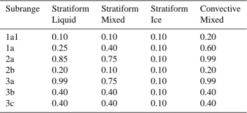
Ri for SALSA are obtained from Stier et al. (2005) and are

shown in Table 4. As the coefficients are essentially the same for SALSA and M7, the variations between two aerosol mod-els in wet removal rates for aerosols depend mainly on the simulated cloud patterns.

(6)

Table 4. Cloud scavenging parameter Ri for the subranges of SALSA. The coefficients remain the same for whole subrange, with an exception for smallest size section 1a1.

Subrange Stratiform Stratiform Stratiform Convective

Liquid Mixed Ice Mixed

1a1 0.10 0.10 0.10 0.20

1a 0.25 0.40 0.10 0.60

2a 0.85 0.75 0.10 0.99

2b 0.20 0.10 0.10 0.20

3a 0.99 0.75 0.10 0.99

3b 0.40 0.40 0.10 0.40

3c 0.40 0.40 0.10 0.40

2.5.2 Dry deposition

Dry deposition velocity is calculated using a serial resis-tance analogy. The resisresis-tance analogy calculates the depo-sition velocity as inverse of the resistance at the surface

vd=r−1, where the resistancer is parameterised from the surface properties according to the scheme of Ganzeveld and Lelieveld (1995) and Ganzeveld et al. (1998). The dry depo-sition flux is calculated using

Fd=Cρairvd, (4)

whereC is the number mixing ratio,ρair is the air density andvdis the dry deposition velocity. The key obstacle in cal-culating the dry deposition flux is calcal-culating the deposition velocity, which ties together all relevant processes involved.

For gas-phase compounds, the total apparent resistance at the surface is divided into three parts: aerodynamicalra, quasi-laminarrband surfacersresistances. The aerodynamic resistancera is calculated in ECHAM5. The quasi-laminar, or boundary layer, resistance is determined from the kine-matic viscosity of the air. The third term, surface resistance, is prescribed for most of the trace gases. Only for SO2, it is calculated using a parameterisation depending on pH, rela-tive humidity, surface temperature and the canopy resistance (Stier et al., 2005). The total resistance is the sum of the three resistances.

In both M7 and SALSA, the calculation of aerosol parti-cle dry deposition uses the big leaf method, withr=ra+

rs. The aerosol deposition is calculated on-line using the aerosol number and mass to calculate the aerosol deposi-tion velocity as a funcdeposi-tion of particle wet radius, density, turbulence and surface cover, as in Stier et al. (2005). A more detailed description of wet deposition can be found in Kerkweg et al. (2006).

2.5.3 Sedimentation

Aerosol particles within the atmosphere are drawn towards the surface by gravitation – this process is known as sedi-mentation. Sedimentation velocity is calculated using Stokes

law (Seinfeld and Pandis, 2006):

F =3π µRpU∞

Cc

, (5)

whereRp is the particle wet radius,µ is air viscosity,U∞ is wind velocity and Cc is the Cunningham slip correction factor. The particle radius is assumed equal to the sectional mean radius after the water uptake.

The calculation of sedimentation relies on the radii of the particles, and therefore the deposition velocities for different internally mixed compounds are the same. As the calculated sedimentation velocity might break the Courant-Friedrich-Lewy stability criterion, the sedimentation velocity is lim-ited tov≤1z

1t, where1tis the timestep length and1zis the

model layer thickness.

2.6 Emissions

The emission module originally made for M7 has been rewritten for SALSA to produce input suitable for a sectional model, while keeping the emission routines otherwise intact. Sea salt, dust and oceanic DMS emissions are calculated on-line. For anthropogenic emissions we have used the Aero-Com year 2000 emission inventory (Dentener et al., 2006) with modifications by Stier et al. (2005), even though the simulation runs were made using meteorology for year 2008. As both M7 and SALSA runs have emissions for the same year, this should not cause significant differences between the experiments. However, when comparing to actual obser-vations for year 2008, the emissions from year 2000 may cause discrepancies.

2.6.1 Carbon emissions

Carbonaceous particulate emissions are emitted into sub-ranges 1a, 2a or 2b, assuming lognormal distributions by Stier et al. (2005) with a median particle radiusr¯=0.075 and standard deviationσ=1.59 (adapted from the AeroCom distributions by Dentener et al. (2006) which haver¯=0.04 andσ=1.8).

There are three different emission sources for black car-bon: biofuel, wildfire, and fossil fuel. Black carbon is as-sumed insoluble, and as such it is emitted to sections within subrange 2b only.

(7)

2.6.2 Sulphur emissions

Sulphur is emitted to the atmosphere mainly as SO2 from natural and anthropogenic sources. Sulphur is naturally emit-ted to the atmosphere mainly by continuous and explosive volcanic activity, and as dimethylsulfide emitted from both oceanic and terrestrial sources. Anthropogenic sources of SO2include wild fires, fossil fuel and biofuel.

Emissions from volcanic sources are based on GEIA in-ventory (http://www.igac.noaa.gov/newsletter/22/sulfur.php; http://www.geiacenter.org/) (Andres and Kasgnoc, 1998). Most of the anthropogenic sulphur – 97.5 % – is emitted as SO2and 2.5 % is emitted as particulate matter SO4(Dentener et al., 2006). In the standard version of SALSA, the primary particles are emitted to subranges 1a, 2a and 3b following the modal structure published by Dentener et al. (2006). How-ever, to facilitate the comparison to M7, the primary emis-sions are in this study described using the M7 modal param-eters (Stier et al., 2005).

Sulphur is emitted to the second lowest model level. Orig-inal 1×1◦ gridded data are remapped to model resolution 1.9×1.9◦using area-weighted averaging.

Emissions of oceanic DMS are calculated on-line by using the Nightingale et al. (2000) parameterisation for air-sea ex-change transfer velocities and simulated 10 m wind speeds. Continental DMS emissions are prescribed as reported by Pham et al. (1995).

2.6.3 Sea salt emissions

The sea salt emission scheme has been modified compared to the M7 and therefore we provide a more detailed description of these emissions.

Sea spray droplets are produced by mechanical tearing of waves or by bursting of bubbles at the sea surface (e.g. de Leeuw et al., 2011). These mechanisms can be expressed with several different sea spray generation functions that can be found in the literature. Usually these formulae provide a parameterisation of the emission flux as a function of 10 m wind speed. Guelle et al. (2001) estimate that the formula-tion of Monahan et al. (1986) is best suited for small parti-cle range (rdrybelow 4 µm). However, Gong (2003) estimate that for particles under 0.2 µm radius, the Monahan et al. (1986) parameterisation overestimates the number flux, and thus they formulated a new parameterisation for these small particles. For particles with dry radius above 4 µm and below 18.75 µm, we have used the Andreas (1998) formulation. We calculate the emission flux into 2nd and 3rd subranges, and hence we use the combination of all three parameterisations mentioned above. In the following formulae,rstands for ra-dius at RH 80 %, and dry particle mass flux is calculated with

rdry=0.5r80. For radii between 50 nm to 400 nm, the mass fluxes are calculated using the Gong (2003) parameterisation

dF

dr =1.373 U

3.41 10 r

−A₍₁₊₀_.₀₅₇_r3.45₎₁₀1.607e−B2

, (6)

when 0.05 µm≤r≤0.4 µm,

where A=4.7(1+2r)−0.017r−1.44 and B=(0.433− log r)/0.433.2 is a fitting parameter that can be used to adjust the emissions below 0.2 µm. U10 is the windspeed at 10 m height. According to Gong (2003), changing the parameter2from 30 to 15 can increase the number concen-trations as much as one order of magnitude and values 30–40 produce similar emissions. Hence, we have used 2=30, which will cause underestimation rather than overestimation. In the 400 nm to 8 µm range, the mass flux is calculated using the Monahan et al. (1986) formulation

dF

dr =1.373U

3.41 10 r

−3₍₁₊₀_.₀₅₇_r1.05₎₁₀1.19e−B2

, (7)

when 0.4 µm≤r≤8 µm,

whereB=(0.380−logr)/0.650.

For the largest particles with radii over 8 µm, we use the Andreas (1998) parameterisation

dF

dr =C U10r

−1_, _when_r_≥_{8 µm}_, ₍₈₎

where the parameterCis calculated from the boundary con-dition that Eq. (7) at its upper limit must equal with Eq. (8) at its lower limit.

Following these parameterisations we calculate the num-ber and mass fluxes using 10 m wind speeds in the range from 0 to 32 m s−1. The fluxes are calculated by integrating over each section separately. The number flux within a section is calculated from the mass flux using the sectional mean diam-eter.

2.6.4 Dust emissions

Mineral dust is found throughout the atmosphere either as fine grained silt or as coarse grained minerals and is lifted to the atmosphere by the surface winds. Higher wind speeds in-crease the amount and also the size of emitted dust particles. Dust emissions are calculated online using the parameter-isation by Tegen et al. (2002). Dust flux is calculated online using 10 m wind speeds, soil clay content and soil moisture from ECHAM5. Both SALSA and M7 use the same parame-terisation. The Tegen et al. (2002) parameterisation gives the flux in sectional space, which is then mapped to M7 modal structure. To produce minimal differences between the mod-els, we use the M7 modal formulation of the flux, which is then mapped to SALSA sections. In SALSA, mineral dust is emitted to subranges 2b and 3c.

2.7 Radiation

(8)

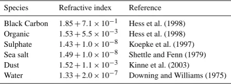
Table 5. Complex refractive indices by compound atλ=550 nm.

Species Refractive index Reference

Black Carbon 1.85+7.1×10−1 Hess et al. (1998)

Organic 1.53+5.5×10−3 Hess et al. (1998)

Sulphate 1.43+1.0×10−8 Koepke et al. (1997)

Sea salt 1.49+1.0×10−8 Shettle and Fenn (1979)

Dust 1.52+1.1×10−3 Kinne et al. (2003)

Water 1.33+2.0×10−7 Downing and Williams (1975)

Instead, the needed aerosol properties have been calculated beforehand for 24 spectral bands, as shown by Toon and Ackerman (1981). These precalculated values are provided for ECHAM5-HAM as lookup tables with three dimensions: Mie parameterα=2π r/λ, and the real and imaginary re-fractive indicesnr andni. For the Mie parameter, r is the

mean radius of a section and λ is the wavelength. The compound specific complex refractive indicesnrandni are

shown in Table 5.

Each model bin can have varying mixing ratios of differ-ent chemical compounds. Therefore, we approximatenrand

ni by volume-weighted average of the refractive indices of

individual compounds including aerosol water. As reported by Lesins et al. (2002), the error in AOD when using this volume-weighted approach can reach up to 15 % in the ex-treme case of black carbon and water.

From the lookup tables the module retrieves the extinction cross section, single scattering albedo and asymmetry factor. Using these values, the aerosol optical depth and ˚Angstr¨om exponent are then calculated for each bin at each grid point.

3 Comparison to previous model studies

3.1 Budgets of aerosol species

Aerosol budgets and lifetimes give us an overview of the cy-cling of different compounds. The compound-specific global aerosol budget varies both spatially and temporally.

We have compared the simulated global budget of aerosols between SALSA and M7. To put the results in a context, we have also provided corresponding values reported by Liu et al. (2005b) and Textor et al. (2006). As Textor et al. (2006) focus on particulate species, we have also included results from the Liu et al. (2005b) for reference for the gaseous species within the sulphur cycle. The overview of aerosol lifecycles is presented in Tables 6 and 7. Table 6 summarises the global sulphur cycle for ECHAM5-HAM with SALSA and M7 and Table 7 summarises the aerosol budget for black carbon, organic carbon, sea salt and dust.

3.1.1 Sulphur

Overall, the burdens of sulphur compounds (Table 6) are very similar to those for SALSA and M7. The simulated

burden of particulate SO4is the same with SALSA and M7 at 0.64 Tg(S). This value is only 0.02 Tg (3.0 %) smaller than the one reported in the AeroCom comparison where the mean for 16 models is 1.99 Tg(SO4), which corresponds to 0.66 Tg(S) (Textor et al., 2006, see Table 10.). SALSA shows four times higher mass of nucleated SO4than M7. This is mostly explained by the model structure. In SALSA the nu-cleated mass of sulphur includes also the sulphur consumed by growth of freshly nucleated particles from approximately 1 nm to 3 nm in diameter.

For the particulate SO4 the difference between the mod-els is caused mainly by aqueous chemistry, a process in which SO2 is oxidised in clouds to produce particulate SO4. Additionally there are small differences in conden-sation, which contributes roughly one quarter of the par-ticulate phase sulphur. The contribution of condensation is only 0.62 Tg yr−1_{(2.7 %) higher with SALSA than with M7.} While the pathways to particulate SO4are clearly different, the global average burdens for SO4 particles are the same with both models. As for the removal processes, dry deposi-tion of SO4with both SALSA and M7 is lower than reported by either Liu et al. (2005b) or AeroCom. On the other hand, wet deposition with SALSA is at the upper bound of and with M7 higher than the model spread reported by Liu et al. (2005b). Despite these mismatches in the removal processes between SALSA and earlier studies, the total burden is al-most the same as in the AeroCom comparison and within the variation of Liu et al. (2005b). The lower sources therefore seem to be compensated with lower sinks.

The overall burden of sulphur associated with gas phase H2SO47×10−4Tg is 22 % smaller than with M7. This dif-ference is caused by difdif-ferences in sources and sinks. While M7 uses all the available H2SO4 for condensation and nu-cleation, in SALSA the amount depends on the equilibrium mass transfer between particles and gas phase H2SO4.

(9)

Table 6. Annual mean global sulphur cycle calculated using SALSA and M7 as well as results found in the literature. Additionally, the

simulated annual mean cover of low (1013–750 hPa), middle (740–460 hPa) and high (440–50 hPa) clouds is included.

SALSA M7 Liu et al. (2005b) AeroCom

(Textor et al., 2006)

SO4particle phase

Burden (Tg S) 0.64 0.64 0.53–1.07 0.66

Sources (Tg S yr−1₎

Total 69.23 79.59 59.67

Emissions 1.77 1.77 0.0–3.5

Condensation 23.40 22.78

Nucleation 0.60 0.16

Aqueous oxidation 43.47 54.88 24.5–57.8 Sinks (Tg S yr−1) 60.92 77.95

Wet Deposition 59.46 75.38 34.7–61.0 53.0

Dry Deposition 1.47 2.42 3.9–18.0 7.23

Sedimentation 0.002 0.15

Lifetime (days) 3.61 2.92 4.12

H2SO4gas phase

Burden (Tg S) 0.0007 0.0009 Sources (Tg S yr−1)

Total 27.88 23.06

SO2+ OH 25.47 20.41

DMS + OH 2.41 2.65

Sinks (Tg S yr−1)

Total 24.07 23.01

Wet Deposition 0.064 0.048 Dry Deposition 0.017 0.024

Condensation 23.40 22.78

Nucleation 0.60 0.16

Lifetime (minutes) 14.11 20.16

SO2

Burden (Tg S) 0.64 0.87 0.20–0.61

Sources (Tg S yr−1)

Total 92.10 94.75

Emissions 71.03 71.03

DMS + NO3 4.86 5.39

DMS + OH 16.21 18.34

Sinks (Tg S yr−1)

Total 89.98 93.22

Wet Deposition 3.66 2.62 0.0–19.9

Dry Deposition 17.38 15.32 16.0–55.0

SO2+ OH 25.47 20.41 6.1–16.8

Aqueous oxidation 43.47 54.88 24.5–57.8

Lifetime (days) 2.55 1.96 0.6–2.6

DMS

Burden (Tg S) 0.08 0.09 0.02–3.0

Sources (Tg S yr−1)

Total 23.46 26.37 10.7–23.7

Sinks (Tg S yr−1)

Total 23.48 26.38

DMS + NO3 4.86 5.39

DMS + OH 18.62 21.00

Lifetime (days) 1.21 1.21 0.5–3.0

Cloud cover

Low clouds 0.17 0.19

Mid clouds 0.17 0.15

(10)

Table 7. Annual mean global black carbon, organic carbon, sea salt and dust budgets calculated using SALSA and M7 together with budgets

found in the literature. For Liu and AeroCom, sedimentation is included in dry deposition.

SALSA M7 Liu et al. (2005b) AeroCom multimodel mean (Textor et al., 2006)

Black carbon

Burden (Tg) 0.07 0.10 0.12–0.29 0.24

Sources (Tg yr−1)

Emissions 7.71 7.71 11.90

Sinks (Tg yr−1) 3.56 7.77 13.14

Wet deposition 3.08 7.14 7.8–13.7 10.51

Dry deposition 0.47 0.61 1.6–4.6 2.63

Lifetime (days) 3.84 4.96 3.3–8.4 7.12

Organic carbon

Burden (Tg) 0.96 0.93 0.95–1.8 1.70

Sources (Tg yr−1)

Emissions 66.13 66.13 96.60

Sinks (Tg yr−1) 54.58 66.32 105.49

Wet 49.88 61.16 86.87

Dry Deposition 4.66 4.97 18.62

Lifetime (days) 5.30 5.14 3.9–8.4 6.54

Sea salt

Burden (Tg) 11.73 12.56 3.41–12.0 7.52

Sources (Tg yr−1)

Emissions 7429.2 6234.8 1010–8076 16 600.00

Sinks (Tg yr−1) 7446.5 6277.3 13915

Wet Deposition 3054.6 3330.8 2168

Dry Deposition 1693.4 1328.0 11 747

Lifetime (days) 0.58 0.74 0.19–0.99 0.48

Dust

Burden (Tg) 13.11 19.3 4.3–35.9 19.20

Sources (Tg yr−1)

Emissions 720.4 1603.4 820–5102 1840.0

Sinks (Tg yr−1) 937.7 1649.3 2172.48

Wet Deposition 439.9 961.8 486–4080 560.64

Dry Deposition 106.4 116.3 183–1027 1611.84

Lifetime (days) 6.64 4.39 1.9–7.1 4.14

Water soluble fraction in 3c

Burden (Tg) 0.0087 N/A

Sources (Tg yr−1)

Emissions N/A

Sinks (Tg yr−1) 0.32

Wet Deposition 0.26

Dry Deposition 0.016

Sedimentation 0.046

(11)

Despite the nudging method, the global annual mean 10 m wind speeds are 4 % lower with SALSA than with M7, which causes 11 % lower emissions of DMS with SALSA. As DMS is globally a large source of sulphur, lower DMS leads to slightly lower mass of SO2and SO4. However, the emissions with SALSA are at the upper bound of the variation in the emission of DMS as reported by Liu et al. (2005b).

3.1.2 Organic carbon

As the prescribed emissions of organic carbon are the same for SALSA and M7, there is no difference between the mod-els in this respect. The atmospheric burden of organic carbon (OC) at 0.96 Tg differs by only 0.03 Tg (3 %) from the bur-den simulated with M7 (0.93 Tg). As the organic carbon mass in SALSA is associated only with subranges 1 and 2, the close agreeement between the models suggests that most of the OC is in particles below 700 µm in diameter also in M7. In the AeroCom comparison the mean of particulate organic matter is found to be 1.7 Tg, which corresponds to 1.21 Tg (OC) being 21 % higher than with SALSA. While the bur-den is practically the same for M7 and SALSA, the 20 % (11.55 Tg) lower removal of organic carbon in SALSA indi-cates that part of the mass is transferred to subrange 3 where it is not explicitly tracked and thus implies that the burden should be even little higher with SALSA. This is also seen in SALSA as lower sedimentation of organic carbon particles, which mainly affects very large aerosols. The loss by sedi-mentation is 2.5 times smaller because only sedisedi-mentation of OC is tracked only for particles under 700 nm. In compari-son to observations, organic carbon mass is underestimated in most global aerosol-climate models (Jathar et al., 2011) and we would expect to the same for SALSA.

3.1.3 Black carbon

Similarly to organic carbon the emissions of black carbon are the same with both models. The burden of black car-bon in SALSA is 0.07 Tg which is 0.03 Tg lower than that of M7. Both models simulate a lower burden than any of the studies mentioned by Liu et al. (2005b) and clearly lower than the mean of the models participating in the AeroCom intercomparison. However, even in the AeroCom compari-son ECHAM5-HAM had the lowest BC burden of all models which is probably due to lower emissions of carbonaceous material than in the other models. Similarly to organic car-bon the removal of black carcar-bon is lower in SALSA than in M7 being less than half of the emitted mass. Removal being clearly lower than emissions implies that a relatively large portion of particles containing BC are grown to subrange 3 and the actual burden might be within the variation reported by Liu et al. (2005b). The growth of black carbon to 3rd sub-range is partly caused by a low removal of insoluble particles by wet deposition thereby increasing the time for growth of particles.

3.1.4 Sea salt and mineral dust

A large portion of the mass of sea salt and mineral dust is in particles larger than 700 nm in diameter. The mass of parti-cles in this size range is estimated using the mean diameter of particles and their densities.

Sources for sea salt are significantly higher with SALSA than with M7 which is caused by the new formulation of sea salt emissions while differences in wind patterns may also play a role. The latter cause is evident especially in the South-ern Ocean. Despite the 1200 Tg difference for the emission of sea salt particles, the burden is only 0.83 Tg (6.6 %) smaller with SALSA. However, the sedimentation is 66 % higher with SALSA. Contributions of dry and wet depositions are of similar magnitude (within 9 % and 22 % respectively) in both models. It seems that the large difference in emissions is compensated by larger sedimentation with SALSA.

For dust, however, emission and burden are clearly lower with SALSA than with M7. The emissions with SALSA are less than half (44 %) of the emissions with M7. SALSA emissions are similarly less than half of the amount reported in the AeroCom emission inventory (Dentener et al., 2006). The difference is caused by 7 % lower surface wind speeds over land with SALSA and the calculation of emissions us-ing modal parameters for SALSA sectional structure. Dry removal processes are still quite comparable (9 % lower in SALSA), and the main difference in the total removal rate is due to wet deposition. In SALSA mineral dust is mainly emitted to insoluble sections and therefore has a weaker wet deposition flux. Also the removal by dry deposition and sed-imentation is low especially when comparing with Aero-Com comparison. This might be influenced by fixed sectional diameters in the sub region 3 as sedimentation velocity is strongly dependent on the particle diameter.

The water soluble fraction in the subrange 3c constitutes a very small part of total aerosol loading. Global burden is only 0.0087 Tg which is in the same range as for gas phase H2SO4.

3.2 Lifetimes

We calculated the lifetime of particles by using a relation between source and burden rather than sink and burden. We chose this way because part of the aerosol mass is transferred to subrange 3 which does not include mass tracers. However, there will be some error because the burden does not include particles larger than 700 nm in diameter for OC, BC and SO4. The lifetimes of black carbon and sea salt are shorter with SALSA than with M7, but otherwise M7 predicts shorter life-times. For black carbon and dust the difference in lifetimes between models exceeds one day.

(12)

When comparing to the AeroCom multimodel mean, the largest difference is found for black carbon, which is mostly caused by the coagulation or growth losses to particles larger than 700 nm in diameter in SALSA. Lower burden and re-moval by dry and wet deposition and sedimentation than in the other models could indicate that a large fraction of the material is removed by the processes affecting particles grown over the 700 nm boundary in the aerosol model.

Even though the sea salt emissions are higher, the lifetime of particles is shorter with SALSA than with M7 because the removal rate of sea salt is increased. This increase in removal is mainly due to higher sedimentation in SALSA than in M7, thereby resulting in 21.6 % smaller lifetime than with M7.

For dust, the lifetime with SALSA is 2.45 days lower than with M7 but the proportional significance of different removal processes are rather consistent with M7, while the emissions are less than half of those simulated with M7 and little less than in other studies previously reported (Liu et al., 2005b; Textor et al., 2006).

3.3 Spatial distribution of aerosol mass

Figure 2 shows the annual mean of vertically integrated col-umn mass of the compounds in particulate phase. Aerosol mass distribution of different compounds varies depending on the properties of the compound, as can be seen in Fig. 2. Removal and transport depends largely on the composition of particles, and particles consisting of mainly water soluble material are more prone to be removed by wet deposition, while fine insoluble particles will more probably be trans-ported further from the source.

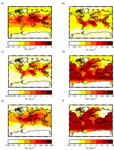
Sulphate is seen in large areas over both land and ocean. The wide dispersal of SO4 results from SO2 dispersion throughout the atmosphere and its oxidation to H2SO4 and consequent nucleation and condensation. Regions with high-est burdens for organic carbon coincide with strong emission areas, as most of the global organic carbon is found in the South America and Central Africa. The column burden of sea salt is naturally high over the oceans. However, there are also relatively high burdens in some parts of, e.g. Australia, South-America and East-Coast of Africa, indicating trans-ports inland. Sea salt burden is the highest in the Southern Ocean, which has reportedly very high windspeeds (Yuan, 2004) producing large amounts of sea salt. By comparing sea salt and aerosol water burdens in Fig. 2d and f, we can see that a large part of aerosol water is associated with sea salt aerosols.

Dust burden is highest near large deserts. Most promi-nently the dust emissions from deserts are seen over Sahara, while also Asian and Australian deserts show large dust bur-den. The transport of Saharan dust all the way to Amazonia can be seen in the model, a phenomenon that has also been observed by Gilardoni et al. (2011).

Fig. 2. Annual mean of vertically integrated column mass for year

2008 for (a) sulphate (SO4), (b) organic carbon (OC), (c) black car-bon (BC), (d) particulate water (WAT), (e) dust (DU) and (f) sea salt (SS) simulated with SALSA. All units are mg m−2.

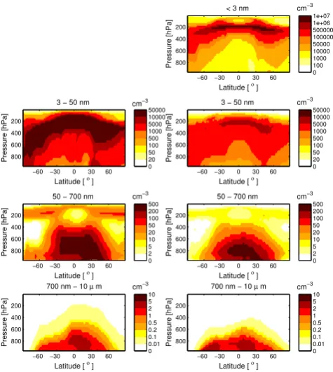
3.4 Vertical distribution

In Fig. 3 we show the annual mean of the zonally averaged number concentrations for SALSA (left hand panels) and M7 (right hand panels). The M7 number concentrations are cal-culated for SALSA subrange diameter ranges to facilitate comparison. Additionally, we have plotted the M7 number concentrations of particles below the lower limit of SALSA in the topmost panel on the right hand side.

In Fig. 3a we can see that especially in the upper tro-posphere, the binary nucleation creates an extremely high amount of particles in M7 that do not show up in SALSA due to their inability to grow over 3 nm in diameter, which is the low cut-off diameter of SALSA’s size distribution.

(13)

Pressure [hPa]

Latitude [ ο ] < 3 nm

−60 −30 0 30 60 200 400 600 800 cm−3 0 100 1000 10000 50000 100000 500000 1e+06 1e+07 Pressure [hPa]

Latitude [ ο ] 3 − 50 nm

−60 −30 0 30 60 200 400 600 800 cm−3 0 20 50 100 500 1000 5000 10000 50000 Pressure [hPa]

−60 −30 0 30 60 200 400 600 800 cm−3 0 2 5 10 20 50 100 200 500 Pressure [hPa]

Latitude [ ο_]

700 nm − 10 µ m

−60 −30 0 30 60 200 400 600 800 cm−3 0 0.01 0.1 0.2 0.5 1 2 5 10 Pressure [hPa]

Latitude [ ο_]

700 nm − 10 µ m

−60 −30 0 30 60 200 400 600 800 cm−3 0 0.01 0.1 0.2 0.5 1 2 5 10

Fig. 3.Annual means of zonally averaged global vertical concentration distribution of particles. Left hand

panels show concentrations with SALSA and right hand panels show the M7 concentrations mapped to SALSA subrange structure. Each panel corresponds to one subrange of SALSA: from the top 1,2,3. For M7 the top most panel shows particle concentrations below the 3 nm lower limit of SALSA.

49

Fig. 3. Annual means of zonally averaged global vertical

concentra-tion distribuconcentra-tion of particles. Left hand panels show concentraconcentra-tions with SALSA and right hand panels show the M7 concentrations mapped to SALSA subrange structure. Each panel corresponds to one subrange of SALSA: from the top 1, 2, 3. For M7 the topmost panel shows particle concentrations below the 3 nm lower limit of SALSA.

the particles do not grow enough to show up in the 3–50 nm range.

In the 200 hPa region of subrange 2, SALSA has concen-trations of 20–100 cm−3while M7 has concentrations below 10 cm−3. This difference is probably a result from having four size classes in SALSA and one or two modes with M7, thereby producing more accurate description for removal processes in SALSA than in M7. In addition, with SALSA the particle concentrations in the boundary layer are higher at high latitudes, with concentrations of 20 to 50 cm−3 as compared to 0 to 10 cm−3 with M7. Near the equator the concentration maximums are closer but SALSA still shows more particles than M7.

In the 3rd subrange the concentrations are relatively sim-ilar with both models. However, with SALSA the particles are transported higher and M7 shows slightly higher concen-trations in the 200–600 hPa region. In the Southern Hemi-sphere (60◦S to 30◦S) the surface concentrations with M7 are higher in this size range. In this region SALSA shows only 2–5 cm−3 while M7 has values 2–10 cm−3. In this re-gion, most of the particles are sea salt and it seems that in SALSA the sea-salt particles are larger and fewer, which may be caused by the fixed diameters used in the 3rd diameter range.

10−2 10−1 100 101 10−2

10−1 100 101

Observed OC [µ g m−3_]

Modeled OC [

µ g m −3] a) IMPROVE EMEP IMPROVE mean EMEP mean

10−2 10−1 100 101 10−2

10−1 100 101

Observed BC [µ g m−3_]

Modeled BC [

µ g m −3] b) IMPROVE EMEP IMPROVE mean EMEP mean 10−2 10−1 100 101 10−2 10−1 100 101

Observed SO4[µ g m −3 ] Modeled SO 4 [ µ g m −3] c) IMPROVE IMPROVE mean 10−3 10−2 10−1 100 101 10−3 10−2 10−1 100 101

Observed SS [µ g m−3

]

Modeled SS [

µ g m −3] d) IMPROVE IMPROVE mean

Fig. 4. Scatterplot of simulated and observed annual mean surface concentrations of organic carbon, black

carbon, sulphate and sea salt. Red circles indicate comparison with IMPROVE network and blue squares

represent EMEP network. Black symbols represent mean values of respective symbols. Solid line indicates 1:1

ratio between observations and simulated values. Similarly dot-dashed line indicates 1:2 and 2:1 ratios, and

dotted lines indicate 1:10 and 10:1 ratios.

50

Fig. 4. Scatterplot of simulated and observed annual mean surface

concentrations of organic carbon, black carbon, sulphate and sea salt. Red circles indicate comparison with IMPROVE network and blue squares represent EMEP network. Black symbols represent mean values of respective symbols. Solid line indicates 1:1 ratio between observations and simulated values. Similarly dot-dashed line indicates 1:2 and 2:1 ratios, and dotted lines indicate 1:10 and 10:1 ratios.

4 Comparison to surface measurements

4.1 Surface concentrations of particulate mass

(14)

lower than 2.5 µm. The modelled mass concentration of sul-phate, organic and black carbon is accounted for particles under 700 nm in diameter while the modeled mass concen-trations of sea salt includes all smaller than 1.7 µm in diam-eter (bins 2a1–3a1). The sea salt size range is chosen to cor-respond to the PM2.5 data available from the stations. The mean fractional bias (MFB) showing the overall deviation of the modelled concentrations from the observations of the IMPROVE network are shown in Table 8. MFB indicates that performance with SALSA is lower than M7 for organic car-bon, while for other species performance is slightly better.

For the organic carbon mass concentrations (Fig. 4a), we can see that SALSA underestimates the surface concentra-tions. Out of the 117 comparison pairs, 45 (36.5 %) are within a factor of two of the IMPROVE network data. On the other hand, in only 12 (10.3 %) cases the discrepancy is over one order of magnitude. For EMEP data, the simu-lated concentrations fall within one order of magnitude at all of the seven sites. For IMPROVE, the mean simulated mass concentrations (0.80 µg m−3) is within a factor of two of the observed mean (1.05 µg m−3), and for EMEP with a factor of three (simulated 1.02 µg m−3, observed 2.79 µg m−3) M7 shows slightly lower mean concentrations (0.73 µg m−3 for IMPROVE and 0.93 µg m−3for EMEP) than SALSA.

The simulated black carbon mass concentration mean (Fig. 4b) for gridpoints corresponding to the IMPROVE sites is 0.15 µg m−3(0.16 µg m−3with M7) which is 23 % lower than the observed mean of 0.20 µg m−3. In 43 of the 117 cases (36.7 %), the simulated concentration is within a fac-tor of two of the observed concentration. There are 17 grid-points where the concentration differs by more than by a factor of 10 from the observation. Thus, between the IM-PROVE sites there is large variation in model performance, while on average the model captures concentrations quite well. The simulated mean of black carbon mass for EMEP sites is 0.39 µg m−3(0.38 µg m−3 for M7) underestimating the observed mean of 0.85 µg m−3 by 54 %. The black car-bon budget suggests that the underestimation is partly due to the mass associated with particles with diameter over 700 nm (Table 7).

In Fig. 4c, the scatterplot for SO4is shown. In 58 (49.6 %) cases the simulated concentration is within a factor of two of the IMPROVE observations. The mean simulated concen-tration of SO4is 0.75 µg m−3(0.66 µg m−3with M7). It is within a factor of two of the mean of observed concentra-tions (1.27 µg m−3_{). The concentrations exceeding 1 µg m}−3 are underestimated using SALSA by over one order of mag-nitude at three gridpoints. However, the modelled sulphate mass is only tracked only up to the diameter of 700 nm while the observations include particles up to 2.5 µm which partly explains the low concentrations.

Both observed and simulated sea-salt mass concentrations (Fig. 4d) exhibit high variation. The simulated concentrations have a mean of 0.045 µg m−3(0.16 µg m−3with M7) under-estimating the observed mean of 0.13 µg m−3 by 65 % for

1 10 100 1000

101 102 103 104

dp[nm]

dN/dlog d

p

[cm

ï

3 ]

a) Pallas

1 10 100 1000

101 102 103

104 b) Jungfraujoch

dp[nm]

dN/dlog d

p

[cm

ï

3 ]

1 10 100 1000

101 102 103 104

dp[nm]

dN/dlog d

p

[cm

ï

3 ]

c) Aspvreten

1 10 100 1000

101 102 103 104

dp[nm]

dN/dlog d

p

[cm

ï

3 ]

d) Melpitz

1 10 100 1000

101 102 103 104

dp[nm]

dN/dlog d

p

[cm

ï

3 ]

e) Mace Head

1 10 100 1000

101 102 103 104

dp[nm]

dN/dlog d

p

[cm

ï

3 ]

f) Hyytiala

Obs median Obs 95% Obs 5% M7 binary SALSA binary SALSA activation

Fig. 5. Observed and simulated annual median size distributions for six measurement stations(a)Pallas,

(b)Jungfraujoch,(c)Aspvreten,(d)Melpitz,(e)Mace Head and(f)Hyyti¨al¨a. Simulated size distribution for M7 is plotted in blue solid line. Simulated size distributions for SALSA are plotted with red solid line indicating activation type nucleation and with red dashed line for binary nucleation. Observed annual median size distributions are plotted in black, with dashed black lines showing the 95th and 5th percentiles of observed concentrations (Asmi et al., 2011).

51

Fig. 5. Observed and simulated annual median size distributions

for six measurement stations (a) Pallas, (b) Jungfraujoch, (c) As-pvreten, (d) Melpitz, (e) Mace Head and (f) Hyyti¨al¨a. Simulated size distribution for M7 is plotted in blue solid line. Simulated size distributions for SALSA are plotted with red solid line indicating activation type nucleation and with red dashed line for binary nu-cleation. Observed annual median size distributions are plotted in black, with dashed black lines showing the 95th and 5th percentiles of observed concentrations (Asmi et al., 2011).

Table 8. Simulated mean fractional bias between observations at

IMPROVE stations and modelled values with SALSA and M7 for organic carbon, black carbon sulphate and sea salt.

SALSA M7

OC −0.254 −0.162 BC −0.242 −0.248 SO4 −0.192 −0.261

SS −0.102 0.418

the IMPROVE sites. Out of the 117 cases, only 36 (30.8 %) are within a factor of two of the observed concentrations. The discrepancy between the observed and simulated con-centrations can be as much as two orders of magnitude. The underestimation in larger particles may be partly due to the coarse sectional structure and partly due to the inadequately described transport to continental sites in the module.

4.2 Particle size distributions and number concentrations over Europe

(15)

a subset of these measurements to the size distributions simulated with SALSA and M7. Figure 5 shows the mod-elled and observed annual median aerosol size distributions at six EUCAARI sites: Jungfraujoch (Jurnyi et al., 2011), Hyytiälä (Hari and Kulmala, 2005), Mace Head (Jennings et al., 1991), Aspvreten (Tunved et al., 2004), Melpitz (En-gler et al., 2007) and Pallas (Lihavainen et al., 2008). These sites include coastal (Mace Head), mountain (Jungfraujoch), arctic (Pallas), boreal coniferous (Hyytiälä), urban polluted (Melpitz) and mixed boreal coniferous and deciduous (As-pvreten) locations. For SALSA we have plotted the size dis-tributions from simulations using either binary or activation nucleation mechanisms, while for M7 only binary nucleation mechanism is available.

When the activation-type boundary layer nucleation is used, the concentration of small particles increases. This leads to a better agreement with observations of particles smaller than 50 nm in diameter than using only binary nu-cleation, which is in line with earlier studies with activation-type nucleation (e.g. Spracklen et al., 2010; Kazil et al., 2010). The concentrations produced using binary nucleation only in either of the models are significantly lower than ob-served. At the selected sites, there is little or no difference in the concentrations of particles larger than 80 nm in diameter between the binary or activation-type nucleation simulations with SALSA. This indicates that the concentrations of parti-cles in this size range depends heavily on the primary emis-sions and the higher concentrations of small particles with activation-type nucleation do not grow this large. Note that the modelled growth of nucleation mode particles could be increased with the inclusion of organic vapors.

Both SALSA and M7 show similar concentrations when using binary nucleation at four of the six sites. At Jungrau-joch and Mace Head the Aitken mode particles have very low concentrations with SALSA, but the concentration is in-creased when using activation-type nucleation. However, the increased concentrations of these particles have very limited effect on the concentration of particles 50 nm–100 nm in di-ameter.

In Fig. 5c, d and e we see that the concentrations of par-ticles 100 nm to 300 nm in diameter are clearly higher with SALSA than with M7. For this size range, SALSA is closer to the observed concentrations, while it has trouble predict-ing the concentrations of particles 50 nm–100 nm in diame-ter, as seen in observations and simulation with M7. This is possibly caused by scavenging of small particles by coagula-tion and too low condensacoagula-tional growth of smaller particles.

The particles 100 nm–500 nm in diameter contribute most of the cloud condensation nuclei concentration, and there-fore this size range is important for cloud activation studies. The cloud activation occurs mainly in diameter range 50 nm– 200 nm; and compared to M7, SALSA shows better agree-ment to observations for these particles in polluted regions and worse agreement in regions with clean air. However, the simulated concentrations remain lower than the observed,

101 102 103 104 0 0.01 0.02 0.03 0.04 0.05

0.06 f) Hyytiala

N100 concentrations [cm −3 ] Frequency 100 101 102 103 104 0 0.01 0.02 0.03 0.04 0.05 0.06 a) Pallas

N100 concentrations [cm −3 ] Frequency 101 102 103 104 0 0.02 0.04 0.06 0.08 d) Melpitz

N100 concentrations [cm −3 ] Frequency 101 102 103 104 0 0.01 0.02 0.03 0.04 0.05 0.06 c) Aspvreten

N100 concentrations [cm −3 ] Frequency 101 102 103 104 0 0.05 0.1 0.15 0.2 b) Jungfraujoch

N100 concentrations [cm −3 ] Frequency 101 102 103 104 0 0.02 0.04 0.06 0.08

0.1 e) Mace Head

N100 concentrations [cm −3

]

Frequency

M7 obs SALSA binary SALSA activation

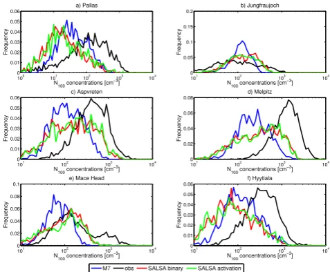
Fig. 6.Histograms ofN100concentrations at six EUCAARI stations. The concentration bins are evenly

dis-tributed in the logarithmic concentration axes. Y-axis shows the relative fraction of each bin compared to total

number of valid measurements.

52

Fig. 6. Histograms ofN100 concentrations at six EUCAARI

sta-tions. The concentration bins are evenly distributed in the logarith-mic concentration axes. Y-axis shows the relative fraction of each bin compared to total number of valid measurements.

which is probably mainly caused by the missing condensa-tion of organic vapors which has been shown to have a large impact on the growth of particles in this size range (Riipinen et al., 2011).

Figure 6 shows the histograms of total number concentra-tions of 100–500 nm particles (N100) at six EUCAARI sta-tions. The particle diameter of 100 nm corresponds roughly to activation at critical supersaturation of 0.3 % for Finnish background aerosol (Sihto et al., 2010). In four cases SALSA shows wider frequency of concentrations, with higher fre-quencies at the larger concentrations than M7. In Mace Head the high observed concentrations associated with polluted air are not reproduced with either model, while the low concen-trations associated with marine air are well reproduced with SALSA (A. Asmi, personal communication, 2011). This sup-ports the good agreement between SALSA and observa-tions for the marine size distribuobserva-tions (Fig. 8). In Pallas and Hyytiälä, M7 shows histograms slightly closer to observed than SALSA, although the histograms with both models are fairly similar. Overall, SALSA seems to reproduce the ob-served histograms of particles at size range relevant to cloud activation better than M7, indicating its better applicability to cloud activation studies. However, at sites with cleaner air (Pallas and Hyytiälä), M7 performs better. This further indi-cates that with too low simulated growth of particles below 50 nm in diameter,N100depends largely on emissions.

(16)

−90−75−60−45−30−15 0 15 30 45 60 75 900 200

400 600 800 1000 1200 1400 1600

Latitude

Concentration [cm

−3 ]

SALSA (D_p > 20 nm) M7 (D_p > 20 nm) Heintzenberg et al.

Fig. 7.Total annual mean sea surface concentration of particles in 10 latitude bands. Observed size distributions are marked with black, SALSA with red diamonds and M7 in blue squares. The observed mean values for the latitude bands are shown in black circles. As the observations have a lower cutoff diameter of 20nmthe modeled concentrations are shown only for particles larger than 20nmin diameter.

53

Fig. 7. Total annual mean sea surface concentration of particles

in 10 latitude bands. Observed size distributions are marked with black, SALSA with red diamonds and M7 in blue squares. The ob-served mean values for the latitude bands are shown in black circles. As the observations have a lower cutoff diameter of 20 nm the mod-elled concentrations are shown only for particles larger than 20 nm in diameter.

slightly better than M7 and vice versa. Nevertheless, the ef-fect of organic vapors should be studied before the imple-mentation of cloud activation of particles.

4.3 Marine particle number size distributions

Heintzenberg et al. (2000) compiled a data set of marine boundary layer (MBL) aerosol size distributions from three decades of cruise and flight measurements. In their work the size distribution data was presented as log-normal bimodal distribution with a geometric mean diameter, standard devi-ation and number concentrdevi-ation given on both modes. The distributions have been reported for 10 latitude bands. We have plotted the observed data together with simulated con-centrations for SALSA and M7 (Figs. 7 and 8).

Figure 7 shows the average surface concentrations of par-ticles larger than 20 nm in diameter for 10 different latitude bands. SALSA and M7 concentrations are averaged from the same regions as the observations (Fig. 1 in Heintzen-berg et al., 2000). The observed mean values are in the range 370–500 cm−3 while, the simulated values can reach over 1500 cm−3in the Southern Ocean. In this region we can see the largest discrepancy between the module and the observa-tions as the simulated particle concentraobserva-tions for SALSA are 4-fold over the observed values.

In the tropics, SALSA and M7 show similar concentra-tions of particles. In other latitude bands, the concentration with SALSA are higher than those with M7. The largest dif-ference between the models is again seen in the Southern Ocean, where SALSA produces five times higher concen-trations of particles larger than 20 nm in diameter than M7. This difference is seen because the measurement locations

between Antarctica and South America used in the com-parison coincide with a regions with high concentrations of sulphuric acid. The high amount of sulphuric acid causes stronger growth of freshly formed particles by condensation with SALSA than with M7, resulting in high concentrations of particles 20 nm–50 nm in diameter. While M7 predicts a mean marine concentration of 320 cm−3 and thus underes-timates the observed mean concentration of 450 cm−3, the new sea salt formulation of SALSA causes it to overesti-mate the number concentrations with mean of 670 cm−3. De-spite overpredicting the mean concentration, SALSA mostly shows better agreement with the observations than M7. Fur-thermore, SALSA captures the concentrations at the roaring fourties (40◦–49◦S) much better than M7.

The M7 has lower root mean square error of average num-ber concentrations of 184.0 while SALSA has 225.1. With similar and quite large errors, both M7 and SALSA perform equally well.

Simulated and observed particle size distributions in Fig. 8 are shown for annual mean surface concentrations in 12 latitude bands. For the modelled values we use gridpoints corresponding to the 15◦×15◦ gridboxes, as explained by Heintzenberg et al. (2000). Especially for particles 0.01– 0.1µm in diameter, SALSA shows worse agreement with ob-servations than M7; for the particles with diameters ranging 0.1–1µm, SALSA shows better agreement with the observa-tions than M7.

5 Comparison to remote sensing observations

5.1 Aerosol optical depth

The simulated aerosol optical depth (AOD) is compared with satellite and ground-based measurements. The satellite re-trievals include both the Moderate Resolution Imaging Spec-trometer (MODIS) (Remer et al., 2005) and Multi-angle Imaging SpectroRadiometer (MISR) (Martonchik et al., 1998; Kahn et al., 2005) instruments. Because the MODIS AOD over land areas has high uncertainties (Levy et al., 2010; Pinty et al., 2010), we use a composite of the MODIS and the MISR instruments. The MODIS is used for ocean and MISR for land gridpoints. Ground-based measurements are gathered from the AERONET robotic network of sunpho-tometers (Holben et al., 1998).

MODIS and MISR level 3 data, which have a spatial reso-lution of 1×1 degree, were downloaded from NASA’s Gio-vanni (Acker and Leptoukh, 2007) web portal (http://daac. gsfc.nasa.gov/giovanni/). The composite MODIS-MISR an-nual mean is calculated from monthly mean values.