G × E interaction and Stability Analysis of Maize Hybrids Using Eberhart and Russell Model

DOI: 10.30954/0974-1712.03.2019.1

©2019New Delhi Publishers. All rights reserved

GENETICS AND PLANT BREEDING

G × E interaction and Stability Analysis of Maize Hybrids Using

Eberhart and Russell Model

R Nirmal Raj*, C.P. Renuka Devi and J. Gokulakrishnan

Department of Genetics and Plant Breeding, Faculty of Agriculture, Annamalai University, Chidambaram, Tamil Nadu, India

*Corresponding author: [email protected] (ORCID ID: 0000-0002-6444-7106)

Paper No. 757 Received: 15-10-2018 Accepted: 22-01-2019

ABSTRACT

The present study was carried out to identify stable Maize hybrids across various environments as the performance of each hybrid tends to vary when grown in different seasons or locations. Twenty one Maize hybrids and two commercial checks were tested over three locations in India viz., Viluppuram, Trivandrum and Nagercoil. Eberhart and Russell model of stability analysis was carried out which revealed a significant effect of each environment on the hybrids taken, for all the ten morphological traits except the number of leaves. The hybrid AU-101 was identified as a stable hybrid with high mean under less favourable conditions and the hybrid AU-114 was recognized as a stable hybrid under favourable conditions. None of the check hybrids viz., CP-818 and Bioseed-TX369 showed stability in any of the environment. Thus, it emphasized the need for the development of location specific hybrids or a hybrid that is, stable across environments.

Highlights

mEberhart and Russell model of stability analysis is used in this research and assessed the performance of hybrids across the environments.

Keywords: Stability, maize hybrids, environments

In India, Maize is the third most important cereal

crop after Rice and Wheat. It contributes a lion

share to the total food production globally. The

Maize production is estimated at 26.2 million tonnes

(FAOSTAT, 2017) in India and the projected demand

for Maize is expected to be 42 million tonnes by

the year 2025 (Sain Dass

et al.

2009). Corn which

literarily means “that which sustains life” (Akinyele

and Adigun, 2006) has been cultivated throughout

India. The significance of the crop has grown due to

its multipurpose nature and the high yielding maize

hybrids met the quest for higher yield by farmers.

Even with these highly productive hybrids, farmers

experience the distress of inconsistent yield across

different environments.

There is a growing need to identify maize hybrids

that perform uniformly and consistently for yield

regardless of environments. Eberhart and Russell

(1966) stated that a desirable cultivar should have

an average yield performance that is higher under

favourable conditions and less fluctuating under

unfavourable conditions than that of the group of

cultivars when tested in many environments. There

is an ever growing demand for environment specific

hybrids, hence the present study was carried out to

identify stable and environment specific hybrids

and to test the hybrid performance in environment

other than conventional maize growing areas.

MATERIALS AND METHODS

The materials for stability analysis consisted of

twenty one maize hybrids of single cross origin were

received from Department of Genetics and Plant

environments during June, 2017 in a one row trial.

The particulars of three environments are given in

Table 1. Experiments were laid out in randomized

block design with three replications. Fifteen plants

per replication were maintained for each hybrid.

Ten morphological traits

viz.,

days to 50% tasseling,

number of leaves, days to maturity, plant height

(cm), cob placement height (cm), ear length (cm),

number of kernels per row, number of kernels per

ear, hundred seed weight (g) and yield per plant (g)

were recorded from five randomly selected plants

for each hybrid per replication. Linear regression

model of stability suggested by Eberhart and Russell

(1966) was employed and the data was analyzed

using TNAUSTAT software.

RESULTS AND DISCUSSION

The combined analysis of variance revealed

significant differences among the hybrids for all

the traits thus indicated the existence of inherent

genetic variability and suggest the possibility

of selecting a stable hybrid from the lot. Similar

results were reported by Usharani (2012) and

Lata

et al.

(2010). Highly significant genotype х

environment interaction was observed for almost all

the characters except number of leaves indicating

that all the hybrids interacted considerably well

with the environmental conditions (Table 2). Similar

interaction for various traits was also reported by

Admassu

et al.

(2008).

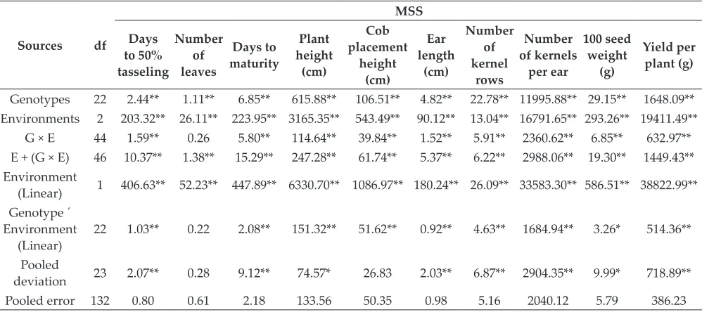
Analysis of variance for Eberhart and Russell

model revealed highly significant E+ (G×E) for all

the characters against pooled error and indicated

distinct nature of seasons and GхE interactions

in the phenotypic expression. Highly significant

values for environment (linear) variance indicated

considerable additive environmental variance for

all the traits. Pooled deviations were also highly

significant for most of the characters except for

number of leaves (Bharathiveeramani

et al.

2016)

and cob placement height which indicated that

unpredictable portion formed the major part of

the GхE interactions. The contribution of linear

portion to GхE interactions was revealed by highly

significant GхE (Linear) variance for nine traits

except number of leaves (Table 3). Similar works

were done by Gami

et al.

(2017) and Matin

et al.

(2017).

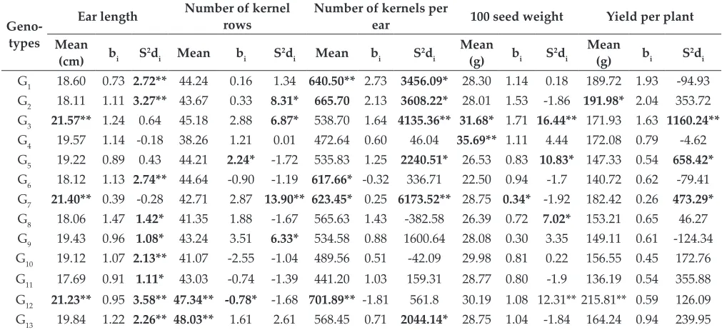
The mean performance, regression (b

) and squared

deviation (s

d

i

) for ten morphological traits are

presented in Table 4a and 4b. It is interesting to

note that no one hybrid was stable for all the

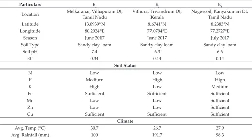
Table 1:

Particulars of three environments

Particulars E1 E2 E3

Location Melkaranai, Villupuram Dt, _{Tamil Nadu} Vithura, Trivandrum Dt, _Kerala Nagercoil, Kanyakumari Dt, _{Tamil Nadu}

Latitude 13.0939°N 8.6741°N 8.2383°N

Longitude 80.2924°E 77.0794°E 77.2727°E

Season June 2017 June 2017 July 2017

Soil Type Sandy clay loam Sandy clay loam Sandy clay loam

Soil pH 7.4 6.3 6.6

EC 0.34 0.14 0.14

Soil Status

N Low Low Low

P Medium High High

K High Low Medium

Fe Sufficient Sufficient Sufficient

Mn Low Low Sufficient

Zn Low Low Sufficient

Cu Sufficient Sufficient Sufficient

Climate

Avg. Temp (°C) 30.7 26.7 27.9

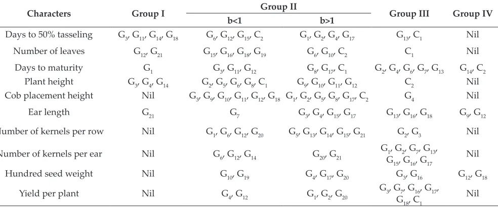
characters. Twenty one hybrids and two checks with

higher/lower mean values than grand mean were

grouped into four based on stability parameters

viz.,

regression coefficient and squared deviation,

according to the methodology followed by Mehra

and Ramanujam (1979) and Singh and Singh (1980)

(Table 5). The hybrids falling in group I have

desirable mean, regression coefficient value around

one with non significant squared deviation. Under

group II, hybrids with less than unity regression

value and non significant squared deviation are

taken, indicating suitability towards unfavourable

environments. Again, the hybrids with more than

unity regression is also classified under group II

indicating the hybrid’s suitability towards favourable

environments. Behaviour of hybrids falling in group

III and group IV cannot be predicted as they exhibit

significant squared deviation, irrespective of the

regression coefficient values.

According to the grouping, the hybrid G14 is stable

for two traits

viz.,

days to 50% tasseling and plant

height, as it was placed under group I. Under

group II (b<1), the hybrid G12 is stable for six

traits

viz.,

days to 50% tasseling, days to maturity,

cob placement height, number of kernels per row,

number of kernels per ear and yield per plant in

unfavourable conditions. The hybrid G20 is placed

under group II (b>1) and is stable in favourable

conditions for three traits

viz.,

number of kernels

per ear, hundred seed weight and yield per plant.

These results are in line with the reports of Kaundal

Table 2:

Combined analysis of variance for ten morphological characters

Sources df MSS Days to 50% tasseling Number of leaves Days to maturity Plant height (cm) Cob placement height (cm) Ear length (cm) Number of kernel rows Number of kernels per ear 100 seed weight (g) Yield per plant

Replication 2 1.30 2.81 2.03 334.25 37.25 1.94 5.58 3040.91 13.49 968.42 Genotype 22 2.44** 1.11** 6.93** 615.78** 106.51** 4.81** 22.77** 11995.67** 29.13** 1648.08** Environment 2 203.32** 26.11** 223.95** 3165.35** 543.49** 90.12** 13.04** 16791.65** 293.26** 19411.49**

G × E 44 1.59** 0.26 5.80** 114.64** 39.84** 1.52** 5.91** 2360.62** 6.85** 632.97**

Pooled error 132 0.80 0.61 2.18 133.56 50.35 0.98 5.16 2040.12 5.79 386.23

*: Significant at 5% level; **: Significant at 1% level.

Table 3:

Analysis of variance for Eberhart and Russell model

Sources df MSS Days to 50% tasseling Number of leaves Days to maturity Plant height (cm) Cob placement height (cm) Ear length (cm) Number of kernel rows Number of kernels per ear 100 seed weight (g) Yield per plant (g)

Genotypes 22 2.44** 1.11** 6.85** 615.88** 106.51** 4.82** 22.78** 11995.88** 29.15** 1648.09** Environments 2 203.32** 26.11** 223.95** 3165.35** 543.49** 90.12** 13.04** 16791.65** 293.26** 19411.49**

G × E 44 1.59** 0.26 5.80** 114.64** 39.84** 1.52** 5.91** 2360.62** 6.85** 632.97** E + (G × E) 46 10.37** 1.38** 15.29** 247.28** 61.74** 5.37** 6.22** 2988.06** 19.30** 1449.43** Environment

(Linear) 1 406.63** 52.23** 447.89** 6330.70** 1086.97** 180.24** 26.09** 33583.30** 586.51** 38822.99** Genotype ´

Environment

(Linear) 22 1.03** 0.22 2.08** 151.32** 51.62** 0.92** 4.63** 1684.94** 3.26* 514.36** Pooled

deviation 23 2.07** 0.28 9.12** 74.57* 26.83 2.03** 6.87** 2904.35** 9.99* 718.89**

Pooled error 132 0.80 0.61 2.18 133.56 50.35 0.98 5.16 2040.12 5.79 386.23

Table 4a:

Stability parameters for morphological traits across environments

Geno-types

Days to 50%

Tasseling Number of leaves Days to maturity Plant height

Cob placement height

Mean b_i S2_d

i Mean bi S2di Mean bi S2di

Mean

(cm) bi S2di

Mean

(cm) bi S2di

G₁ 50.80** 1.25 -0.21 13.56 1.11 0.62* 103.00** 1.09 1.96 215.85 0.88 0.36 67.76 1.76 32.24 G₂ 51.95 1.21 0.56 12.75 1.40 -0.17 104.64 1.20 3.08* 194.29** 0.25 -8.45 66.35 2.82 23.03 G₃ 51.94 0.96 0.31 13.57 1.25 -0.1 103.85 0.83 2.08 209.77 0.93 -25.44 69.41 0.82 -13.38 G₄ 51.05* 1.39 -0.14 13.45 1.26 -0.16 103.19* 1.41 2.37* 208.23 0.90 39.57 70.19 0.62 66.26* G₅ 53.26 1.01 0.95* 13.52 1.41 -0.2 106.46 1.01 8.95** 198.71** 0.67 -11.42 67.99 1.57 6.70 G₆ 52.06 0.76 -0.14 14.39 1.41 -0.08 104.76 0.65 7.68** 213.68 0.35 93.83 77.77 1.61 76.07* G₇ 52.78 0.98 1.07* 13.83 0.93 -0.11 104.80 0.82 3.06* 220.86 0.48 -40.88 84.85 1.66 -12.65 G₈ 52.20 1.26 0.02 13.51 0.93 0.14 104.31 1.21 0.57 197.87** 0.32 113.08 67.85 2.06 1.06 G₉ 53.15 1.11 5.13** 13.51 1.10 -0.2 105.93 1.07 8.24** 195.53** 1.49 114.57 66.65 0.35 31.30 G₁₀ 52.50 1.03 -0.18 14.32 1.24 0.15 106.13 0.93 15.44** 206.81 1.50 -27.6 66.77 0.02 -13.61 G₁₁ 52.02 1.09 -0.02 13.89 0.63 -0.14 104.06 0.83 2.08 202.49* 1.11 -16.02 67.17 0.50 -13.24 G₁₂ 51.96 0.68 -0.24 14.11 0.94 -0.15 102.96** 0.47 0.01 214.31 1.32 102.34 68.21 0.27 -14.06 G₁₃ 49.91** 1.13 5.31** 13.70 0.78 -0.18 101.76** 0.84 11.23** 223.19 1.61 -17.57 72.81 0.09 -12.37 G₁₄ 51.89 0.97 -0.2 13.82 0.78 -0.18 103.52 0.98 3.86* 210.07 0.92 -39.15 78.61 1.02 -8.49 G₁₅ 52.06 0.87 0.72 14.94* 0.64 0.06 105.07 1.13 6.08** 229.84 1.62 53.82 78.28 0.66 42.99 G₁₆ 52.57 0.76 1.11* 14.30 0.31 -0.12 105.28 0.75 5.98** 248.34 2.82 -33.57 75.21 -1.35 61.54* G₁₇ 51.77 1.13 -0.26 13.86 1.25 -0.2 103.94 1.11 -0.04 229.48 0.88 37.05 61.73** 1.51 7.46 G₁₈ 51.41 0.98 -0.26 14.97* 0.46 -0.02 106.22 0.90 24.17** 219.09 1.86 6.45 68.90 0.08 8.07 G₁₉ 53.30 0.26 0.67 15.50** 0.63 -0.14 106.83 0.25 21.24** 220.88 1.98 -32.2 75.47 -0.06 -1.41 G₂₀ 54.16 1.27 10.85** 13.92 1.08 0.79* 108.41 1.81 22.20** 219.08 0.16 -2.48 72.78 2.59* -16.28 G₂₁ 52.82 0.90 14.00** 14.07 1.08 0.32 106.45 1.35 37.55** 247.68 1.39 220.80* 84.71 0.02 4.17

C₁ 51.67 1.11 2.51** 14.74 1.28 1.51** 104.33 1.34 -0.69 210.84 0.39 19.76 75.24 1.70 -7.75 C₂ 52.00 0.89 -0.19 14.16 1.11 0.2 104.67 1.02 5.87** 209.63 0.14 144.28* 70.65 2.69* -16.47

52.14 14.02 104.81 215.06 71.97

Table 4b:

Stability parameters for morphological traits across environments

Geno-types

Ear length Number of kernel _rows Number of kernels per _ear 100 seed weight Yield per plant Mean

(cm) bi S2di Mean bi S2di Mean bi S2di

Mean

(g) bi S2di

Mean

(g) bi S2di

G₁₄ 19.24 0.57 -0.24 47.28** 1.90 -1.03 576.10 0.45 78.35 26.12 1.15 42.83** 149.28 1.17 378.93* G₁₅ 19.83 1.19 0.16 45.51 2.01 2.08 603.35 1.12 4222.23** 25.39 1.05 21.48** 154.70 1.04 1469.61** G₁₆ 20.47* 0.44 4.61** 43.50 4.55 2.65 601.43 1.84 5908.86** 31.84* 1.18 8.20* 196.73** 1.41 1936.71** G₁₇ 20.53** 1.91 0.02 43.17 -2.82 4.15 597.48 0.24 3751.46* 33.06** 1.19 4.29 203.94** 1.24 1926.48** G₁₈ 19.82 0.63 1.27 43.17 0.75 2.75 549.99 0.00 -487.07 31.89* 1.08 18.82** 176.22 0.75 435.85* G₁₉ 18.36 0.64 -0.32 40.07 0.00 -0.01 480.47 -0.03 -242.32 30.22 0.40* -1.88 143.95 0.09 -125.14 G₂₀ 18.24 1.00 4.27** 44.96 0.22 -0.78 607.06 2.73* -675.35 31.06 1.35 -1.07 194.60* 1.70 -52.91 G₂₁ 19.91 0.95 0.05 48.55** 4.77 -1.17 587.26 2.60 502.5 28.44 0.91 1.3 170.28 1.43 121.09 C₁ 18.52 1.31 6.27** 42.22 0.66 25.74** 541.47 1.32 56.62 35.18** 1.52 44.49** 205.59** 1.79 1759.74** C₂ 16.52 1.14 2.09** 38.17 0.22 53.32** 529.58 1.71 14106.26** 26.72 0.84 1.39 150.27 0.79 1595.66**

19.28 43.63 568.26 29.28 170.30

Table 5:

Grouping of hybrids based on stability parameters

Characters Group I Group II Group III Group IV

b<1 b>1

Days to 50% tasseling G₃, G₁₁, G₁₄, G₁₈ G₆, G₁₂, G₁₅, C₂ G₁, G₂, G₄, G₁₇ G₁₃, C₁ Nil

Number of leaves G₁₂, G₂₁ G₁₅, G₁₆, G₁₈, G₁₉ G₆, G₁₀, C₂ C₁ Nil

Days to maturity G₁ G₃, G₁₁, G₁₂ G₈, G₁₇, C₁ G₂, G₄, G₆, G₇, G₁₃ G₁₄, C₂ Plant height G₃, G₄, G₁₄ G₂, G₅, G₆, G₈, C₁ G₉, G₁₀, G₁₁, G₁₂ C₂ Nil Cob placement height Nil G₃, G₉, G₁₀, G₁₁, G₁₂, G₁₈ G₁, G₂, G₅, G₈, G₁₇, C₂ G₄ Nil

Ear length G₂₁ G₇ G₃, G₄, G₁₅, G₁₇ G₁₃, G₁₆, G₁₈ G₉, G₁₂

Number of kernels per row Nil G₁, G₆, G₁₂, G₂₀ G₅, G₁₃, G₁₄, G₁₅, G₂₁ G₂, G₃ Nil

Number of kernels per ear Nil G₆, G₁₂, G₁₄ G₂₀, G₂₁ G1, G2, G7, G13,

G₁₅, G₁₆, G₁₇ Nil Hundred seed weight Nil G₁₀, G₁₉ G₄, G₁₇, G₂₀ G₃, G₁₆ G₁₂, G₁₈

Yield per plant Nil G₄, G₁₂ G₁, G₂, G₂₀ G3, G7, G16, G17,

G₁₈, C₁ Nil

and Sharma (2006), Jha

et al.

(1986) and Arun and

Singh (2004).

Considering the overall performance, G12

(AU-101) was found promising with stable performance

(group II) and may be used for general cultivation

in unfavourable environments. G20 (AU-114) was

found to be stable in favourable environment. None

of the hybrids were stable across environments,

hence emphasises the need for environment specific

hybrids.

REFERENCES

Admassu, S., Nigussie, M. and Zelleke, H. 2008. Genotype- environment interaction and stability analysis for grain yield of maize (Zea mays L.) in Ethiopia. Asian J. Plant Sci., 7(2): 163-169.

Akinyele, B.O. and Adigun, A.B. 2006. Soil texture and the phenotypic expression of Maize (Zea mays). Res, J. Botany, 3: 136-143.

Arun Kumar and Singh, N.N. 2004. Stability studies of inbred and single crosses in maize. Ann. Agric. Res., 25: 142-148. Bharathiveeramani, B., Prakash, M., Seetharam, A. and

Sunilkumar, B. 2016. Evaluating tropical single cross hybrids for adaptability and commercial value. Maydica, 61-2016.

Eberhart, S.A. and Russell, W.A. 1966. Stability parameters for comparing varieties. Crop Sci., 6: 36-40.

FAOSTAT, 2017. Food and Agricultural Organization of the United Nations (FAO), FAO Statistical Database. From http: //faostat.fao.org

Gami, R.A., Patel, J.M., Chaudhar, S.M. and Chaudhary, G.K. 2017. Genotype-environment relations and stability analysis in different land races of maize (Zea mays L.). Int. J. Curr. Microbiol. App. Sci., 6(8): 418-424. Jha, P.B., Khehra, A.S. and Akhter, S.A. 1986. Stability analysis for

grain development and yield in maize. Crop Res., 13: 16-19. Kaundal, R. and Sharma, B.K. 2006. Genotype × environment

Lata, S., Guleria, S., Dev, J., Kanta, G., Sood, B.C., Kalia, V. and Singh, A. 2010. Stability analysis in maize hybrids across locations. Electronic Journal of Plant Breeding, 1: 239-243. Matin, M.Q.I., Golam Rasul, M.D., Aminul Islam, A.K.M.,

Khaleque Mian, M.A., Ahmed, J.U. and Amiruzzaman, M. 2017. Stability analysis for yield and yield contributing characters in hybrid maize (Zea mays L.). Afr. J. Agric. Res., 12(37): 2795-2806.

Mehra, R.B. and Ramanujam, S. 1979. Adaptation in segregating populations of Bengal gram. Indian J. Genet. PI. Sr., 39: 492-500.

Sain Dass, Mohinder Singh, K. Ashok, Sarial and Aneja, D.R. 1987. Stability analysis in maize. Crop Res., 14: 185-187. Singh, R.B. and Singh, S.V. 1980. Phenotypic stability and

adaptability of durum and bread wheat for grain yield. Indian J. Genet., 40: 86-92.