Estimating probabilities of default of different firms and the statistical tests

R E S E A R C H

Open Access

Estimating probabilities of default of

different firms and the statistical tests

Amir Ahmad Dar

, N. Anuradha

and Shahid Qadir

* Correspondence:sagaramir200@ gmail.com

1_{Department of mathematics and}

Actuarial Science, B S Abdur Rahman Crescent Institute of Science and Technology, Chennai 48, India

Full list of author information is available at the end of the article

Abstract:The probability of default (PD) is the essential credit risks in the finance world. It provides an estimate of the likelihood that a borrower will be unable to meet its debt obligations.

Purpose:This paper computes the probability of default (PD) of utilizing market-based data which outlines their convenience for monetary reconnaissance. There are numerous models that provide assistance to analyze credit risks, for example, the probability of default, migration risk, and loss gain default. Every one of these models is vital for estimating credit risk, however, the most imperative model is PD, i.e., employed in this paper.

Design/methodology/approach:In this paper, the Black-Scholes Model for European Call Option (BSM-CO) is utilized to gauge the PD of the Jammu and Kashmir Bank, Bank of Baroda, Indian Overseas Bank, and Canara Bank. The

information has been taken from a term of 5 years on a yearly premise from 2012 to 2016. This paper demonstrates howd2in Black Scholes displayed help in assessing the PD of the various firms.

Findings:The fundamental findings of this paper are whether there are any mean contrasts between the mean differences of PD between the organizations utilizing ANOVA and the Tukey strategy.

Keywords:PD, BSM-CO, Merton model, ANOVA, Tukey method

Introduction

Credit risk (default), estimation, and administration have turned out to be a standout among the most critical parts in budgetary financial matters. A default is a risk that is a neglect to pay money-related obligations, as an outline when a bank cannot return the standard sum (bank crumple). The term default basically implies an account holder who has not paid an obligation. In legitimate terms, it is indebtedness suggesting that an account holder cannot pay. The probability of default (PD) is a credit risk which gives a gauge of the probability of a borrower’s will and identity unfitness to meet its obligation commitments (Bandyopadhyay2006).

Evaluating the PD of a firm is the initial step while surveying the credit exposure and potential misfortunes faced by a firm. For corporate securities, the securities are issued by a firm and there is a plausibility that they will default eventually amid the term of the agreement. In this paper, the Black-Scholes Model for European Call Option (BSM-CO) is utilized to quantify the probability of default. The Black-Scholes Model (BSM) is the technique for displaying derivatives costs that have been first presented in

1973. The recipe of BSM demonstrates to us proper methodologies to discover the cost of an option contract (call and put option). It tends to be dictated by utilizing basic equation; anyway, in this examination, just the European call option has been utilized (Hull2009). In 1974, Merton has shown the model, specifically the Merton model. It is utilized to gauge the default for the organizations. It is the first basic model since it gives a connection between the default risk and the advantage (capital) structure of the firm (Saunders and Allen 2002). Since the firm will default just when the obligation of the firm is over the estimation of the firm, in this condition, the proprietor will put the firm to the obligation holder. Merton has contemplated the firm’s value E as a call option on its assets. The inceptions of popular credit risk auxiliary models have developed generally from the theoretical domain. Merton’s works turned out to be theoretically broadened for all intents and purposes actualized by the KMV Corporation. Through this paper, it is expected that (Bohn et al. 2005; Saunders and Allen 2002; Merton 1974):

The underlying asset (St) is replaced by the value of the firm (V)

The strike price (K) in a call option is replaced by the debt (D)

The risk-free rate of interest is replaced by the expected growth of the firm.

In such manner, the significance of d_2 has been clarified. It is the interior part of the Black Scholes equation. In any case, one of the intriguing and helpful methodologies N(−d_2) characterizes the likelihood that an option will be practiced in a risk-neutral way instead of a real-world probability. It is realized that d_2 is the thought behind the Merton model. This paper utilizes d_2 of BSM-CO to appraise the PD of various firms. ANOVA and the Tukey strategy have been utilized to demonstrate whether there are contrasts between the mean changes of PD between the organizations.

Literature review

Merton likelihood as a striking and prescient capacity model of the PD over the time. They trust that it can cause the structure of PD (Wang and Duffie 2004). In the year 2004, Farmen et al. investigated the PD and their qualified statics in Merton’s model utilizing the real probability measure. It encourages the utilization of the BSM system for risk administration purposes and gives a hypothetical prem-ise to experimental examinations of default probability (Farmen et al. 2004). In the year 1999, a number of researchers utilized just value costs to evaluate the default parameter for the structural model (Delianedis and Geske 1999). Bharath and Shumway (2008) evaluated the default utilizing the Merton models’ distance to de-fault for figuring dede-faults for non-money-related open firms recorded on the US stock trade. The Merton model approach can be utilized to create proportions of the likelihood of disappointment of individual cited UK associations (Tudela and Young 2003). In the year 2000, a researcher examined a portion of the critical the-oretical models of the risky debt estimation that were based on the Merton model. It depicts both the structural and reduced forms of unforeseen case models and condenses both the hypothetical and observational research around there. Two re-searchers in 2004 evaluated the PD utilizing Cohort and Intensity Method (Schuer-mann and Hanson 2004). In the year 2003, Cangemi et al. evaluated the PD dependent on the MEU measure. Gonçalves et al. (2014) utilized the logit relapse strategy to demonstrate the conduct of credit default in a start-up firm. In the year 2017, a number of researchers clarify the components influencing the PD (Dar and Anuradha 2017). This paper depends on the structural model, and the basic model depends on the Black and Scholes Model (Black and Scholes 1973) and Merton model (Merton 1974).

Methodology

In order to estimate the distance to default and the PD of Jammu and Kashmir Bank, Bank of Baroda, Indian Overseas Bank, and Canara bank, the researchers are using the BSM-CO, the internal part of the BSM-CO (d2). To measure the PD, the annual reports of the above-mentioned firms from the year 2012 to 2016 have been used. Finally, the ANOVA and Tukey method were applied to test whether there is any difference in mean variances of the PD between the firms.

Merton model Black Scholes formula

The Black Scholes model, otherwise called the Black-Scholes-Merton approach, is a model of price variation over time of financial instruments, for example, stocks that can, in addition to other things, be utilized to decide the cost of a European call option. The model assumes the cost of intensely exchanged resources pursuing a geometric Brownian motion with constant drift and volatility. The Robert Merton and Myron Scholes have been awarded the Nobel Prize for economics in the year 1997 because of the derivative pricing model.

C Sð ;TÞ ¼SN dð Þ1 −K e−rTN dð Þ2 ð1Þ

Where

d1¼

ln S

K þ rþ

σ2

2

T

σ√T ð2Þ

d2¼

ln S

K þ r−

σ2

2

T

σ√T ¼d1−σ

ffiffiffiffi

T p

ð3Þ

Sis the present price of the stock,K is the strike price,ris the free risk rate interest,

σ is the volatility of the stock andNis the CDF for a standard normal distribution, and Tis the time period (Hull2009; Merton1974; Black and Scholes1973).

Merton model—a simple concept

The Merton model was the primary structural model which estimates the PD for firms. It accepts that the firm will issue the two debtsDand an additional equityEtoo, giving us a chance to accept that the value of the firm isVat timet. It will shift over the time because of activities by the firm, which does not pay any sort of dividend on the equity or coupon.

The zero coupon bonds are a piece of an association’s debt with an ensured reim-bursement of amountDat timeT. The rest of the firmVat timeTwill be issued to the investors, and the firm will be twisted up. On account of the firm being breezed up, the investors’rank is beneath the debt holders.

In the event that the firm will produce the great reserve in such a path, thus, to the point that it can pay the debt, at that point, the investors will get the result of:

V−D

The firm will default at timeTwhenV<D.

In the above case, the bondholders will receive Vinstead ofDand the shareholders will receive nothing.

Consider the both the conditions we get: The shareholders will receive the payoff of:

max Vð −D;0Þ

This is same as the payoff of the European call option, with Vas an underlying asset price andDas a strike price (Hull2009; Valverde2015; Dar and Anuradha2017)

Estimate distance to default and probability of default

In order to estimate the PD of firms by using the BSM-CO, we need to estimate the total value of the firm Vand its volatility σV. The total value of the firm Vis equal to

the sum of the two components that is the firm’s debt (D) and its equity (E).The value of the firm Vfollows a Geometric Brownian Motion that is the value of the firm price changes continuously through time according to the stochastic differential equation.

dV ¼VμdtþVσVdZt ð4Þ

whereZtis the standard Brownian motion,μis the expected continuously compounded

The solution of the Eq. (4) is: Vt¼V0eσZtþμ−0:5σ

2

ð Þt

whereVtis the value of the firm at timet,Ztis the standard Brownian motion,μis the

expected continuously compounded return on Vt, and σ is the volatility of the firms

value.

Proof:

We know that

dVt ¼VtμdtþVtσdZt

The equation is of the formdXt=Atdt+YtdZt

whereYt=VtσandAt=Vtμ

Let us suppose thatf(t,Vt) = log(Vt)

Then dðfðt;VtÞÞ

dt ¼0, dðfðt;VtÞÞ

dVt ¼

1 Vt,

d2_ðfðt;V tÞÞ

dVt2 ¼−

1 Vt2

By Ito lemma, we have

Ito lemma:df_dxð:ÞYtdZtþ ½dfdtð:ÞþAtdfdxð:Þþ0:5 d2_fð:Þ

dx2 Yt 2_dt

df tð;VtÞ dVt

YtdZtþ

df tð;VtÞ dt þAt

df tð;VtÞ dVt þ

0:5d

2_{f t;V}

t

ð Þ dVt2

Yt2

dt

substitutingAtandYtin the above equation we get

dlogVt ¼

d fðt;VtÞ dVt

VtσdZtþ ½

d fðt;VtÞ dt þ

d fðt;cÞ dVt

Stμþ0:5

d2fðt;VtÞ dVt2

ðVtσÞ2dt

dlogVt ¼ 1 Vt

VtσdZtþ ½0þ 1 Vt

Vtμþ0:5ð− 1 Vt2Þð

VtσtÞ2dt

dlogVt ¼σdZtþ ½0þμ−0:5σ2dt dlogVt ¼σdZtþ ðμ−0:5σ2Þdt

Integrating both sides from 0 to t

Z t

0

dlogVu¼σ

Z T

0

dZuþ

Z t

0

ðμ−0:5σ2_Þdu

½logVut0¼σ½Zut0þ ðμ−0:5s2Þ½u

t

0

½logVt−logV0 ¼σ½Zt−Z0 þ ðμ−0:5σ2Þ½t−0

logðVt V0Þ ¼σ

Ztþ ðμ−0:5σ2Þt

Therefore,

Vt¼V0eσZtþμ−0:5σ 2

ð Þt _{ðHence provedÞ}

The Ztis the normally distributed andVtis log-normally distributed with all the of

the usual properties of the distribution. So,

logVt ¼ logV0þ μ−0:5σ2

tþσdZt

logVtN logV0þ μ−0:5σ2

tþσ2t

Vt logN logV0þ μ−0:5σ2

t;σ2t

This process is sometimes called a log-normal process, geometric Brownian motion or exponential Brownian motion.

We can estimate the value of the equity Eby using the Black Scholes Formula for a call option that is:

E¼VN dð Þ1 −De−rTN dð Þ2 ð5Þ

where:

d1¼

ln V

D þ rþ

σ2

2

T

σ√T

d2¼

ln V

D þ r−

σ2

2

T

σpffiffiffiffiT ¼d1−σ

ffiffiffiffi

T p

ris the free risk rate interest,Tis the time period,σis the volatility of the firms value,

andNis the cumulative standard function (CDF) for a standard normal distribution.

Following assumptions would undermine the model efficiency:

1. The firm can default only at timeTand not before 2. Assets of the firm’s follow lognormal distribution

3. On the basis of accounting data, the PD for private firms can be estimated. The model does distinguish between the types of default according to their seniority, convertibility, and collaterals.

To estimate the distance to default, we need the Back Scholes Formula for a Euro-pean call option which is given by:

d2¼

ln St

K þ r−

σ2

2

T

σpffiffiffiffiT ð6Þ

Replace:

The risk-free rate of interestrby the expected continuously compounded return on value of the firmμV.

The value of the underlying assetStat timetby the value of the firm at timetisV.

The strike priceKby the face value of the debtD.

The volatilityσby the volatility of the firms valueσV

The distance to default is given by:

d2¼

ln V

D þ μV−

σV2 2 T σV ffiffiffiffi T

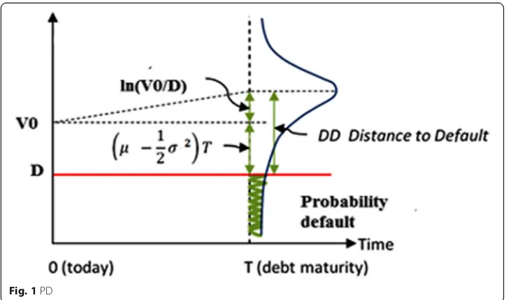
whereμ_V is expected rate of return of the firm’s asset and Dis the face value of a debt and expected growth of assets is equal toðμ_V−σV₂2Þ.

The numerator of Eq. (7) is really the distance to default; it demonstrates the distance between expected assets andDas appeared in Fig.1. It tends to be figured as a whole of initial distance and growth of that distance within the period T. Equation (7) is the distance to default in wording as a multiplier of standard deviation. The distance to de-fault is characterized as how much a firm is far off from the dede-fault point. Subsequent to evaluating the distance to default, we can create and gauge the probability of default. The PD under the risk neutral measure as per the Black Scholes Merton model is given by:

Probability default¼Nð−d2Þ ¼N −

ln V

D þ μV−

σV2 2 T σV ffiffiffiffi T p 0 B B @ 1 C C

A ð8Þ

or

Probability of default = 1−N(d2), see references (Hull 2009; Valverde 2015; Dar and Anuradha2017; Merton1974)

Equation (8) is the probability of default that is it is distance between the value of the firm and the value of the debt (V/D) adjusted for the expected growth related to asset volatilityðμ_V−σV2

2 Þ.

Equation (8) is the PD with three unknownsV,σV, andμV. To appraise the probability

as per Eq. (7), the authors have to locate the above three unknowns. The value of the firm V is equal to the sum of the debt and the equity of the firm, so the debt D is known and we need to find equity E.

The equity valueEis a continuous time stochastic process that is Weiner process.

E¼μ_EEdtþσEEdZ ð9Þ

where dZ is the continuous time stochastic process, μE is the expected continuously

compounded return onE, andσEis the volatility of the equity value. By Ito’s lemma,

dfð Þ:

dx YtdZtþ dfð Þ:

dt þAt dfð Þ:

dx þ0:5 d2fð Þ:

dx2 Yt

2

dt

We can represent the process for equity E as:

dE¼σVV dE dVdZþ

dE dtþμVV

dE

dVþ0:5ðσVVÞ

2d2E

dV2

dt ð10Þ

As per the diffusion terms Eqs. (9) and (10) is equal, so we can write the relation between the two equations as:

σEE¼σVV dE

dV ¼σVN dð Þ1 ð11Þ

Equations (5) and (11) having two unknowns one isσVand another isV. We can

eas-ily estimate the two parameters by solving Eqs. (5) and (11). After finding theVandσV,

we need to find the return of the asset that isμV.

Returm¼today

0_{s price−yestarday}0_{s price}

yestarday0s price

So,

μV ¼

Vt−Vt−1

Vt−1 ð

12Þ

In most cases, the return is negative, as was mentioned in Hillegeist et al. (2004). Based on the accounting data, there are several problems when modeling probability of default, he argues. The expected return cannot be a negative. Here, assume that the ex-pected growth is equal to the risk-free rate of interest.

Use all the known parameters that isE, r,D, T andσEto estimate the three unknown

parameters V,σV, andμV.

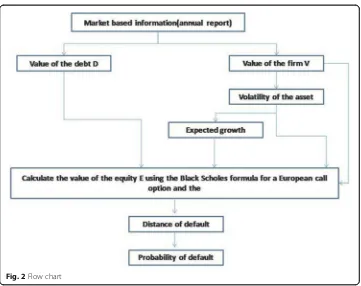
As per the above calculation, draw a model for probability of default as shown in Fig.2:

Result and discussion

This study has taken the secondary data of all the firms for 5 years starting from March 2012 to March 2016. The BSM-CO has been used to estimate the PD of all firms using BSM models:

To estimate the PD, this study used parameters like:

1. Firm value of assets,V(total equity + debt) 2. Value of a debt,D

3. Volatility of an asset,σ 4. Rate of return,μV. 5. Time period,T

Result

The PD of Jammu and Kashmir bank is 26.88% in year 2012 as shown in Table1, which suggests that the likelihood of Jammu and Kashmir (JK) Bank to be a default in the year 2012 is 26.88% that is 26.88% obligations that Jammu and Kashmir Bank has not paid.

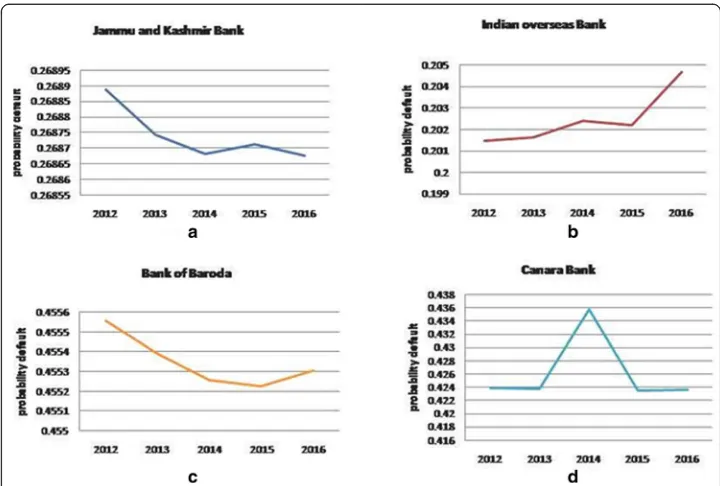
Figure3demonstrates the PD of the considerable number of firms. Each firm is having the distinctive PD at various day and age. The inquiry is which organization is great that a speculator will give an advance to the firm? The appropriate response is straightforward; the firm which is having the less PD, e.g., a financial specialist ABC needs to give the ad-vance to one firm in 2013. The speculator ABC is having four firms where he can put; however, he will put in just one firm. As shown in Table1, the PD of Jammu and Kashmir Bank, Indian Overseas Bank, Bank of Baroda, and Canara Bank is 26.88%, 20.148%, 45.55%, and 42.38%, respectively, in year 2012. Based on past data with respect to the four firms, the financial specialist will give advance to Indian Overseas Bank since it has less PD as shown in Table1.

Fig. 2Flow chart

Table 1PD of different firms using equation (8)

Year Jammu and Kashmir Bank Indian overseas Bank Bank of Baroda Canara Bank

2012 0.268888 0.20148 0.4555564 0.423839

2013 0.2687425 0.2016335 0.4553912 0.4237237

2014 0.268681897 0.202425 0.4552581 0.435759

2015 0.268711978 0.2022066 0.4552265 0.4234976

2016 0.268676859 0.2046978 0.4553076 0.4236178

Note:

•Taking total equity and value of debt from historical data of JK Bank •Firm value of assets = total equity + debt

Take a gander at Fig. 3, where the PD in all organizations’ increments or abate-ments is demonstrated. The Indian Overseas bank is enhancing according to our outcome. The bank of Baroda diminishes and after that it increments. The Jammu and Kashmir diminishes at all which is a decent sign, and the Canara Bank incre-ments first and after that it begins to diminish moreover. Presently, the authors will complete a speculation test on all the four firms to observe any contrast between the methods (Table 2).

One-way ANOVA for four independent samples

In order to determine whether there is any mean difference between the PD of the firms given in Table1. The authors compare thepvalues of all the mean values of pa-rameters with the significance level (α= 5%). Theαindicated that the risk of conclud-ing that the parameters are significantly different (Refer Table3).

In order to verify, we have two cases:

Fig. 3PD of all firmsaJammu and Kashmir BankbIndian overseas BankcBank of BarodadCanara Bank

Table 2Basic statistics

Data Summary Jammu and Kashmir Bank Indian overseas Bank Bank of Baroda Canara Bank Total

N 5 5 5 5 20

Sum 1.3437 1.0124 2.2767 2.1304 6.7633

Mean 0.2687 0.2025 0.4553 0.4261 0.3382

Sumsq 0.3611 0.205 1.0367 0.9079 2.5107

SS 0 0 0 0.0001 0.2236

Variance 0 0 0 0 0.0118

St. dev. 0.0001 0.0013 0.0001 0.0054 0.1085

1. Ifpvalue >α(0.05), there is no mean difference (fail to reject the null hypothesis or accept the null hypothesis).

2. Ifpvalue≤α(0.05), there is mean difference (reject the null hypothesis).

Null hypothesis All means are equal

Alternative hypothesis Not all means are equal

Significance level α= 0.05

Equal variances were assumed for the analysis.

Factor information

Factor Levels Values

Factor 4 JK Bank, IOB, BOB, Canara Bank

The ANOVA is used to explain that the mean response between the firms varies or not. If there are no differences between the means of all the firms then the F value is around 1. If the F value is large, then there are mean difference between the firms.

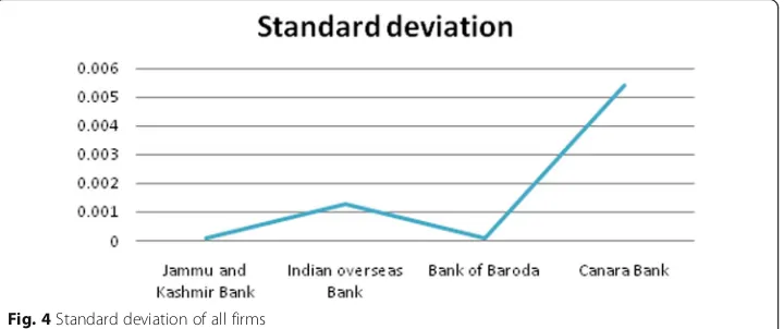
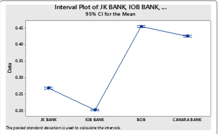
The standard deviation of all firms in several years gives the measurement of variance of probability of default (Fig.4).

ANOVA summary

A hypothesis is a test whether there is any such difference between the treatments based on the F ratio. It will ask whether the F ratio for the treatments is unusually high by comparing the F ratio to a kind of a standard distribution called an F distribution. Thepvalue for the treatments is the probability of getting such a high F ratio if all the treatments were really identical.

Table 3ANOVA

Source DF Adj SS Adj MS F value pvalue

Factor 3 0.223450 0.074483 9626.24 0.000

Error 16 0.000124 0.000008

Total 19 0.223574

The p value less that 0.005 indicates that there are differences between the treatments among the four firms. In other words, we have a strong evidence to reject the null hypothesis that the mean of PD score varies.

Tukey pairwise comparisons

It is a method that applies simultaneously to the set of pairwise comparisons

mi−mj

wheremis a mean.

Tukey’s method is used in ANOVA to create confidence intervals for all pairwise differences between factor-level means. This method is used in order to check whether there is any mean difference between the pairs of parameters. If the value zero lies in between the intervals, then there is no mean difference between the pairs.

Table 4 shows that all the factors have a different letters, group A consists Bank of Baroda (BOB), group B consists Canara Bank, group C consists JK Bank, and group D consists Indian Overseas Bank (IOB). All the firms do not share any letter, which indicates that BOB has a significantly higher mean of PD than others. But more PD means more risky. The IOB has lower PD which indicates that it is the best firm as compared to the others as shown in Fig.5.

Table 4Grouping information using the Tukey method and 95% confidence

Factor N Mean Grouping

BOB 5 0.455348 A

Canara Bank 5 0.42609 B

JK Bank 5 0.268740 C

IOB 5 0.202489 D

Note: Means that do not share a letter are significantly different

Note: Rank the firm from D to A, D indicates the best firm because less PD means better and that is why we have to choose the ranking from D to A.

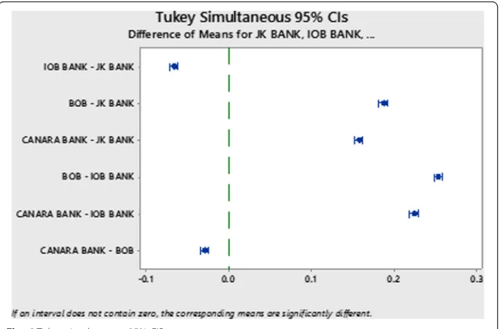
The results from Tukey simultaneous 95%CIs are (Table5):

a. All the pairs do not contain the value zero. The pairs consist a positive or negative value. The Tukey method states that“If the pair or a group contain zero value or the interval of the pair is between positive and negatives values that indicates the groups are not significantly different.”Table5and Fig.6show that all the pairs are not containing zero which means all are the firms are significantly different b. The 95% simultaneous confidence level indicates that you can be 95% sure that all

the confidence intervals have the right value

c. The 98.87% individual confidence level indicates that you can be 98.87% confident that every individual interval contains the right difference between the specific pair of group mean.

Table 5Tukey simultaneous tests for differences of means

Difference of levels Difference of means SE of Difference 95% CI T value AdjustedPvalue

IOB–JK Bank −0.06625 0.00176 (−0.07129,−0.06121) −37.66 0.000

BOB–JK Bank 0.18661 0.00176 (0.18157, 0.19165) 106.07 0.000

Canara Bank–JK Bank 0.15735 0.00176 (0.15231, 0.16239) 89.44 0.000

BOB–IOB 0.25286 0.00176 (0.24782, 0.25790) 143.73 0.000

Canara Bank–IOB 0.22360 0.00176 (0.21856, 0.22864) 127.10 0.000

Canara Bank–BOB −0.02926 0.00176 (−0.03430,−0.02422) −16.63 0.000

Note: Individual confidence level = 98.87%

Conclusion

The conclusion of this study is summarized below:

1. The solution ofdVtisVt¼V0eσZtþðμ−0:5σ

2_Þt

2. The researchers cannot decide the decision on the basis of overall standard deviation, better and best methods are to measure the distance to default and the PD for an investor to invest the money in any firm because the PD will give us the rate of default for a particular firm and the standard deviation of PD for several years gives the measurement of variance of the PD, and based on this, it is not helpful to calculate or decide which firm is best to invest as per the overall standard deviation of the probability of default

3. As per ANOVA, the authors reject the null hypothesis which indicates that there are differences between the mean among the four firms

4. The Tukey test clearly shows us that IOB is the better and BOB is the worst among the four firms as per rank. In other words, IOB is more significant than the other firms

5. It also indicates that the entire pairs do not contain zero values, which means that the firms are statistically significantly different from each other.

Abbreviations

ANOVA:Analysis of variance; BOB: Bank of Baroda; BSM-CO: Black-Scholes Model for European Call Option; CIs: Confidence intervals; IOB: Indian Overseas Bank; JK Bank: Jammu and Kashmir Bank; PD: Probability of default

Acknowledgements

We are grateful to Chief Editor Nezameddin Faghih and the reviewers for their insight comments and suggestions throughout the review process. Finally, we wish to thank our parents for encouraging us throughout the study. Corresponding Author: The completion of this study would have been not possible if not dependent on the steadfast support and the encouragement of my wife (Samiya Jan) for her motivational speeches. There are no other contributors.

Funding

Not applicable.

Availability of data and materials

The annual reports of firms from the year 2012–2016 and the data may not be correct but the procedure that I mentioned in this paper is defined well.

Authors’contributions

AAD designed the study. SQ collected the data from different firms in order to estimate the probability of default. AAD and NA analysed and interpreted the data. AAD drafted the manuscript. All the authors read and approved the final manuscript.

Competing interests

The authors declare that they have no competing interests.

Publisher’s Note

Springer Nature remains neutral with regard to jurisdictional claims in published maps and institutional affiliations.

Author details

1

Department of mathematics and Actuarial Science, B S Abdur Rahman Crescent Institute of Science and Technology, Chennai 48, India.2_{Department of Management Studies, B S Abdur Rahman Crescent Institute of Science and}

Technology, Chennai 48, India.3Department of Commerce, Desh Bhagat University, Fatehgarh Sahib, Punjab 01, India.

Received: 6 November 2018 Accepted: 4 February 2019

References

Bharath, S. T., & Shumway, T. (2008). Forecasting default with the Merton distance to default model.The Review of Financial Studies, 21(3), 1339–1369.https://doi.org/10.1093/rfs/hhn044.

Black, F., & Scholes, M. (1973). The pricing of options and corporate liabilities.Journal of Political Economy, 81(3), 637–654. Bohn, J. R. (2000). A survey of contingent-claims approaches to risky debt valuation. The Journal of Risk Finance, 1(3), 53–70.

https://doi.org/10.1108/eb043448.

Cangemi, B., De Servigny, A., & Friedman, C. (2003). Standard & poor’s credit risk tracker for private firms. Technical document.

https://www.researchgate.net/publication/265539863_Standard_Poor's_Credit_Risk_Tracker_for_Private_Firms_Technical_ Document

Crosbie, P., & Bohn, J. (2003).Modeling Default Risk. Moody’s KMV.

Dar, A. A., & Anuradha, N. (2017). Probability default in Black Scholes formula: a qualitative study.Journal of Business and Economic Development, 2(2), 99–106.https://doi.org/10.11648/j.jbed.20170202.15.

Delianedis, G., & Geske, R. L. (1999). Credit risk and risk neutral default probabilities: information about rating migrations and defaults.https://cloudfront.escholarship.org/dist/prd/content/qt7dm2d31p/qt7dm2d31p.pdf

Farmen, T., Fleten, S. E., Westgaard, S., & Wijst, S. (2004). Default Greeks under an objective probability measure. InNorwegian School of Science and Technology Management working paperhttp://citeseerx.ist.psu.edu/viewdoc/download?doi=10.1.1. 580.4756&rep=rep1&type=pdf.

Gonçalves, V. S., Martins, F. V., & Brandão, E. (2014). The determinants of credit default on start–up firms. econometric modeling using financial capital, human capital and industry dynamics variables (No. 534). FEP working papers.http:// wps.fep.up.pt/wps/wp534.pdf

Hillegeist, S. A., Keating, E. K., Cram, D. P., & Lundstedt, K. G. (2004). Assessing the probability of bankruptcy.Review of Accounting Studies, 9(1), 5–34.

Hull, J. C. (2009).Options, futures and other derivatives(7th ed.pp. 277–300). Pearson Education First Indian Reprint. Jessen, C., & Lando, D. (2015). Robustness of distance-to-default.Journal of Banking & Finance, 50(1), 493–505.https://doi.org/

10.2139/ssrn.2311228.

Kollar, B. (2014). Credit value at risk and options of its measurement. In2nd international conference on economics and social science (ICESS 2014), information engineering research institute, advances in education research(Vol. 61, pp. 143–147). Kollar, B., & Cisko,Š. (2014). Credit risk quantification with the use of CreditRisk+. InProceedings of ICMEBIS 2014 international

conference on management, education, business, and information science, Shanghai, China(pp. 43–46). Canada: EDUGait Press. Lehutova, K. (2011). Application of corporate metrics method to measure risk in logistics.Logistyka, 6.Instytut Logistyki i

Magazynowania.https://www.infona.pl/resource/bwmeta1.element.baztech-article-BPG8-0092-0010.

Merton, R. C. (1974). On the pricing of corporate debt: the risk structure of interest rates.The Journal of Finance, 29(2), 449– 470.https://doi.org/10.1111/j.1540-6261.1974.tb03058.x.

Saunders, A., & Allen, L. (2002).Credit risk measurement: new approaches to value at risk and other paradigms. New York: Wiley. Schuermann, T., & Hanson, S. G. (2004).Estimating probabilities of default (No. 190). Staff Report, Federal Reserve Bank of New

York.http://hdl.handle.net/10419/60699

Tudela, M., & Young, G. (2003).A Merton-model approach to assessing the default risk of UK public companies.https://doi.org/ 10.2139/ssrn.530642.

Valverde, R. (2015). An insurance model for the protection of corporations against the bankruptcy of suppliers by using the Black-Scholes-Merton model.IFAC-PapersOnLine, 48(3), 513–520.https://doi.org/10.1016/j.ifacol.2015.06.133.