OPTIMIZATION OF CNC TURNING PARAMETERS USING TAGUCHI METHOD AND GREY RELATIONAL ANALYSIS FOR HOT DIE STEEL H-13

(1)

Organized by C.O.E.T, Akola, ISTE, New Delhi & IWWA. Available Online at www.ijpret.com471

INTERNATIONAL JOURNAL OF PURE AND

APPLIED RESEARCH IN ENGINEERING AND

TECHNOLOGY

A PATH FOR HORIZING YOUR INNOVATIVE WORK

OPTIMIZATION OF CNC TURNING PARAMETERS USING TAGUCHI METHOD AND

GREY RELATIONAL ANALYSIS FOR HOT DIE STEEL H-13

MS. SHARDA RAMDAS NAYSE

Assistant Professor, Manav School of Engineering and Technology, Akola

Accepted Date: 07/09/2016; Published Date: 24/09/2016

Abstract: This work investigates the hard turning for cavity pin. Hot die steel (H-13)is an important material for various manufacturing industries mostly because of its high melting point, high degree of hardness and good wear resistance over a wide range of temperatures. It is used for drawing dies, blanking dies, forming dies, bushings etc. Even most CNC machine today have process control, but selecting and maintaining optimal setting is still an extremely difficult job which yet to be satisfactorily addressed. The objective was to optimize the process parameters of CNC turning of H-13 based on important technological characteristics. Also the effect of speed, feed and depth of cut individually studied on the final outcome to increase the material removal rate (MRR) and to decrease the tool tip temperature (T) and surface roughness (Ra), mathematical models will be established, relating the performance measures and input parameters by regression analysis. The working ranges of the parameters for subsequent design of experiment, based on Taguchi’s L9 Orthogonal Array (OA) designs have been selected. Statistical methods will be used to estimate relation between output parameters and input parameters like ANOVA and regression analysis. Optimization of process parameters is carried out by using grey relational analysis (GRA).

Keywords: CNC Turning Machining, Orthogonal Array, Signal-to-Noise ratio, Grey Relational Analysis

Corresponding Author:MS. SHARDA RAMDAS NAYSE

Co Author:

Access Online On:

www.ijpret.com

How to Cite This Article:

Sharda Ramdas Nayse, IJPRET, 2016; Volume 5 (2): 471-487 PAPER-QR CODE

SPECIAL ISSUE FOR

INTERNATIONAL CONFERENCE ON

“INNOVATIONS IN SCIENCE & TECHNOLOGY:

(2)

INTRODUCTION

The materials having high-tensile strength and resistance to wear and impact, which are frequently used in the aerospace and nuclear industries, are generally difficult to machine. High manganese steel is one of these materials. For the machining of high manganese steels, the cutting tool materials must be harder than the workpiece materials. These types of materials can be machined with sintered carbide tools and the speed steels with cobalt. Due to the high cost of changing and sharpening cutting tools, different machining methods are being used. Machining by softening the workpiece is a more effective method than strengthening the cutting tool. It is suggested that these materials should be machined by heating. The heating of the workpiece is not a new method for making easy the properties of the machinability of materials. For machining, it is necessary to choose the best heating method to heat the materials. Selecting the wrong heating method can induce undesirable structural changes in the workpiece and increases the machining cost. In the published works, there are different heating methods described which are used for heating the workpiece. Electrical resistance, plasma arc and other heating methods in hot machining have been used.

I. MATERIALS AND METHODS USED

A. Material and machine

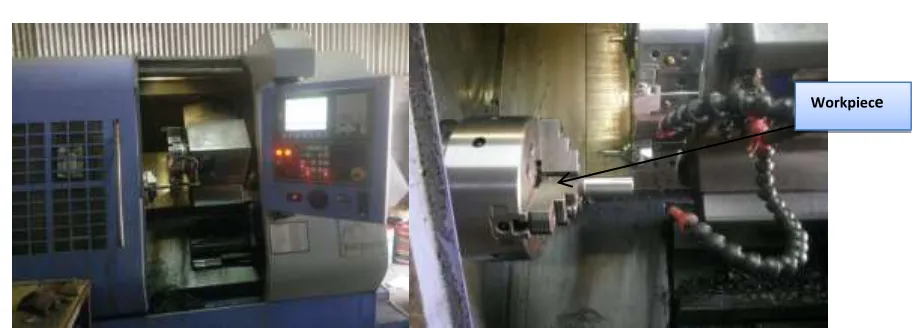
H-13 steel is commonly used for press tools and die components in automobile industries. EN-19 is a 5.25 % chromium – 1.25% molybdenum medium hardenability general purpose high tensile steel, generally supplied hardened and tempered in the tensile range of 1000 – 1200 0 F. H-13 steel is available with improved machinability, which greatly increases feeds and/or speeds, while also extending tool life without adversely affecting mechanical properties. Pre hardened and tempered H-13 can be further surface hardened by flame or induction hardening and by nitriding. Workpiece materials before machining and after machining are shown in Photograph 2.1.

(3)

a) b)

Photograph 2.1 Work piece before machining a) and after machining b)

Photograph 2.2 Cutting tool inserts

Table 2.2 Chemical composition of H-13

Element Content (wt %)

Chromium, Cr 4.75-5.50

Molybdenum, Mo 1.10-1.75

Silicon, Si 0.80-1.20

Vanadium, V 0.80-1.20

Carbon, C 0.32-0.45

Nickel, Ni 0.3

(4)

Manganese, Mn 0.20-0.50

Phosphorus, P 0.03

Sulfur, S 0.03

Table 2.2 Mechanical Properties of H-13

Properties Metric

Tensile strength, ultimate (@20°C/68°F, varies with heat treatment) 1200 - 1590 MPa

Tensile strength, yield (@20°C/68°F, varies with heat treatment 1000 - 1380 MPa

Reduction of area (@20°C/68°F) 0.5

Modulus of elasticity (@20°C/68°F) 215 GPa

Poisson's ratio 0.27-0.30

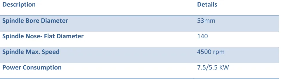
The turning operation is done on H-13 bar of Dia. 32 and 100 mm long bar. The steel bar is hardened to 48 ± 2 HRC using Induction hardening process. Induction hardening make outer layer of work piece hard and wear resistant but impact resisting property is still present inside the work material. Workpieces is hold between centre while turning and chamfered on both side to avoid cracking while induction hardening. Table 2.3 shows the mechanical properties.

Table 2.3 Mechanical Properties of H-13

Description Details

Spindle Bore Diameter 53mm

Spindle Nose- Flat Diameter 140

Spindle Max. Speed 4500 rpm

(5)

Model Macpower

Photograph 2.2: Setup for Hard Turning

The control parameters at three different levels and three different response parameters considered for multiple performance characteristics in this work are shown in Table 2.4.

Table 2.4 Response parameters and control parameters with their levels

Response Parameters Rise in tool tip temperature (˚C)

Material Removal Rate (mm3_/min.)

Surface Roughness (µm)

Control Parameters Levels

1 2 3

Speed (rpm) 1753 1984 2215

Feed (mm/rev) 0.02 0.03 0.04

Depth of Cut (mm) 0.7 1.2 1.7

(6)

B. Experimental Details

Design of Experiments (DOE) techniques enables designers to determine simultaneously the individual and interactive effects of many factors that could affect the output results in any design. DOE also provides a full insight of interaction between design elements; therefore, it helps turn any standard design into a robust one. Simply put, DOE helps to pin point the sensitive parts and sensitive areas in designs that cause problems in yield. Designers are then able to fix these problems and produce robust and higher yield designs prior going into production.

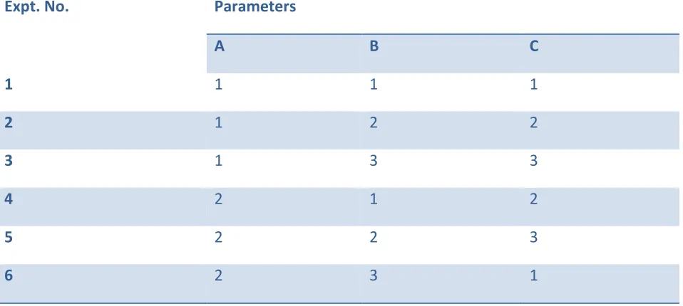
Design of experiment is an effective tool to design and conduct the experiments with minimum resources. Orthogonal Array is a statistical method of defining parameters that converts test areas into factors and levels. Test design using orthogonal array creates an efficient and concise test suite with fewer test cases without compromising test coverage. In this work, L9 Orthogonal Array design matrix is used to set the control parameters to evaluate the process performance. The Table 2.5 shows the design matrix used in this work.

A Cylindrical bar of H-13 (length 100 mm, diameter 32 mm) was used as workpiece to carry out experiments on CNC lathe by a PCBN insert as cutting tool without a coolant. The working ranges of the parameters for subsequent design of experiment, based on Taguchi’s L9 Orthogonal Array (OA) designs have been selected.

Table 2.5 Design Matrix of L9 Orthogonal Array

Expt. No. Parameters

A B C

1 1 1 1

2 1 2 2

3 1 3 3

4 2 1 2

5 2 2 3

(7)

7 3 1 3

8 3 2 1

9 3 3 2

C. Response parameters

The machining performance of the turning process can be evaluated by the material removal rate, temperature of tool tip. The accuracy of the machine part can be evaluated by surface roughness.

1) Material Removal Rate

The MRR for each run is calculated by weight difference of specimen before and after the machining.

Where, W1= weight of specimen before machining

W2= weight of specimen after machining

Tm= machining time

2) Tool tip temperature

Measurement of % Rise in cutting tool tip temperature at the chip interface (%RT)

Where, Tf = Final temperature of the cutting tool tip at the chip interface in °C

Ti = Initial temperature of the cutting tool tip at the chip interface in °C

(8)

Photograph 2.3: Equipment for tool tip temperature measurement

3) Surface roughness

Whenever two machined surfaces come in contact with one another the quality of the mating parts plays an important role in the performance and wear of the mating parts. Each of the roughness parameters is calculated using a formula for describing the surface. There are many different roughness parameters in use, but Ra is the most common. Other common parameters include Rz, Rq, and Rsk. Some parameters are used only in certain industries or within certain countries. For example, the Rk family of parameters is used mainly for cylinder bore linings. Since these parameters reduce all of the information in a profile to a single number, great care must be taken in applying and interpreting them. Small changes in how the raw profile data is filtered, how the mean line is calculated, and the physics of the measurement can greatly affect the calculated parameter. By convention every 2D roughness parameter is a capital R followed by additional characters in the subscript. The subscript identifies the formula that was used, and the R means that the formula was applied to a 2D roughness profile. Different capital letters imply that the formula was applied to a different profile. For example, Ra is the arithmetic average of the roughness profile.

(9)

Photograph 2.4: Surface roughness measuring instrument

II. ANALYSIS OF EXPERIMENTS

The experiments were conducted based on varying the process parameters, which affect the machining process to obtain the required quality characteristics. Quality characteristics are the response values or output values expected out of the experiments. There are 64 such quality characteristics. The most commonly used are:

1) Larger the better

2) Smaller the better

3) Nominal the best

4) Classified attribute

5) Signed target

(10)

A. Experimental Results

Table 3.1: Experimental Results

Expt. No.

Input Parameters Response

Speed (RPM) Feed (mm/rev) DOC (mm) MRR (gm/sec)

%RTTT (°C) Surface

Roughness Ra (µm)

1 1753 0.02 0.7 0.24 20.40 1.07

2 1753 0.03 1.2 0.79 23.23 1.62

3 1753 0.04 1.7 1.65 75.98 2.12

4 1984 0.02 1.2 0.27 17.44 1.09

5 1984 0.03 1.7 1.34 27.64 0.66

6 1984 0.04 0.7 0.62 23.82 0.71

7 2215 0.02 1.7 0.90 21.94 0.44

8 2215 0.03 0.7 0.50 10.24 0.22

9 2215 0.04 1.2 1.37 26.63 0.32

B. Optimization using Grey Relational Analysis

Table 3.2 Signal-to-Noise ratios

Exp No Response values S/N ratios

MRR (gm/sec))

%RTTT (°C) Surface

Roughness Ra (µm)

MRR (dB) %RTT (dB) Ra (dB)

(11)

2 0.79 23.23 1.62 -2.0475 -27.3210 -4.1635

3 1.65 75.98 2.12 4.3497 -37.6140 -6.5267

4 0.27 17.44 1.09 -11.3727 -24.8309 -0.7086

5 1.34 27.64 0.66 2.5421 -28.8308 3.6553

6 0.62 23.82 0.71 -4.1522 -27.5388 3.0362

7 0.90 21.94 0.44 -0.9151 -26.8247 7.0817

8 0.50 10.24 0.22 -6.0206 -20.2060 19.1721

9 1.37 26.63 0.32 2.7344 -28.5074 15.7562

Table 3.3 Normalized Signal-to-Noise ratios

Exp.

No.

Speed (RPM)

Feed (mm/rev)

DOC (mm) Normalized S/N Ratios

MRR %RTTT Ra

1 1753 0.02 0.7 0.0000 0.8455 0.555263

2 1753 0.03 1.2 0.3901 0.8024 0.265789

3 1753 0.04 1.7 1.0000 0.0000 0.0000

4 1984 0.02 1.2 0.0213 0.8905 0.544737

5 1984 0.03 1.7 0.7801 0.7353 0.770263

6 1984 0.04 0.7 0.2695 0.7934 0.744737

7 2215 0.02 1.7 0.4681 0.8220 0.882895

8 2215 0.03 0.7 0.1844 1.0000 11.0000

(12)

Table 3.4 Deviation sequences

Exp.

No.

Speed (RPM)

DOC (mm) Deviation Sequences

1 1753 0.02 0.7 1.0000 0.1545 0.444737

2 1753 0.03 1.2 0.6099 0.1976 0.734211

3 1753 0.04 1.7 0.0000 1.0000 1.0000

4 1984 0.02 1.2 0.9787 0.1095 0.455263

5 1984 0.03 1.7 0.2199 0.2647 0.229737

6 1984 0.04 0.7 0.7305 0.2066 0.255263

7 2215 0.02 1.7 0.5319 0.1780 0.117105

8 2215 0.03 0.7 0.8156 0.0000 0.0000

9 2215 0.04 1.2 0.1986 0.2493 0.052632

Table 3.5 Grey Relational Co-efficient

Exp.

No.

Speed (RPM)

DOC (mm) Grey Relational Coefficient

1 1753 0.02 0.7 0.3333 0.7639 0.529248

2 1753 0.03 1.2 0.4505 0.7167 0.405117

3 1753 0.04 1.7 1.0000 0.3333 0.333333

4 1984 0.02 1.2 0.3381 0.8203 0.523416

5 1984 0.03 1.7 0.6946 0.6539 0.685179

(13)

7 2215 0.02 1.7 0.4845 0.7375 0.810235

8 2215 0.03 0.7 0.3801 1.0000 1.0000

9 2215 0.04 1.2 0.7157 0.6673 0.904762

Table 3.6 Grey Relational Grade

Exp.

No.

Speed (RPM) Feed (mm/rev) DOC (mm) Grey

Relational

Grade

Rank

1 1753 0.02 0.7 0.542156 8

2 1753 0.03 1.2 0.524114 9

3 1753 0.04 1.7 0.555556 7

4 1984 0.02 1.2 0.56062 6

5 1984 0.03 1.7 0.677876 3

6 1984 0.04 0.7 0.592001 5

7 2215 0.02 1.7 0.677421 4

8 2215 0.03 0.7 0.793351 1

(14)

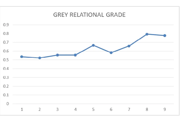
Organized by C.O.E.T, Akola, ISTE, New Delhi & IWWA. Available Online at www.ijpret.com484 Graph 3.1: Scatter plot of GRG Vs order of experiment

It is last step to determine the Optimal Factor and its Level Combination. The Graph 3.1 shows the Grey relational grades for maximum MRR, minimum %RTTT and minimum Ra. Since the experimental design is orthogonal, it is possible to separate out the effect of each machining parameter on the grey relational grade at different levels. For example, the mean of the grey relational grade for the speed at levels 1, 2 and 3 can be calculated by averaging the grey relational grade for the experiments 1 to 3, 4 to 6, and 7 to 9 respectively. The mean of the grey relational grade for each level of the machining parameters is summarized and shown the mean of the grey relational grade for each level of the machining parameters.

Table 3.7: The Main Effects of the Factors on the Grey Relational Grade

Symbols parameters Grey Relational Grade Main effect Rank

Level-1 Level-2 Level-3

A SPEED 0.540609 0.6102 0.7445 0.2038 1

B FEED 0.5934 0.6651 0.636716 0.0717 2

C DOC 0.6425 0.6158 0.636951 0.0267 3

(15)

Organized by C.O.E.T, Akola, ISTE, New Delhi & IWWA. Available Online at www.ijpret.com485 performance characteristics still needs to be known, so that the optimal combinations of the machining parameter levels can be determined more accurately. From Table 3.7 the optimal parameter combination can be determined as A3 (Speed, 2215 rpm), B2 (Feed, 0.03 mm/rev) and C1 (DOC, 0.7 mm)

(a) (b) (c)

Graph 4.5: Grey relational grades for each level of parameters for (a) Speed (b) Feed

(c) Depth of cut

C. Confirmation Test

The purpose of the confirmation experiment is to validate the conclusions drawn during the analysis phase. After determining the optimum level of process parameters, a new experiment is designed and conducted with optimum levels of parameters obtained.

Confirmatory experiments were performed using the optimum values and it was found that experimental response values were close enough to predicted values. These values and percentage error between actual and predicted values of the responses are given in Table 3.8. The percentage error between the actual and predicted values of the responses falls below 5%, which shows that the optimized value of process parameters obtained is good enough for achieving the target set during the experiment. The comparison again shows the good agreement between the predicted and the experimental values.

Table 3.8: Confirmation results

Predicted Experimental % Error

(16)

% RTTT (Degree

Celsius)

9.55 10.02 4.69

Ra (µm) 0.22 0.23 4.3

Confirmatory experiments were performed using the optimum values and it was found that experimental response values were close enough to predicted values. These values and percentage error between actual and predicted values of the responses are given in Table 3.8. The percentage error between the actual and predicted values of the responses falls below 5%, which shows that the optimized value of process parameters obtained is good enough for achieving the target set during the experiment. The comparison again shows the good agreement between the predicted and the experimental values.

III. CONCLUSIONS

Taguchi’s Signal – to – Noise ratio and Grey Relational Analysis were applied in this work to improve the multi-response characteristics such as MRR (Material Removal Rate), %RTTT (Rise in Tool Tip Temperature) and Surface Roughness of hot die steel H-13 during CNC process. The conclusions of this work are summarized as follows:

 The optimal parameters combination was determined as A3B2C1 i.e. A3 (Speed, 2215 rpm), B2 (Feed, 0.03 mm/rev) and C1 (DOC, 0.7 mm).

 The predicted results were checked with experimental results and a good agreement was found.

 This work demonstrates the method of using Taguchi methods for optimizing the CNC turning parameters for multiple response characteristics.

REFERENCES

1. Tosun N. Ozler E. L, “Optimization for hot turning operations with multiple performance characteristics”, International Journal of Advanced Manufacturing Technology, (2004) 23: 777– 782 DOI 10.1007/s00170-003-1672-4.

(17)

Organized by C.O.E.T, Akola, ISTE, New Delhi & IWWA. Available Online at www.ijpret.com487 3. Thamizhmanii S. Saparudin S. and Hasan S., (2007), “Analysis of Surface Roughness by Using Taguchi Method”, Achievements in Materials and Manufacturing Engineering, Volume 20, Issue 1-2, pp. 503-505.

4. Wang M. Y. and Lan T. S., (2008), “Parametric Optimization on Multi-Objective Precision Turning Using Grey Relational Analysis”. Information Technology Journal, Volume 7, pp.1072-1076.

5. Raghuraman S, Thiruppathi K, Panneerselvam T, Santosh S, “optimization of EDM parameters using taguchi method and grey relational analysis for mild steel is 2026”, International Journal of Innovative Research in Science, Engineering and Technology Vol. 2, Issue 7, July 2013.

6. G. Rajyalakshmi, Dr. P. Venkata Ramaiah “Simulation, Modeling and Optimization of Process parameters of Wire EDM using Taguchi –Grey Relational Analysis”, IJAIR ISSN: 2278-7844.

7. Douglas C. Montgomery “Design and Analysis of Experiments” Wiley, Singapore, 5th Edition 1996, 11-19,170-200.