1- INTRODUCTION
Networked control system (NCS) is a feedback control architecture wherein the sensors, controllers, and actuators are connected via a communication network. The advantages of NCSs such as low cost, simple installation, and maintenance have broadened their usage in many real-world applications from multi-agent to distributed control systems. However, the presence of communication links in the control loop makes analysis and design of NCSs challenging compared to the traditional point-to- point structures [1-3]. Main issues originate from data latency and dropout in the information exchange among system components through the communication medium.
Most of analyses and the design methods for NCSs rely on the Lyapunov-Krasovskii Theorem [4]. H∞ techniques for NCSs with data delay and loss were developed in [5-7]. In [5], on the basis of the appropriate Lyapunov–Krasovskii functional, the H∞ stabilization conditions were derived for NCSs with norm-bounded parameter uncertainty in the presence of both delay and dropout. In [6], latency and loss of data were modeled by a random variable with Bernoulli distribution and controller design conditions were extracted; however, the presented approach is not applicable to design NCSs with long delays. In [7], a linear Markov chain was employed to model data loss, and H∞ controller was designed for NCSs in which the upper bound of the data dropout is one sampling time.
In order to handle data latency and dropout in NCSs, state observer was utilized in [8-13]. In [8], the problem of designing an observer-based predictive controller for NCSs was investigated in two different cases without considering any delay in the forward channel. In the first case, a predictive observer located on the side of the plant estimates the states Corresponding author; Email: [email protected]
of the system; then, the estimated states are sent through a communication channel to the controller. In the second case, the measured outputs experience network delay before arriving at the predictive observer and the predicted states are used in the controller. In [9], a H∞ observer for switched linear systems with time-varying delay and exogenous disturbances was designed. By using the state observer, a controller is developed to stabilize a time-delay switched system, the design conditions are formulated in terms of delay-dependent LMIs.
Networked predictive controllers were proposed in [10, 11] where a sequence of future control predictions is generated on the side of the controller. An algorithm was employed at the actuator node to choose the appropriate control input according to the delay occurring in the forward channel. In [12, 13], the methods of [10, 11] were improved using a controller with switching gains which are chosen according to different values of the delay. In the mentioned approaches, a switched Lyapunov function which varies with respect to different delay values in the communication channels was used. However, the observer was located on the plant side, and, thus, delayed estimates of states are used in the controller; furthermore, the observer gain in [12, 13] is constant for different delay values.
In all the aforementioned methods, different delay values are supposed to have the same occurrence probabilities. In [14], using the information of delay occurrence probabilities in the synthesis procedure, a less conservative static controller was derived for NCSs; however, it was assumed that all the states of the controlled system are directly available.
In this paper, first, NCS is defined as a switched system; then, based on the notion of switched Lyapunov function, a new approach is introduced to design a robust stabilizing controller. The delay in the communication network varies randomly from zero up to a known upper bound; moreover, AUT J. Model. Simul., 50(1)(2018)23-30
DOI: 10.22060/miscj.2017.12188.5013
Design of Observer-Based H∞ Controller for Robust Stabilization of Networked
Systems Using Switched Lyapunov Functions
A. Farnam1, R. Mahboobi Esfanjani1,2*1 SYSTEMS Research Group, Ghent University, Ghent, Belgium
2 Department of Electrical Engineering, Sahand University of Technology, Tabriz, Iran
ABSTRACT: In this paper, a H∞ controller is synthesized for networked systems subject to random transmission delays with known upper bound and different occurrence probabilities in both feedback (sensor to controller) and forward (controller to actuator) channels. A remote observer is employed to improve the performance of the system by computing non-delayed estimates of the states. The closed-loop system is described in the framework of switched systems; then, a switched Lyapunov function is utilized to obtain conditions to determine the gains of the observer and the controller such that robust asymptotic stability of the system is assured. Two illustrative examples are presented to demonstrate the real-world applicability and superiority of the proposed approach compared to rival ones in the literatue.
Review History:
Received: 22 November 2016 Revised: 27 May 2017
Accepted: 28 May 2017 Available Online: 25 July 2017
Keywords:
Networked control system
H∞ controller
State observer
Random delays
information about the probability distribution of varying delay is known. Differently from [12, 13], according to each value of delay in the forward and feedback links, a quadratic term is incorporated in the energy function. Furthermore, unlike [12, 13], in a more practical configuration, the observer is located in the side of the remote controller. Thus, the non-delayed estimates of the states can be used in the controller to compute the control effort. Moreover, as in [14], the occurrence probabilities of the delay values are taken into account to reduce conservatism of the design sufficient conditions. The controller and observer gains are determined by solving a set of computationally tractable linear matrix inequalities which can be derived with utilizing switched energy function. Robust stabilization of NCSs is ensured with the desired disturbance attenuation level
ã
. Simulation results demonstrate that the maximum allowable delay bound is increased by the proposed scheme compared to state-of-the-art.This paper is organized as follows. The problem is explained in section II. Section III presents the main results of the paper wherein procedures are presented to determine controller and observer gains, maximum allowable delays in forward and feedback channels, and minimum disturbance attenuation level. In section IV, two numerical examples are given to illustrate the applicability and efficiency of the proposed method. Finally, Section V concludes the paper.
Notations: In this paper, R denotes real numbers set. The
symbol * stands for the symmetric block in the symmetric matrices. I is identity matrix with appropriate dimensions. The notation P 0> , (P 0)≥ means that P is real, symmetry, and positive definite, (semi definite). Prob .
{}
means theoccurrence probability of the event. The superscript
T stands for matrix transpose. The operator col{ } constitutes a column vector composed of elements in the braces.l2
[
0,∞)
denotes the space of square summable infinite vector sequences over [0, ∞).2- Problem Formulation
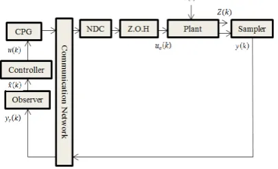
A typical NCS is shown in Fig. 1, wherein the controller is located far from the actuator and the sensor. The sensor is time-driven and the observer, controller, and actuator are all event-driven. In the considered network, all the data are lumped together into one packet and transmitted at the same time (single packet transmission), where the sent packets are time stamped. In the controller and actuator side, the new data packet is always used and the old ones are discarded; i.e. when an old data packet arrives, it is dealt with as a packet loss. It is assumed that the upper bounds of channel-induced delays in the both feedback and forward channels are known and indicated by N1 and N2.
Fig. 1. Structure of networked control system (NCS)
The output of Zero Order Hold (ZOH) is updated between sampling instances. Control prediction generator (CPG) on the side of the controller generates a sequence of future control actions. Furthermore, network delay compensator (NDC) close to ZOH applies the appropriate control action to the plant according to the value of delay in the forward channel.
The controlled plant is a linear time-invariant system and is described by the following discrete-time dynamical model:
(
1)
( )
c( )
( )
x k+ =Ax k +Bu k +E k
ω
( )
( )
y k =Cx k (1)
( )
( )
c( )
Z k =Fx k +Du k where, x k
( )
∈Rn,( )
mc
u k ∈R , Z k
( )
∈Rl, y k( )
∈Rpand
ω
( )
k ∈Rq are the state, control input, controlled output,measured output, and disturbance input belonging to l2
[
0,∞)
,respectively. A, B, E, C, F and D are the known and real matrices with appropriate dimensions. The pair (A, B) is controllable, and the pair (A, C) is observable.
The channel-induced delay in the forward channel is denoted by dk and assumed to take finite values from the set
{
0,1,2, ,… N1}
. To compensate the forward delay dk, CPG computes all the probable future control actions as follows:(
| k)
dkˆ(
k)
u k k d− =K x k d− (2) which are sent to NDC, wherein regarding the actual occurred
,
k
d an appropriate control action is taken to be applied to the plant:
(
| k)
dkˆ(
k)
u k k d− =K x k d− (3) where
k
d
K is the controller gain with an appropriate dimension and dk is the computed delay for the control action in the forward channel. The probabilities of induced delays in the forward channel are denoted as follows:
{
}
0Prob dk=0 =β ,
{
}
1Prob dk= =1 β ,
{
1}
1Prob dk = N =βN . (4)
As Fig. 1 depicts, the observer is located next to the controller. The equation of the observer is as follows::
(
)
( )
( )
(
( )
( )
)
ˆ 1 ˆ ˆc k c ˆc
x k+ =Ax k +Bu k +L y kτ −y k
( )
(
)
(
)
c k k
y k =y k−
τ
=Cx k−τ
, (5) where Lτk is the observer gain with an appropriate dimension, and τk is the network-induced delay in the feedback channel assumed to take values from the finite set,{
0,1, 2, , … N2}
. The occurrence probabilities of the network-induced delays in the feedback channels are as follows:{
}
0Prob τk =0 =α ,
{
}
1Prob τk = =1 α,
{
2}
2.Prob τk =N =αN (6)
The observer outputs and inputs, i.e. y kˆc
( )
and u kˆc( )
, are computed as follows:( )
( )
(
)
(
)
2
0 1 2
ˆc 1 N ˆ
y k =α C x k +αC x k− +…+ α C x k N−
(
)
2
0
N j j , j
C x k
α τ
=
=
∑
− (7)( )
( )
(
)
(
)
1 1
0 0 1 1 1
ˆc 1 N N
u k =β K x k +β K x k− +…+β K x k N−
1
(
)
0, N
i i i
i
K x k d
β
=
=
∑
− (8)with τ0=0, τ1= …1 , , τN2 =N2 and d0=0, d1= …1, , dN1=N1. Now, the models of the plant (1) and the observer (5) can be rewritten as
(
1)
( )
dkˆ(
k)
( )
x k+ =Ax k +BK x k d− +E k
ω
( )
( )
y k =Cx k
( )
( )
dkˆ(
k)
Z k =Fx k +DK x k d− (9)
(
)
( )
1 (
)
0
ˆ 1 ˆ B N i i i i
x k A x k
β
K x k d=
+ = +
∑
− +
(
)
2 (
)
0
k k N j j j j
L Cx kτ τ α L C x k τ = − − −
∑
In what follows, after defining new augmented state vector, the overall closed-loop system is formulated as a switched system. To this end, first, the binary stochastic variables
and j
α βi are defined as follows,
( )
1 , 0 k j j if k otherwise τ τ α = = ( )
1.
0
k i
i
if d d k
otherwise
β = =
It is supposed thatβi
( )
k and αj( )
k are independent Bernoulli distributed white sequences.Note that
( )
1 0 1, N i i k β = =∑
( )
{
i}
{
k i}
i.E β k =prob d =d =β (10)
( )
2 0 1, N j j k α = =∑
( )
{
j}
{
k j}
j .E α k = prob τ =τ = α (11) Hence, the closed-loop system (9) can be rewritten as follows
(
)
( )
1( )
(
)
0
1 N i i i
i
x k Ax k B β k K x k d
=
+ = +
∑
− +E kω( )
( )
( )
1( )
(
)
0
ˆ
N
i i i
i
Z k Fx k β k DK x k d
=
= +
∑
− (12)(
)
( )
1(
)
2( )
(
)
2(
)
0 0 0
ˆ 1 ˆ N i iˆ i N j j j N j j ˆ j
i j j
x k Ax k βBK x k d α k L Cx k τ α L Cx k τ
= = =
+ = +
∑
− +∑
− −∑
−(
)
( )
1(
)
2( )
(
)
2(
)
0 0 0
ˆ 1 ˆ N i iˆ i N j j j N j j ˆ j
i j j
x k Ax k βBK x k d α k L Cx k τ α L Cx k τ
= = =
+ = +
∑
− +∑
− −∑
−(
)
( )
1(
)
2( )
(
)
2(
)
0 0 0
ˆ 1 ˆ N i iˆ i N j j j N j j ˆ j
i j j
x k Ax k βBK x k d α k L Cx k τ α L Cx k τ
= = =
+ = +
∑
− +∑
− −∑
− .Regarding the theory of switched systems, the closed-loop system described in (12) is rewritten as
(
)
1 2( )
(
( )
( )
)
0 0
1 N N ij ij i j
x k k A x k E kω
= =
+ =
∑∑
Ψ +( )
1( ) ( )
( )
0 13 N
i i
i
Z k β k πx k
=
=
∑
(13)
where, Ψij
( ) { }
k ∈ 0,1 is the switching function which dependson the occurrence of two stochastic variables βi
( )
k and( )
j k
α .
( )
1 , , 0 k k ijif d i j k otherwise τ = = Ψ =
For instance, if the network-induced delays take values 1 in forward and feedback channels; then Ψ11
( )
k =1 and( )
0ij k
Ψ = for i≠1, 1j≠ . Aij and x k
( )
are defined in what follows: 1 2 3 4 i j ijA = ΛΛ ΛΛ
• Case 1: N1>N2
( )
{
( ) (
, 1 , ,)
(
2) ( ) (
, ˆ ,ˆ 1)
, ,ˆ(
2)
, ,ˆ(
1)
}
x k =col x k x k− … x k N− x k x k− … x k N− … x k N−
( )
{
( ) (
, 1 , ,)
(
2) ( ) (
, ˆ ,ˆ 1)
, ,ˆ(
2)
, ,ˆ(
1)
}
x k =col x k x k− … x k N− x k x k− … x k N− … x k N− and,
2 2 2 1 0 , 0
n N n
N n N n n
A I × × Λ = ( ) ( ) 1 2 1 2 1 üüüü , 0 i
n in i n N i n
N n N n
BK × × − × + Λ = ( ) ( ) 2 1 2 3 1
0 0
, 0
j
n jn j n N j n
N n N n
L C × × − × + Λ = 1 1 4 , 0 N n N n n
A I ϕ × Λ = with ( )
2 2 2 1
0 0L C 1 1L C 2 2L C NL CN 0n N N n
ϕ= −α α α …α × − +
1 1
0 0 1 1
β BK βBK … βNBKN
( )
2 1
0 0 0
i F l N n l in DKi l N i n
π = × × × −
( 1 2 1)
0N N n q
E E + + × =
• Case 2: N1<N2
( )
{( ) (
, 1 , ,)
(
2)
,x k =col x k x k− … x k N−
( ) (
)
(
1)
(
2)
, x k x kˆ ˆ − …1 , ,x k Nˆ − , ,… x k Nˆ − } and,
2 2 2 1 0 , 0
n N n
N n N n n
A I × × Λ = ( ) ( ) ( )
1 2 1
2 2
2
1
0 0 0
0 i
n in i n N i n n N N n
N n N n
BK × × − × − × + Λ = ( ) ( ) 2 2 2 3 1
0 0
, 0
j
n jn j n N j n
N n N n
L C × × − × + Λ = 2 2 4
, 0
N n N n n
A I ϕ × Λ = with, 2 2 0 0L C 1 1L C 2 2L C NL CN
ϕ= −α α α …α +
( )
1 1 2 1
0 0 1 1
i
π =F 0l N n l in× 2 0 × DKi 0l N i n×( 1−) 0l N N n×( 2− 1)
( 1 2 1)
0N N n q
E E + + × =
• Case 3: N1=N2=N
( )
{
( ) (
, 1 , ,)
(
) ( ) (
, ˆ ,ˆ 1 , ,)
ˆ(
)
}
x k =col x k x k− … x k N− x k x k− … x k N−
( )
{
( ) (
, 1 , ,)
(
) ( ) (
, ˆ ,ˆ 1 , ,)
ˆ(
)
}
x k =col x k x k− … x k N− x k x k− … x k N−
and, 1 0 , 0
n N n
N n Nn n
A I × × Λ = ( ) ( ) – 2 1 0 0 , 0 i
n in i n N i n
N n N n
BK × × × + Λ = ( ) ( ) – 3 1
0 0
, 0
j
n jn j n N j n
N n N n
L C × × × + Λ = 4 , 0
N n Nn n
A I ϕ × Λ = with,
ϕ = −
[
α0 0L C α1 1L C α2 2L C … αN NL C]
0 0 1 1
+ β BK βBK …βNBKN
( )
0 0 0
i F l N n l in DKi l N i n
π = × × × −
(2 1)
0 N n q
E E + × =
Remark 2. The novelty of the proposed structure for NCS is threefold. First, the observer is located nearby the controller, thus, unlike [12], the estimated states which are used in computation of the control signal do not include any delay; i.e. feedback link latency is compensated. Second, unlike [12, 13], the observer gain is switched with respect to the delay value in the feedback channel. Finally, the significant distinction is that different delay values in the forward and feedback channels have their own occurrence probabilities. It is a more realistic assumption compared to that made in [12, 13].
So far, the closed-loop NCS, which includes the introduced switching controller (2) and the observer (5), has been formulated as a linear switched system (13). In the next section, a systematic procedure is derived to determine the controller and observer gains. Before proceeding, some preliminaries are presented.
Definition 1. The closed-loop system (10) is said to be mean-square stable if for
ω
( )
k =0, there existε
>
0
andδ
∈( )
0,1 such that for all x( )
0 and xˆ( )
0 ∈Rn thefollowing inequality holds:
( )
( )
( )
( )
2 2 ˆ ˆ 0 . 0 kx k x
Ex k ≤εδ Ex
(14)
Definition 2. For a given real value γ >0, system (10)
has an H∞ disturbance attenuation level γ >0 under zero-initial condition if there exists a state feedback law u k
( )
such that for all nonzero ω( )
k , Ki and Lj, the following condition is satisfied,( )
{
2}
2{
( )
2}
( )
0 0
. 15
k k
E Z k E k
∞ ∞
γ ω
= =
<
∑
∑
(15)3- Design Method
In this section, two procedures are developed to determine the gains of the proposed controller and the observer given in (2) and (5), respectively. To this end, a novel criterion is introduced in Lemma 1 to check the stability and performance of the switched system (13).
Lemma 1: For a given scalar γ >0, the system (13)
with the known controller and observer gains is mean-square stable with H∞ disturbance attenuation level
γ
, if there exist symmetric positive definite matrices{
1}
, 0,1,2, , ij
P i∈ … N and j∈
{
0,1,2, ,… N2}
, such that (16)holds for all i n, ∈
{
0,1,2, ,… N1}
and ,j m∈{
0,1,2, ,… N2}
,2
0
*
T
T T
ij nm nm ij nm nm ij ij ij i i i
T nm nm
A P E
A P A P
E P E I
β π π
γ
Ψ − Ψ + Ψ
= <
Ψ −
Ω . (16)
where,
( )
{
}
, jij E ij k β αi
Ψ = Ψ =
{
0,1,2, , 1}
,{
0,1,2, , 2}
,i∈ … N j∈ … N
( )
{
}
Ψ =nm E Ψnm k = β αn m,
{
0,1,2, , 1}
,{
0,1,2, , 2}
,n∈ … N m∈ … N
Proof. Stochastic switched Lyapunov function is chosen as follows
( )
(
)
1 2( ) ( )
( ) ( )
0 0
, N N T 17
ij ij
i j
V x k k x k k P x k
= =
=
∑∑
Ψ (17) where Pij are symmetric positive definite matrices. The difference of V x k k(
( )
,)
along the trajectory of the switched system (13) is given by(
)
(
1 , 1)
(
( )
,)
üüüü
∆ = + + − =
(
) (
)
(
)
1 2
0 0
N N T 1 1 1
ij ij
i j
x k k P x k
= = + Ψ + +
∑∑
( ) ( )
( )
1 2 0 0N N T .
ij ij
i j
x k k P x k
= =
−
∑∑
ΨWithout a loss of generality, it can be assumed that
(
)
( )
Ψij k+ = Ψ1 ij k , thus the above relation can be rewritten as follows,
(
)
( )
(
)
1 2 0 0 1 1 N N T nm nm n mV x k k P x k
= =
∆ =
∑∑
+ Ψ +( ) ( )
( )
( )
1 2
0 0
N N T . 18
ij ij
i j
x k k P x k
= =
−
∑∑
Ψ (18)Note that in (18), Ψnm
( )
k can be equal to Ψij( )
k .To ensure the stability and the H∞ performance, simultaneously; the following inequality must hold
( ) ( )
( ) ( )
{
T 2 T}
0.E V Z k Z k∆ + −γ ω k ω k < (19) With regards to (13) and (18), the following relations are obtained:
( ) ( )
( ) ( )
{
T 2 T}
(
( )
( )
)
T.ij
E V Z k Z k∆ + −γ ω k ω k = A x k +E kω
( )
( )
(
)
( )
( )
. T
nm nmP A x kij E kω x k ij ijP x k
( )
( )
2( ) ( )
( )
( )
( )
( )
T
T T T
i i i
x k x k
x k β π πx k γ ω k ω k k k
ω ω
+ − =
Ω
Thus, the system (13) is H∞ stable, if (16) is satisfied. ■ Remark 3. Differently from [12, 13], the switched multiple Lyapunov function in (17) includes distinct quadratic terms corresponding to each delay value in the feedback and forward links. Moreover, represents the stochastic nature of the switching function which is helpful in derivation of robust stability measure.
Lemma 1 presents sufficient condition for stability analysis of the NCS. However, this condition is nonlinear with respect to the controller and observer gains. Hence, it cannot be used to obtain s and s, efficiently. In what follows, Lemma 1 is utilized to derive a systematic approach to compute the mentioned parameters by solving computationally amenable LMIs.
Theorem 1. the system (13) with controller and observer gains Ki and Lj is mean-square H∞ stable with a given disturbance attenuation level γ, If there exist symmetric positive definite matrices Pij, i∈
{
0,1,2, ,…N1}
and 0,1,2, ,j∈{
…N2}
, for all i n, ∈{
0,1,2, ,… N1}
and{
2}
,j m∈ 0,1,2, ,…N ,
(
)
2 0
* 0 0 0
* * 2
* * *
T T
ij ij ij nm i i
T nm
nm nm
i
P A
I E
P I I
β π γ
β
−Ψ Ψ
− Ψ <
Ψ −
−
. (20)
Proof. Utilizing the Schur complement, (16) can be modified as follows:
( )
21 0
* 0 0 0
* *
* * *
T T
ij ij ij nm i i
T nm
nm nm
i
P A
I E P
I
β π γ
β
−
−Ψ Ψ
− Ψ <
−Ψ
−
(21)
On the other hand,
(
1) (
01)
nm nm nm
I P P I P− − − − ≥ , is equivalent to
1 2
nm nm
P− P I
− ≤ − . (22) Combining (21) with (22) yields (20). ■
Instead of using (22), an alternative method to obtain LMI conditions from (21) is to replace 1
nm
P− with nm
W . The constraint P Wnm nm=I is imposed by minimizing the trace of
nm nm
P W . The result is summarized in Theorem 2.
Theorem 2. The system (13) is mean-square H∞ stable
with a given disturbance attenuation level γ if the controller and observer gains Ki and Lj are determined by solving the following optimization problem for all i n, ∈
{
0,1,2, ,… N1}
and , j m∈
{
0,1,2, ,… N2}
, with variable Pnm , Wnm , Ki and jL ,
Minimize Trace
[
P Wnm nm]
(23) Subject to:0 nm
nm
P I I W
≥
2 0
* 0 0
0
* *
* * *
T T
ij ij ij nm i i
T nm
nm nm
i
P A
I E W
I
β π γ
β
−Ψ Ψ
− Ψ <
−Ψ
−
Remark 4. The observer and controller gains can be obtained by LMI feasibility problem (22) or alternatively by solving minimization problem (23) which leads to less conservative result. The second approach it needs more offline computation compared to (22).
4- Simulation Results
Simulation results are presented to demonstrate the merits of the proposed approach. To solve the LMI problems in Theorems 1 and 2, the LMI Toolbox of Matlab® is utilized
[16].
In example 1, the results obtained by the proposed method are compared with the ones of [11] and [12]. Maximum allowable delay bound (MADB) which is the maximum delay value that retains the stability of the system is used for the evaluation of methods. Simulation results verify that conservativeness of the design conditions is notably decreased by the suggested scheme compared to the rival ones in [11] and [12]. Moreover, the time response of simulation outcomes is contrasted with the ones of [12].
Example 1. Consider the following system [12]: 1.01 0.271 0.4880
, 0.4820 0.1 0.24
0.0020 0.3681 0.7070
A
−
=
5 5
1 2 3 3 2 ,
4 3 1 5 4
B C
= − =
0.02 0 0.03
, 0.01 , 0.04 0.01 0.01
F= E= I
(23)
which is controlled over a network. For the same disturbance attenuation level γ =0.025, the obtained MADB by Theorem 2 is 10 while the MADBs attained by the methods of [11] and [12] are 3 and 6, respectively. Table 1 which summarizes the results obtained by different approaches shows the advantages of the proposed design method.
Table 1. MADBs from different approaches Method [11] [12] Proposed Method
MADB 3 6 10
Furthermore, a simulation scenario is executed by the proposed controller. It is assumed that data is transmitted over a network in which different delays have uniform occurrence probabilities with a maximum delay that is equal to 140 msec. Choosing sampling interval 35 msec yields delay upper bounds 4N1=N2= . Delay occurrence probabilities are assumed to be βi=0.2, α =j 0.2, for ,i j∈
{
0,1,2,3,4}
. The disturbance input is taken as follows( )
1 1 1[
1 1 1 , 1]
3, 3 T
T
k k
k k k k
ω
≤ <
= ≤
The controller and observer gains for desired disturbance attenuation level γ =0.02 computed by solving (23) are shown in the following:
0
0.0038 0.0122 0.0451 0.0154 0.0084 0.0552
K = − −− −
,
1
0.0014 0.0117 0.0221 0.0124 0.0087 0.0584
K = − − −
2
0.0075 0.0165 0.018 0.0112 0.0043 0.0245
K = −− − −
,
3
0.0098 0.0125 0.0138 0.0074 0.0075 0.0293
K = −− − −
4
0.0122 0.0113 0.0121 0.0067 0.0063 0.0341
K = −− − −
0
0.2831 0.3210 0.0092 0.112 0.1852 0.0395 L
−
= −
−
,
1
0.2232 0.2745 0.0073 0.0873 0.1962 0.0326 L
−
= −
−
2
0.1972 0.2531 0.0012 0.1234 0.2345 0.0274 L
−
=
−
,
3
0.1713 0.2146 0.0045 0.1324 0.2571 0.0215 L
−
=
−
4
0.1523 0.1826 0.0081 0.1401 0.2772 0.0198 L
−
=
−
Fig. 2-4 depict the outputs, control inputs and estimated states, respectively, with initial condition xT
( )
0 =[
0.1 0.1 0.1]
. Inthe proposed method, using variable observer gains and non-delayed estimated states lead to a remarkable improvement compared to [12].
Fig. 2. Outputs of the system in Example 1
Fig. 3. Control inputs of the system in Example 1.
Fig. 4. States of the observer in Example 1
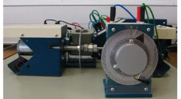
To demonstrate the real-world applicability of the proposed method, networked control of dc servo motor is simulated in example 2. The considered model belongs to a test rig comprising of a DC servo system depicted in Fig. 5 and a remote controller, connected via the Internet [13].
Fig. 5. DC servo plant controlled over the Internet [13]
Example 2: Consider the dynamic of DC servo motor as presented in [13]:
1 1.12 0.213 0.335
, 0
1 0 0
0
0 1 0
A B
−
= =
,
[
0.0541 0.1150 0.0001 ,]
C=
[
0.0500 0.1000 0.0005 ,]
D=
0.01
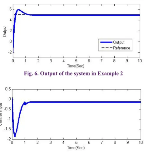
E= I (25) which is controlled over the Internet. It is assumed that the sampling period is 0.04s and the upper bounds of network-induced delays in feedback and forward channels are both 0.12s (maximum delay is considered to be 3 samples). Different delay values have their own occurrence probabilities as: α0=0.2, α1=0.2, α2=0.3, α3=0.3, β =0 0.3, β1=0.3, and β =2 0.4. Disturbance input is as (24). The controller and observer gains for disturbance attenuation level γ =0.095 are computed by solving (23) and are presented in the following.
[
]
0 0.0516 0.0085 0.0321
K = − − ,
[
]
1 0.0423 0.0112 0.0375
K = − − −
[
]
2 0.0401 0.0152 0.0346
K = − − −
[
]
T0 3.5122 3.2231 5.1315
L = ,
[
]
T1
L = 3.8891 3.5218 5.7182 ,
[
]
T2
L = 4.5108 2.8123 5.2821 ,
[
]
T3
Simulation results in Fig. 6 and Fig. 7 illustrate the efficiency of the proposed method. It should be noted that in [13] similar results are reported for maximum delay equal to 3.
Fig. 6. Output of the system in Example 2
Fig. 7. Control input of the system in Example 2 5- Conclusion
In this paper, in the framework of switched systems theory, a networked control system was designed. Here, the both feedback and forward channels suffer random delays with the known probability. To increase the maximum allowable delay bound, a remote observer was located on the side of the controller to import non-delayed estimates of states to the controller. Moreover, the both controller and observer gains can vary according to the value of delay. The less conservativeness of the proposed method was verified by simulations. Since the design criterion relies on the chosen switched Lyapunov function, by using more comprehensive energy function, less conservative sufficient conditions can be obtained in the future works.
References
[1] L. Zhang, H. Gao, O. Kaynak, Network-induced constraints in networked control systems-a survey, IEEE transactions on industrial informatics, 9(1) (2013) 403-416.
[2] J.P. Hespanha, P. Naghshtabrizi, Y. Xu, A survey of recent results in networked control systems, Proceedings of the IEEE, 95(1) (2007) 138-162.
[3] Y. Tipsuwan, M.-Y. Chow, Control methodologies in networked control systems, Control engineering practice, 11(10) (2003) 1099-1111.
[4] A. Farnam, R.M. Esfanjani, Improved stabilization
method for networked control systems with variable transmission delays and packet dropout, ISA transactions, 53(6) (2014) 1746-1753.
[5] S. Kim, P. Park, C. Jeong, Robust H∞ stabilisation of networked control systems with packet analyser, IET control theory & applications, 4(9) (2010) 1828-1837. [6] F. Yang, Z. Wang, Y. Hung, M. Gani, H∞ control for
networked systems with random communication delays, IEEE Transactions on Automatic Control, 51(3) (2006) 511-518.
[7] P. Seiler, R. Sengupta, An H∞ approach to networked control, IEEE Transactions on Automatic Control, 50(3) (2005) 356-364.
[8] H. Li, Z. Sun, H. Liu, M.Y. Chow, Predictive observer‐ based control for networked control systems with network‐induced delay and packet dropout, Asian journal of control, 10(6) (2008) 638-650.
[9] H. Liu, Y. Shen, X. Zhao, Delay-dependent observer-based H∞ finite-time control for switched systems with time-varying delay, Nonlinear Analysis: Hybrid Systems, 6(3) (2012) 885-898.
[10] G.-P. Liu, Y. Xia, J. Chen, D. Rees, W. Hu, Networked predictive control of systems with random network delays in both forward and feedback channels, IEEE Transactions on Industrial Electronics, 54(3) (2007) 1282-1297.
[11] G.-P. Liu, Y. Xia, D. Rees, W. Hu, Design and stability criteria of networked predictive control systems with random network delay in the feedback channel, IEEE Transactions on Systems, Man, and Cybernetics, Part C (Applications and Reviews), 37(2) (2007) 173-184. [12] R. Wang, B. Wang, G.-P. Liu, W. Wang, D. Rees, H∞
controller design for networked predictive control systems based on the average dwell-time approach, IEEE Transactions on Circuits and Systems II: Express Briefs, 57(4) (2010) 310-314.
[13] R. Wang, G.-P. Liu, W. Wang, D. Rees, Y.-B. Zhao, H∞ Control for Networked Predictive Control Systems Based on the Switched Lyapunov Function Method, IEEE transactions on industrial electronics, 57(10) (2010) 3565-3571.
[14] H. Gao, X. Meng, T. Chen, Stabilization of networked control systems with a new delay characterization, IEEE Transactions on Automatic Control, 53(9) (2008) 2142-2148.
[15] C. Peng, D. Yue, E. Tian, Z. Gu, A delay distribution based stability analysis and synthesis approach for networked control systems, Journal of the Franklin Institute, 346(4) (2009) 349-365.
[16] P. Gahinet, A. Nemirovski, A. Laub, M. Chilali, LMI Control Toolbox User’s Guide. Natick, The MathWorks, Inc. P. Gahinet, (1995).
Please cite this article using: