*Corr. Author’s Address: Iskra ISD-Strugarstvo d.o.o., 110
Application of Genetic Algorithm into Multicriteria Batch
Manufacturing Scheduling
Aleš Slak1,* - Jože Tavčar2 - Jože Duhovnik3 1Iskra ISD-Strugarstvo d.o.o., Slovenia
2 Iskra Mehanizmi, Slovenia
3University of Ljubljana, Faculty of Mechanical Engineering, Slovenia
Technical innovations in the area of manufacturing logistics are introduced partially and thus fail to realize their full potential. In order to optimise the efficiency of turning manufacturing processes, the production planning and scheduling, cutting tools and material flow process, manufacturing capacities have been analysed. All data from production operations, quantities and the, duration of operations are now kept in the ERP system. It provided the necessary condition for the establishment of a robust planning model, which includes stock control of material and cutting tools. An update was required for the whole lifecycle of products and means of work. The article presents information and an algorithm for a dynamic scheduling model, based on a genetic algorithm. The orders on the machines are scheduled on the basis of a genetic algorithm, according to the target function criteria. The algorithm provides a satisfactory, almost ideal solution, which is good enough for implementation in practice. With the GA the machine utilization increased, throughput time was reduced and costs and delivery delays improved. The presented model of GA also allows further optimisation of manufacturing plans and the machines layout.
©2011 Journal of Mechanical Engineering. All rights reserved.
Keywords: genetic algorithm, multicriteria scheduling, batch production, target function
0 INTRODUCTION
In the traditional approach, planning and scheduling are two separate and successive
operations. The production planning phase mostly
includes the physical aspect of planning, where a product range, production quantities, machines,
tools, material and accessories are selected. The
emphasis in the second, scheduling phase, is on the
time aspect. The plan is the basis for determining
the sequence of operations across available machines in a way that provides maximum machine utilisation and timely manufacturing. Differences between planning and scheduling criteria often lead to conflict situations or even opposition between respective goals.
Master production schedule (MPS)
and capacity requirement planning (CRP) in
the environment of manufacturing resources
planning (MRPII) are the most frequently applied traditional methods in practice. This system is
characterised by a hierarchical approach from top to bottom. Goals and restrictions at the lower level are determined by the results at the higher level. Such a planning method rarely takes account of
the scheduling problem. Separate treatment of planning and scheduling often results in plans
having to be manually modified. This leads
to significant rearrangement costs and supply delays. Nowadays, such planning does not provide efficient business operations as customers and the market require flexibility and quick response.
The solution for such problems is the
integration of the planning and scheduling
processes. The article presents a solution on a
case study of planning and scheduling in the batch production. Presented is a planning model and its advantages, compared to the existing method of work. A genetic algorithm was used
to optimise scheduling. The updated process
planning improved the efficiency of production and reliability of supplies.
1 LITERATURE REVIEW
The change of planning was triggered by
methods. Here, individual steps of the traditional approach are merged in a way that allows
automatic transition. Tasič et al. [2] presented
advanced scheduling methods, such as priority rules, useful also for sophisticated systems.
Computer Aided Process Planning (CAPP) has been recognised to play a key role in Computer Integrated Manufacturing (CIM) [3].
Traditionally, nearly all computer aided process
planning (CAPP) supposes that manufacturing is of secondary importance and that the workshop
has unlimited resources. This triggers unrealistic
plans that are unworkable in the manufacturing process.
Planning and scheduling functions often have opposing goals, which makes their separate
treatment less efficient. The other deficiency of
separate treatment is not taking account of the
dynamic manufacturing environment. The time
delay between process planning and the actual beginning of the plan can cause the plan to become unworkable. Fixed plans lead to bottleneck
situations. Research has shown that as many as 20
to 30% of all plans have to be modified in order to be adjusted to the dynamic manufacturing environment.
Integration between the planning and scheduling process is, therefore, vital as this is the only way to create more realistic plans and schedules. Only this will result in real CIM [4].
The integration creates a single space for solutions
and provides the basis for efficient integrated solutions that are in the interests of both, planning
and scheduling [5]. This contributes to an
improved efficiency of manufacturing resources, shorter throughput times, scheduling times and
shorter delays. The integration of planning and
scheduling is much more complex and more difficult to achieve in practice. Kumar et al. [6], suggested introducing on-line scheduling in a CAPP system where real time status of the shop floor is crucial and dynamic feedback is required for scheduling.
Larsen [7] and Alting [3] arranged different approaches to integrated process planning into
three types; The concept of non-linear process
planning (NLPP) or flexible process planning, closed loop process planning (CLPP) and distributed process planning (DPP).
The CLPP approach involves generating
plans by means of a dynamic feedback from the shop floor. It is better than NLPP since plans are generated with a view to realistic conditions in the
manufacturing environment. With this method, the
realistic conditions are vital and the feedback is important for the scheduling process.
DPP performs process planning simultaneously with the scheduling of manufacturing. Process planning is divided
into two phases. The first phase is the initial
phase where product requirements are analysed
according to its shape, tools, machines etc. When
all the requirements are satisfied, the second phase or final planning begins. During this phase, the required manufacturing resources and the
available resources are matched. The flexibility of
this approach increases if the required resources are given as alternatives. Examples of such an
approach are Wang and Shen [8] and the IPPM
system by Zhang [9], followed by IPPS by Huang et al. [4].
Matching individual planning models has shown that DPP is the best approach. However, it still requires high performance hardware and software. NLPP involves alternative plans, which allows better scheduling flexibility. Such a method can be introduced in enterprises without the need for their reorganisation, compared to DPP and CLPP that would require reorganisation
of the planning and scheduling departments. This
is due to CLPP and DPP requiring the merging of different separate processes within an enterprise.
Several researchers merged individual approaches in order to remove the deficiencies and come up with optimum plans. Gao et al. [10] presented an integrated process planning and scheduling model, based on taking the advantages of NLPP (alternative plans) and DPP (hierarchical
approach) models. Their model is based on the
principles of concurrent engineering, where computer-aided planning and scheduling are performed simultaneously.
The concept of non-linear process planning
is typical of integrated process planning and scheduling (IPPS). Usher and Fernandes [11]
presented the PARIS system, which is designed
improved hybrid genetic algorithm (HGA). To
improve the results, they also used heuristic rules,
i.e. the shortest processing time (SPT) and the longest processing time (LPT). Lee and Kim [22]
suggested simulation with a genetic algorithm, linked with a simulation module that calculates the success rate of planning, based on combinations
between process plans. Total production time and
delivery date were used as target functions. Gao et al. [10] suggest the use of a modified genetic algorithm where each function (process planning and scheduling) was given a different chromosome representation. Minimum throughput time of all products was used as the target function. For the integrated model a mathematical model, solved with genetic algorithms was introduced [23]. Lestan et al. [24] developed a simple genetic algorithm for a job-shop problem. Makespan as a target function was used and the solution was found without the help of heuristic rules.
The article describes a new approach with
GA in the batch production. Separate functions, production planning and scheduling are put together in one system. A planning model which comprehensively covers production planning has been developed. Constructing the model has shown that planning should also include material and tool purchases as well as product sales.
This model has served as a basis of determining
a satisfactory plan with genetic algorithms. Several target functions and criteria are present
in the optimisation procedure. This has improved
productivity, utilisation of machines and delivery times. Presented are also experimental results and a comparison with other authors is given.
2 PROBLEM DESCRIPTION: PLANNING AND SCHEDULING IN BATCH
PRODUCTION
Planning and scheduling of products in the production of turned parts are complex problems. An n number of products should be scheduled across an m number of machines in the way that they will be manufactured and delivered to the customer on time. Each product has at least one alternative plan that includes several operations and is also the end product. Each operation is performed on a single machine. Currently, plans are made manually and everything depends on Kumar et al. [12] proposed the integration of
process planning and scheduling activities through two controlling modules – the process plan
generator and scheduler. Jain et al. [13] and Razfar
et al. [14] propose a similar way, by dividing the problem into two modules.
Nowadays, modern manufacturing systems should be adapted to the changes on the market.
They all have the same objective – the lowest
possible manufacturing costs. On the other hand, they wish to meet quality and timely delivery requirements of customers. Starbek et al. [15] developed a method which enables the delivery time of a new product on the basis of actual
throughput times of previous products. The
suggested procedure also allows changes of the calculated delivery time with regard to confidence
and risk level. Kopač et al. [16] presented modern
techniques together with methods for the reduction of throughput times and improved quality.
The importance of artificial intelligence
has grown due to an increased complexity of planning problems. Methods, based on a genetic algorithm, for example, are very efficient for
difficult problems. They do not always yield
the best absolute solution but they find an
approximation, good enough for practice. Balič et
al. [17] used genetic algorithms in order to arrange machines and apparatus in a flexible processing
system. They used variable transferable costs as their target function. Yan and Zhang [18]
developed a uniform planning and scheduling optimisation model for the management of a three-tier manufacturing system.In order to solve the problem, they opted for a heuristic approach,
based on genetic algorithms. They developed an
algorithm where they determined the optimum size of a batch. Park and Choi [19] suggested
the use of genetic algorithms (GA). The target
a single person who relies on their experiences. Some products are subjected to planning
according to a MRP system. It is a well-known
fact that such a system does not always lead to workable plans, which makes it is almost useless in a dynamic environment. For this reason planners extend the product’s throughput time and thus deliberately extend delivery times. In turn, this creates longer queues, less flow through production, less effective utilisation of machines and higher production costs. Current planning does not provide any feedback on the situation of manufacturing resources and response to any change on the shop floor (machine failure, urgent
order) is poor. The number of items for a single
operation is not known and the whole potential
of the information system is not exploited. This
results in high consumption of time to coordinate plans and scheduling causes conflict situations.
Since process planning and scheduling are closely related functions, their integration in such an environment is vital for the creation of the best plan.
3 INTEGRATION OF TWO MAIN FUNCTIONS: PRODUCTION PLANNING
AND SCHEDULING
The basis for our work was the existing ERP (Enterprise Resource Planning) information
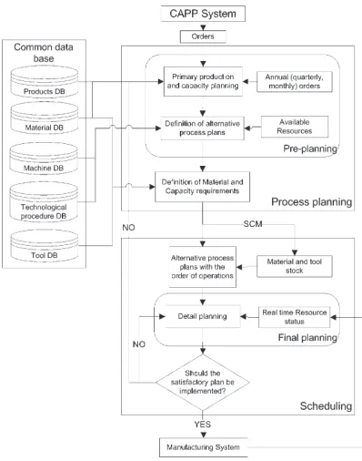
system, which represents the backbone of our dynamic planning system. Fig. 1 shows the overall procedure for the integration of
the
production planning and scheduling functions. It is basically divided into two modules – the first module or production planning module, where all alternative plans for each product are determined, and the second module or scheduling module with the genetic algorithms approach. In the first module, the static or pre-planning phase is performed, with the emphasis on specifying various plans according to available resources and specifyingproduction quantities and material needs. The
second module involves the final planning phase, where target functions and realistic conditions in the manufacturing environment are considered.
This means that the available resources are
matched with the required ones. If the current capacity does not meet the requirements, an extra plan should be included in the process. In practice,
this means that a product is being manufactured simultaneously on two machines.
First, from the CAPP system all orders are collected, followed by making a rough plan by means of gathering the information on the available capacity of regular orders that are always manufactured on a single machine. For other orders, alternative plans are prepared according
to other available resources. This is followed by
specifying material needs and capacity for all production quantities.
Fig. 1. Integratedmodel with production planning and scheduling function
When alternative plans, manufacturing
time, another aim is to achieve the most effective utilisation of machines, reduction of set-up times for the first operation and to minimise order delays.
Once a satisfactory schedule has been completed, it is considered as a working frame. If urgent orders arrive after the schedule has been completed, certain tasks are given higher priority. If an order has been cancelled or there is an equipment failure, a new schedule should be created. Due to the above-mentioned reasons it again functions as a frame. If there are no modifications, the optimum schedule should take place on the shop floor.
The following assumptions have been
specified for the solution of such a problem:
• Only one product can be produced on one machine at the same time;
• Each product can be machined independently from other products;
• Each product has one to three alternative plans (different CNC machines);
• The sequence of operations is predefined for
each product in the alternative plan.
3.1 Advantages and Disadvantages of the Proposed Method
The integration of production planning
and scheduling has led to the shift from manual scheduling to automated, computer-aided planning. Defining a detailed time when the manufacturing process of an order will start and when it will end, including delivery time, is the biggest advantage. Each operation on a product has a specified start time and end time. For example, it is specified when and how many products should be ready for galvanic coating. A planner is now able to check in any given moment which products are being produced on which machines and how many of them are on each operation. Such a planning method gives a planner a more supervisory role as they can follow via the information system what goes on on the shop floor and is informed whether an order is behind or ahead of schedule.
Manual methods include a lot of verbal communication with the shop floor, physical checks of machines on the progress of the work,
which is now no longer necessary. The automated
planning and scheduling system also allows control over finished products, material and tools. Planning requires consistency in the monitoring of products on each operation throughout the
manufacturing process. This information allows
an accurate prediction of how many products
can be finished in a short period of time. This is
important in the case of increased demand for
a product by a customer. The most important
thing for managing a dynamic manufacturing environment is a quick and efficient response to changes, such as machine failure, maintenance
work, and urgent orders. This means that if the
machine breaks down, then new borders are put
into the planning system. The products that have
already been put on the machine get the status “in progress” and they cannot be withdrawn, but the products with the “plan” status can be rescheduled.
This status is written in the ERP system. The same
procedure applies to urgent orders. A new plan can be made any time, the response time for a new plan is 15 minutes, on average. Information about the finished operations from the production
is an automatic update in the ERP system every 30
minutes.
Managing changes of materials and tools delivery dates by suppliers could be a drawback of production planning. If materials and tools are out of stock or they are not supplied on the planned date, the plan is unworkable and should be delayed by at least one day, which can trigger delays in the supply of end products.
4 USER INTERFACE BETWEEN ERP SYSTEM AND SCHEDULE OPTIMISATION
SOFTWARE
A manufacturing information system is the backbone of the planning and managing of production, which is why the existing information system within the planning model has been complemented rather than replaced. All data are
stored in the ERP information system. In order
to calculate the near optimum plan and schedule, data are exported and optimisation of the plan with
genetic algorithms is performed. The collected
data are then returned to the information system.
The whole system of data management is shown
Data are exported from the information system with the Oracle Discoverer 4.1 application.
The proposed algorithm is performed once a
day or at a request into a purpose built software
application (relational base MS Access, Visual Basic). Later, a transition to Oracle base and
C++ is planned. A genetic algorithm was used and proved very fast and with good conversion
results. This local base is the groundwork for
planning on the basis of the data from the basic
information system. The optimisation procedure
results in a detailed plan and schedule of products manufacturing. It serves as input information and enables the planner to generate manufacturing
product tasks within the ERP system.
Fig. 2. Data flowchart
The Oracle Discoverer application allows
access to the data base, located in the information
system. Each ERP session has a table with data
that are also visible in the session itself. Necessary information is specified in the Oracle Discoverer
application. The application also allows data
filtering, additional equations-based restrictions,
similar data pooling etc. The selected data
are exported into the local relational base that functions as the basis for planning and scheduling.
The relational data base is created in MS Access
which serves as the basis for the plan. Each field is
written in the same way as in the table in the ERP (Baan) system. The same applies to tables names.
A purpose application has been created for
the optimisation process. On the basis of the ERP
information system it schedules the activities on the shop floor in real time. Genetic algorithms
have proved to be an efficient method for product scheduling.
5 GENETIC ALGORITHM-BASED APPROACH FOR PRODUCTION
SCHEDULING
Genetic algorithms (GA) are a method of evolutionary computation. Genetic algorithms are a random search technique, not requiring detailed knowledge about a problem that is being optimised.
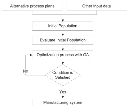
Fig. 3 shows the application of the genetic algorithm procedure. At the beginning, all alternative plans and other relevant information for the calculation of a satisfactory plan are gathered. Other data include delivery dates, stock information, materials and tools supply. In the next step, a population is randomly generated. It consists of a large number of different possible plans. On the basis of target functions and restrictions, each chromosome of
the initial population is evaluated. The evaluation
process is then carried out, with better and better solutions being sought on the basis of selection, reproduction, crossover and mutation until the
required condition is reached. The condition in
our case was a maximum number of generations.
Fig. 3. Course of the application of the genetic algorithm
Genetic algorithms represent solutions of
problems in structures, called chromosomes. The
and specific chromosomes in the population are individuals. A population at any given time
is called a generation. The goal of genetic
algorithms is to create new generations. Although the population can change from generation to generation, the size of the population and the
structure of chromosomes remain the same. They
operate with characters, representing parameters. Proper specification of parameters or chromosome syntax is an important step. It has an effect on subsequent work with genetic algorithms and on the share of workable solutions in the search area in terms of a large number of plans and
restrictions. The literature has so far presented the chromosome in a number of ways [25]. Below
are presented the chromosome, the evolutionary function with restrictions and genetic operators.
The chromosome has been adapted to the needs of
the production of turned parts.
5.1 Chromosome Representation
A job-based representation of a chromosome has been chosen to represent
the chromosome of the given problem. The
manufacturing type in the company is by orders. One product is represented by one gene in the
chromosome. The gene is represented by two
pieces of information, with the first one being the number of the alternative plan according to which the product will be manufactured while the other one specifies whether tools presetting
will take place (number 1) or not (number 0). The gene can be extended to other characteristics. The chromosome is shown in Fig. 4. The chromosome
is made up of a group of genes. In our case this is the schedule of all the products to be
manufactured. This means that the chromosome represents a permutation of tasks. Representation
of the chromosome by products belongs to direct approaches, where the solution is built in the chromosome. Genetic algorithms are used for the creation of the chromosomes whose objective is to find a better schedule. First, operations of the first product in the chromosome are scheduled
across machines. They are followed by the second
product’s operations and so on to the last one in the chromosome.
When the target function of the
chromosome is calculated, it has to be decoded
back to the solution of the problem, which means the schedule of products. During the encoding it is of the utmost importance to keep the subsequent solution of each chromosome decoded within
the possible space of a given problem. This feature is called feasibility. When the generated
chromosome cannot be decoded into a solution,
correcting techniques are applied. They change an illegal chromosome into a legal one. This feature
is called illegality.
Fig. 4. Chromosome
The relational database contains
information on products that is used for the
purpose of order scheduling. The list of genes or
the chromosome represents one possible schedule on the shop floor. Using GA, a satisfactory schedule, as close to the optimum as possible,
should be found. The GA principle is similar to
natural evolution. Only the strongest individuals survive, creating a new and more advanced population of descendants by means of gene mutations and their crossover.
5.2 Evaluation Functions
The shortest makespan and minimum
manufacturing costs were set as target functions and manufacturing restrictions and customers’ requirements were considered. Delivery time is the most important customer requirement. Other restrictions and criteria are described later on. Special emphasis is on the products where one of the operations is performed at an outsourcer.
Together with the making itself, the manufacturing
time also involves machine set-up and finishing
times. Total costs consist of manufacturing costs,
labour costs and depreciation costs. Mathematical model symbols:
N Number of orders or work orders,
A Number of items on the bill of material,
M Number of machines on the shop floor,
Pi Number of alternative plans for product i,
oilk k-operation for product’s i plan l,
Qo,i Ordered quantity of product i,
Qp,i Quantity of product’s i workpieces, overlapping with the next operation,
tpo,ilkj Time of operation’s oilk overlap on machine
j,
tt,ilkj Technological time for the production of one product i for operation oilk on machine
j,
tw,ilkj Processing time for operation oilk on machine j,
top,ilkj Time of the performance of operation oilk on machine j
tpz,ilkj Set-up and finishing times of machine j for operation oilk
tes,ilkj The earliest beginning of operation oilk on machine j
tef,ilkj The earliest end of operation oilk on machine j (df,ilkj)
tp,i Product’s i throughput time
tp,j Throughput time for all operations, performed on machine j, i.e. total time when a machine is engaged in the performance of all planned operations
ts,ilkj Set-up time of machine j for operation oilk
tmo,ilkj Time of interoperational hold-up for operation oilk on machine j
wi Product i priority
dd,i Scheduled delivery date of product i to the customer
tp,max Maximum time on machine among all machines
cssc,i Manufacturing costs for one piece of product i (all operations, materials, tools)
cd Labour costs
ca,j Depreciation cost for machine j
cs,ilkj Cost of machine j for operation oilk
cpz,ilkj Cost of operation’s oilk set-up and finishing time on machine j
cw,i Total cost for processing all operations for product i
cp,i Total costs for product i
C Total costs for all products
mnuj Non-utilisation of machine j
MU Maximum utilisation of all machines D Large positive integer
Zi Delivery delay of product i (in the number of days)
cwf Combined weighted function
λ Weight of delay
δ Costs of 1 day delay of the delivery date
αii j
i i j ´ ; ´ ; = 1 0
product appears before product on machine product DOES NOT appear
before product on machine
i
i´ j
βil= 1 i
0
; alternative plan for product IS selected ;; alternative plan for product IS NOT selectedi
γilk= 1
0 ; ;
operation is performed simultaneously operation iss performed sequentially
Target functions:
a) Minimum throughput time of all tasks and operations on a single machine:
Min tp,max=Max t t
{
p,1, p,2,...,tp M,}
, j=1,...,M,tp j top ilkj il
k G
l P
i
N i il
, =
(
, ⋅)
= = =∑
∑
∑
β 1 0 1 . (1)Time of the performance of operation:
top ilkj, =tpz ilkj, +tw ilkj, =tpz ilkj, +tt ilkj, ⋅Qo i,. Overlap time:
tpo ilkj, =tt ilkj, ⋅Qp i,.
b) Timely delivery with minimum delays:
Min Zmax=Max Z Z
{
1, ,...,2 ZN}
,i=1,...,N,
Z d d
d d
i
d i f ilG
f ilG d i
il il = > −
0 ; if
otherwise
, ,
, , ; ,
df ilG, il =tef ilG j, il .
(2)
c) Minimum total manufacturing costs for all products:
C Min cp i i N = =
∑
, 1 ,cp i cpz ilkj cs ilkj il c
j M k G l P w i il i , =
(
(
, + ,)
⋅)
+ , = = =∑
∑
∑
β 1 1 0 . (3) Processing costs:Machine costs:
cs ilkj, =top ilkj, ⋅ca j, . Set-up and finishing time costs:
cpz ilkj, =tpz ilkj, ⋅cd .
d) Combined weighted function:
cwf c c
c Z Z
p i z i i
N
z i i i
=
(
+)
= ⋅ ⋅ =∑
, , , , ( ^ ) . 1λ δ (4)
e) Maximum utilisation of all machines:
MU mnu mnu t t j j M j w ilkj i N j = = − = =
∑
∑
1 1 1 1 min , , max, =;j 1,..., .M
(5)
All restrictions have to be considered for an optimum manufacturing schedule of turned parts.
They are listed above. Below, they are presented
in a mathematical form.
Restrictions:
a) Only one product can be processed on each machine at the same time:
If d d then
t t D t
d i d i
p i l k j p ilkj ii j w i l k j
, , ´
, ´ ´ ´ , ( ´ ) , ´ ´ ´
<
− + ⋅ −1 α ≥ . (6)
b) Sequence of operations is predefined for each product in the alternative plan:
t t t t
i N l
es ilkj, w ilkj, pz il k, ( ) ´j es il k, ( ) ´j
,..., ; ,
+ + ≤
= =
+1 +1
1 0 ...., ; ,... ;
, ´ ,..., .
P k G
j j M
il = = 1 1 (7)
c) Only one alternative plan can be selected for one product.
Assumption:
w w
i N
il i l
il l Pi > = ∀ ∈
[ ]
+ =∑
( ) , 1 0 1 1β . (8)
d) Operation is performed simultaneously or sequentially.
Product's throughput times change because operation can be performed simultaneously or sequentially.
Throughput time for product i where operations are performed sequentially:
tp i tef ilG j tes il j top ilkj tmo ilkj
k G il il , = , − , =
(
, + ,)
=∑
11 . (9)
Throughput time for product i where operations are performed simultaneously:
t t t t t
t
p i pz ilkj po ilkj mo ilkj
k G
op ilG j
mo il il , , , , , , , =
(
+ +)
+ = −∑
1 1iilkj=tes il k, ( +1) ´j −tef ilkj, .
(10)
e) Throughput times for each operation and
product costs have to equal or exceed 0:
tp ilkj, ≥0 ; cp i, ≥0, (11)
i=1,..., ;N l=0,..., ;P ki =1,... ;G jil =1,..., .M (12)
Target functions equations are written from Eqs. (1) to (5). Taking account of all the objectives can be termed a multi-objective problem. The
most important objectives to achieve are minimum throughput time Eq. (1), timely delivery Eq. (2) and minimum total costs Eq. (3). Combined weighted function Eq. (4) is composed of total costs and delays. It is necessary to achieve the highest possible efficiency of machines Eq. (5), which reduces idle time on a machine.
Restrictions that appear in the algorithm are
written from Eqs. (6) to (10). Eq. (6) determines that a machine can produce only one product
at a time. The sequence of operations for two
different products on the same machine depends on the delivery date. It applies to all operations for all products. Eq. (7) determines the sequence of operations to be fixed for each product. It further increases the complexity of the problem. Only one alternative plan can be used for each product,
which is shown in Eq. (8). The first alternative
determine a product’s throughput time according
to the way of operations performance. The
algorithm also takes account of the fact that some operations take place consecutively and others simultaneously. Eq. (11) determines throughput time of each operation and all product costs should equal or exceed 0.
5.3 Genetic Operators
5.3.1 Selection
Tournament-type selection was used.
For this selection type, a certain number of chromosomes is selected, which then take part in
the tournament. Two individuals are matched and
the chromosome with the best value is selected. If the number of chromosomes to be matched increases in an algorithm, the pressure on the selection increases. Inferior chromosomes are not selected and thus do not take part in the creation of the next generation while at the same time good individuals also do not dominate the reproduction process.
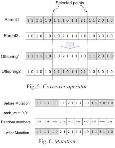
5.3.2 Crossover
Two-point crossover was chosen as the
crossover operator. Selected from the population
are two parents who form two offspring. Two
random points are selected in the chromosome, as
shown in Fig. 5. The material between both points is exchanged between the parents. This always creates feasible solutions. The crossover operator
is subjected to the probability that determines the use of the crossover chromosome.
5.3.3 Mutation
A mutation is about introducing new genetic material in the existing chromosome. It introduces variety in the population and broadens the search area. A mutation as well as crossover is subjected to some probability. For the existing
problem, the uniform mutation was selected. This
mutation is about each gene in a chromosome being attributed a random number, which is then matched with the probability of mutation. If the random number is smaller, the gene is
subjected to a mutation. This is shown in Fig. 6.
Genetic operators were selected on the basis of
a systematic comparison between the results of optimising and the necessary calculating time.
Fig. 5. Crossover operator
Fig. 6. Mutation
6 EXPERIMENTAL RESULTS
During the development of the genetic algorithm, several set-ups and approaches were
systematically tested. Tests showed that with
roughly 1000 evaluations it is possible to find a
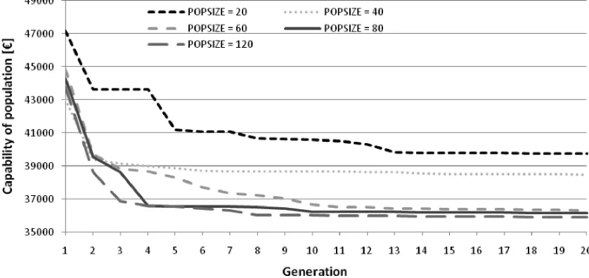
satisfactory solution for a plan. The size of the
population was limited to 60. A larger population extends the calculation time while there are no
significant savings with the population sizes of 80
and 120 (Fig. 7).
The optimum selection was determined
after comparing selections without the use of
crossover and mutation operators. The roulette
and tournament selections proved to be the best.
Two-point crossover with one-point
in the final version. The crossover probability is
set at 0.9 and the mutation probability at 0.01. For the purpose of determining the optimum solution for the production of a product or a product range, several alternative plans were
used for each product. These plans are entered
in the information system and their numbers of operations and designated machines for each
operation are already specified. Thirty products
were scheduled onto eighteen CNC machines
in the case study. There are thirty machines and ninety-five operations all together. There can be
up to four operations on a particular product and up to three alternative plans. Planned time in hours and machines for particular operations are
shown in Table 1. In the case of alternative plans
additional machines are specified in the same way as with products J2, J4 and J5. In parenthesis, the machine is marked with M and next to it is the number of the machine.
Fig. 7. Influence by size of population on convergence
Table 1. Processing time of all operations for a job with alternative plans
Jobs Operation 1 Processing timeOperation 2 Operation 3 Operation 4
Plan 1 Plan 2 Plan 3
J1 30.3 (M13) / / 0.8 (M19) 2.8 (M27)
J2 35.1 (M10) 33.6 (M8) 33.6 (M15) 1.21 (M19) 1.04 (M22) 17.42 (M26)
J3 92.1 (M13) / / 1.3 (M19) 11.1 (M27)
J4 10.8 (M10) 8.9 (M12) / 0.3 (M19) 0.3 (M27)
J5 9.6 (M10) 8.7 (M12) / 0.3 (M19) 0.4 (M27)
Table 2. Results from the initial plan
Total costs
[€] Throughput time [h] Makespan [h] Sum of delays [day]
Utilization of all machines
[%]
Combined weighted
function
[EUR]
Initial
For each target function an almost optimum solution was found with genetic algorithms.
Solutions are good enough � satisfactory for production scheduling. Better solutions do exist
but a minor difference does not make up for
additional calculation time. The objective is to find
the near optimum or satisfactory manufacturing plan out of the alternative plans in order to achieve good result of the fitness function.
The results of different target functions are summarized in Table 3. The size of the population
was set to sixty and the number of generations to fifty. Calculation time on a middle class personal
computer was 280 seconds for each target function from Table 3. The almost optimum solutions for
particular target functions are highlighted. Other values in the same line are given for a comparison between different target functions. Each target function achieves the best result in the column
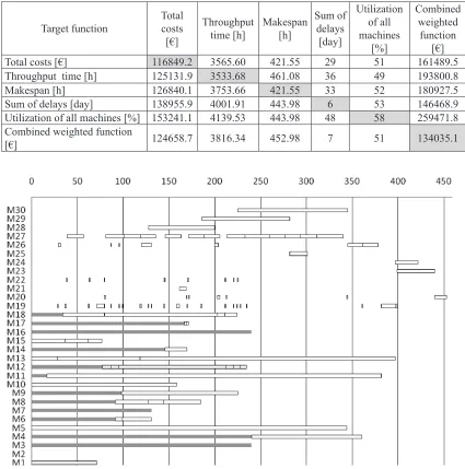
Table 3. Comparison between the values of target functions
Target function Total costs [€]
Throughput
time [h] Makespan [h]
Sum of delays
[day]
Utilization of all machines
[%]
Combined weighted
function [€]
Total costs [€] 116849.2 3565.60 421.55 29 51 161489.5
Throughput time [h] 125131.9 3533.68 461.08 36 49 193800.8
Makespan [h] 126840.1 3753.66 421.55 33 52 180927.5
Sum of delays [day] 138955.9 4001.91 443.98 6 53 146468.9
Utilization of all machines [%] 153241.1 4139.53 443.98 48 58 259471.8
Combined weighted function
[€] 124658.7 3816.34 452.98 7 51 134035.1
– it matches expectations. Special attention was paid to delivering products on due dates and to
control costs at the same time. We have set up a
Combined weighted function model that considers
both criteria: due date and costs. The comparison
between the first and the second target function reveals that the results are very similar. Due to
bigger makespan, the Throughput time function
yields more delays and higher additional costs. In that case products are not well scheduled on the machines.
According to the minimum delays criteria the fourth target function is the best choice. In this case, products extend the throughput time and increase total costs although combined costs are at
an acceptable level. The delays are only 6 days. The last of the target functions is a combined
weighted function. It represents a compromise
between total costs and delays. The value of this target function from Table 3 is not optimal, but itis a good solution acceptable to be used in practice.
Attention was also paid to the busiest machines on the shop floor and utilization of
the machines. The maximum utilization target function, where the result is 58%, the order of the
products on the machines causes the longest delay.
This is probably due to the order of the products
on the machines. All products produced together result in very good efficiency, but some products will be delayed because of this.
Other researchers report that 1200 calculations with the genetic algorithm represent a good enough solution that could be put into practice. In our case there were 3000 calculations.
Fig. 8 shows the Gantt chart for all
operations from the scheduling problem. On the vertical line are machines and time in hours is on the horizontal line. Each rectangle represents one operation. From the chart it can be seen that on machine 19 operations take a shorter time.
This is the deoiling machine and it can operate
with many parts concurrently. Machines M20 to
M22 are galvanizing machines. Those machines
operate also with big product batches. Makespan
for the presented schedule is 452.98 hours, which can be seen in Fig. 8. Some machines do
not operate at all. All alternative plans for each product were considered during the optimisation process and those machines were not chosen in any satisfactory scheduling plan. Machines
from M1 to M18 are CNC machines. For these
machines we also considered the working time at the beginning of the scheduling. If a machine is not available at the beginning the grey rectangle
in Fig. 8 shows finished time of the production.
And after that the product can be scheduled on
this machine. We believe that the major problem
in this example was scheduling on CNC machines because the operations are the longest. Machines from M19 to M30 represent the second operation,
third operation, etc. These operations mostly take
a short time and operate with big product batches.
The proposed genetic algorithm was tested on a similar problem from Gao et al. [23]. There
are six jobs and five different machines, each job
has several alternative plans. The results are in Table 4. Makespan is the result of the algorithm.
Probability pr, pc and pm are settings of probability for reproduction, crossover and mutation, respectively.
Computation time cannot be directly compared as it was not recognized as bottle-neck due to different programming environments.
When the target functions (makespan) the results are close together. The proposed GA results in
longer makespans, but it is good enough for
practical application. The results from all cases of the proposed GA are almost the same. The
increase of the population size in this simple problem does not yield significantly better results.
The closest makespan is achieved in the second case. With a population size ten times smaller, almost the same result is obtained. We believe that
the result in the second case is satisfactory for this simple problem.
After all these comparisons a specific solution for the production of turned parts’ has been created: combined weighted function offers the satisfactory solution. From the point of view of the sales department, minimum delays are top priority, while on the other hand, for the production department and management, minimum costs are
top priority. This target function allows both.
7 CONCLUSION
This article has shown how to apply a
convincing, which could result in a dead end. For this reason, it is vital to check combinations of different target functions as in the case of
combined weighted function. The proposed
criterion for the production of turned parts includes total costs and delays. For the lowest common costs, additional delays will have to be accepted.
Table 4. Comparison of the results
Gaos’
approach Proposed GA
Code C++ VB
Computer Core ™2 2Ghz Duo CPU
1.66 Ghz Core™2 CPU 1st
case case2rd case3rd
Pop size 200 200 20 60
Max gens 50 50 50 50
Iterations 20 20 20 20
pr 0.1 0.1 0.1 0.2
pc 0.8 0.8 0.8 0.9
pm 0.1 0.1 0.1 0.01
Makespan 92 96 95 96
Finally, it was possible to compare the results from the selected target function and the
initial plan, shown in Table 2. It was applied on
the machine according to when the orders reached our company and for each job first an alternative
plan was chosen. The costs of the combined
weighted function drop by 69.1%. 15.6% amount to the total cost, while the rest is owing to the
machines being chosen correctly. The makespan moves from 1257.58 to 452.98 hours. The amount
of saving is the result of our strong emphasis on delays. For this reason a special weight has been developed.
In addition to planning and scheduling of manufacturing activities, the presented model also allows optimisation of manufacturing plans and machines. In this case the solution area is much larger due to the fact that all available machines are varied within each operation of the plan. It is possible to also take account of the machines that are not yet present in the existing plans or exist only in investment plans.
8 ACKNOWLEDEGMENT
The research is supported by the Ministry of Higher Education, Science and Technology under the project P-MR-08/88. Operation part
financed by the European Union, European Social Fund.
9 REFERENCES
[1] Errington, J. (1997). Advanced Planning and Scheduling (APS): a powerful emerging technology. Next Generation I.T. in
Manufacturing, no. 315, p. 3/1-3/6.
[2] Tasič, T., Buchmeister, B., Ačko, B. (2007). The development of advanced
methods for scheduling production process. Strojniški vestnik – Journal of Mechanical
Engineering, vol. 53, no. 12, p. 844-857.
[3] Alting, L., Zhang, H-C. (1989). Computer
aided process planning: the state-of-the-art survey. International Journal of Production
Research, vol. 27, no. 4, p. 553-585.
[4] Huang, S.H., Zhang, H-C., Smith, M.L. (1995). A progressive approach for the integration of process planning and scheduling. IIE Transactions, vol. 27, no. 4, p. 456-464.
[5] Tan, W., Khoshnevis, B. (2000). Integration
of process planning and scheduling – a review. Journal of Intelligent Manufacturing, vol. 11, no. 1, p. 51-63.
[6] Kumar, M., Rajotia, S. (2003). Integration
of scheduling with computer aided process planning. Journal of Materials Processing
Technology, vol. 138, no. 1-3, p. 297-300.
[7] Larsen, N.E. (1993). Methods for integration of process planning and production planning. International Journal of Computer
Integrated Manufacturing, vol. 6, no. 1-2, p.
152-162.
[8] Wang, L., Shen, W. (2003). DPP: An
agent-based approach for distributed process planning. Journal of Intelligent
Manufacturing, vol. 14, no. 5, p. 429-439.
[9] Zhang, H-C. (1993). IPPM - A prototype to integrate process planning and job shop scheduling functions. CIRP Annals –
Manufacturing Technology, vol. 42, no. 1, p.
[10] Gao, L., Shao, X., Li, X., Zhang C. (2009). Integration of process planning and scheduling – A modified genetic algorithm-based approach. Computers & Operation
Research, vol. 36, no. 6, p. 2082-2096.
[11] Usher, J.M., Fernandes, K.J. (1996). Dynamic process planning – the static phase. Journal of Materials Processing
Technology, vol. 61, no. 1, p. 53-58.
[12] Kumar, M., Rajotia, S. (2006). Integration
of process planning and scheduling in a job shop environment. International Journal of
Advanced Manufacturing Technology, vol.
28, no. 1-2, p. 109-116.
[13] Jain, A., Jain, P.K., Singh, I.P. (2006). An Integrated scheme for process planning and scheduling in FMS. The International
Journal of Advanced Manufacturing
Technology, vol. 30, no. 11-12, p. 1111-1118.
[14] Haddadzade, M., Razfar, M.R., Farahnakian,
M. (2009). Integrating process planning and scheduling for prismatic part regards to due date. World Academy of Science,
Engineering and Technology, vol. 51, p.
64-67.
[15] Starbek, M., Potočnik, P., Grum, J., Berlec, T. (2008). Predicting Order Lead Times. Strojniški vestnik – Journal of Mechanical
Engineering, vol. 54, no. 5, p. 308-321.
[16] Kopač, J., Soković, M., Rosu, M., Doicin,
C. (2005). Quality and cost in production management process. Strojniški vestnik –
Journal of Mechanical Engineering, vol. 54,
no. 3, p. 207-218.
[17] Balič, J., Ficko, M., Brezočnik, M. (2005). A
model for forming a flexible manufacturing system using genetic algorithms. Strojniški vestnik – Journal of Mechanical
Engineering, vol. 51, no. 1, p. 28-40.
[18] Yan, H-S., Zhang, X-D. (2007). A case study on integrated production planning and scheduling in a three-stage manufacturing
system. IEEE Transactions on automation
science and engineering, vol. 4, no. 1, p.
86-92.
[19] Park, B.J., Choi, H.R. (2006). A genetic
algorithm for integration of process planning and scheduling in a job shop. AI2006:
Advances in Artificial Intelligence, p.
647-657.
[20] Kimms, A. (1999). A genetic algorithm for multi-level, multi-machine lot sizing and scheduling. Computers & Operations
Research, vol. 26, no. 8, p. 829-848.
[21] Zhang, X.-D., Yan, H.-S. (2005). Integrated optimization of production planning and scheduling for a kind of a job. The
International Journal of Advanced
Manufacturing Technology, vol. 26, no. 7-8,
p. 876-886.
[22] Lee, H., Kim, S.-S. (2001). Integration of process planning and scheduling using simulation based genetic algorithms. The International Journal of Advanced
Manufacturing Technology, vol. 18, no. 8, p.
586-590.
[23] Li, X., Gao, L., Shao, X., Zhang, C., Wang,
C. (2010). Mathematical modeling and evolutionary algorithm-based approach for integrated process planning and scheduling.
Computers and Operations Research, vol.
37, no. 4, p. 656-667.
[24] Lestan, Z., Brezočnik, M., Buchmeister, B., Brezočnik, S., Balič, J. (2009). Solving the
job-shop scheduling problem with simple genetic algorithm. International Journal of
Simulation Modelling, vol. 8, no. 4, p.
197-205.
[25] Cheng, R., Gen, M., Tsujimura, Y. (1996).
A tutorial survey of job-shop scheduling problems using genetic algorithms – I: representation. Computers and Industrial