in the population sciences published by the Max Planck Institute for Demographic Research Konrad-Zuse Str. 1, D-18057 Rostock · GERMANY www.demographic-research.org
DEMOGRAPHIC RESEARCH
VOLUME 22, ARTICLE 17, PAGES 505-538
PUBLISHED 26 MARCH 2010
http://www.demographic-research.org/Volumes/Vol22/17/ DOI: 10.4054/DemRes.2010.22.17
Research Article
The compression of deaths above the mode
A. Roger Thatcher
Siu Lan K. Cheung
Shiro Horiuchi
Jean-Marie Robine
© 2010 A. Roger Thatcher et al.
This open-access work is published under the terms of the Creative Commons Attribution NonCommercial License 2.0 Germany, which permits use, reproduction & distribution in any medium for non-commercial purposes, provided the original author(s) and source are given credit.
1 Background 506
2 Methodology 508
2.1 Definition and estimation of e(M) and SD(M+) 508
2.2 Choice of model 508
2.3 Estimating b and predicting M, e(M), and SD(M+) 512 3 Illustrations for England and Wales 514 4 Results for six countries 518 4.1 Trends in the parameter b 518
4.2 Mode and SD(M+) 519
4.3 Accuracy of the predictions of SD(M+) 523
5 Discussion 527
6 Acknowledgments 528
References 529
Appendix 532
A1 M, e(M), and SD(M+) for a continuous distribution 532 A2 Approximations when the distribution is discrete 532 A3 Different versions and derivations of the logistic model 533
A4 Proof of equation (4) 535
A5 Proof that in the simple logistic model, e(M) and SD(M+) are determined solely by b, independently of M
536
A6 Proof of equation (10) 537
The compression of deaths above the mode
A. Roger Thatcher1 Siu Lan K. Cheung2 Shiro Horiuchi3 Jean-Marie Robine4
Abstract
Kannisto (2001) has shown that as the frequency distribution of ages at death has shifted to the right, the age distribution of deaths above the modal age has become more compressed. In order to further investigate this old-age mortality compression, we adopt the simple logistic model with two parameters, which is known to fit data on old-age mortality well (Thatcher 1999). Based on the model, we show that three key measures of old-age mortality (the modal age of adult deaths, the life expectancy at the modal age, and the standard deviation of ages at death above the mode) can be estimated fairly accurately from death rates at only two suitably chosen high ages (70 and 90 in this study). The distribution of deaths above the modal age becomes compressed when the logits of death rates fall more at the lower age than at the higher age. Our analysis of mortality time series in six countries, using the logistic model, endorsed Kannisto’s conclusion. Some possible reasons for the compression are discussed.
1 Former Director of the Office of Population Censuses and Surveys, London. Roger Thatcher passed away in
February 2010, after this paper was accepted but before it could be published.
2 Faculty of Social Sciences, The University of Hong Kong.
3 CUNY School of Public Health, CUNY Institute for Demographic Research, The City University of New
York.
1. Background
The substantial decline of overall mortality since the nineteenth century made it possible for a larger proportion of people to survive to old ages, thereby concentrating deaths into a relatively narrow range of old age. This has made the survival curve (the table l(x) function) more rectangular and the age distribution of deaths (the life-table d(x) function) more compressed (Comfort 1956; Fries 1980; Wilmoth and Horiuchi 1999).
The considerable decline of death rates in childhood and young adult ages during the first half of the twentieth century was the major driving force of the mortality compression. Then, significant declines in old-age mortality started in economically developed countries during the second half of the twentieth century (Kannisto et al. 1984). In this period, the compression of the overall death distribution was slow, and even almost stagnant in some populations (Wilmoth and Horiuchi 1999; Yashin et al. 2001). Thus, changes in the distribution of adult deaths during the last few decades is shown to be approximated well by models in which the distribution is assumed to shift to the right without changing its shape (Bongaarts 2005; Canudas-Romo 2010, forthcoming).
However, in the context of the longevity extension, it has become increasingly important to distinguish old-age mortality compression from overall mortality compression, and to analyze changes in the shape of age distribution of deaths at very old ages separately from changes in the age distribution of deaths over the entire lifespan (or over a broad range of adult ages). Based on the model of death distribution by Lexis (1878), Kannisto (2000, 2001) focused on the modal age of adult deaths as an important central tendency measure of longevity, and examined the dispersion of deaths above the mode. He presented extensive evidence to show that the distribution of deaths at old ages was not simply sliding to the right. Instead, the right hand downward slope was being flattened vertically, so that the distribution became more compressed, as if (in his words) it was meeting an invisible wall. He contended that the ascending trajectory of mortality at high ages formed such a barrier but only in a relative sense, offering increasing resistance to further progress without setting any definite limit to it.
with focus on M has been elaborated further in recent studies by Cheung and her collaborators (Cheung et al. 2005, 2008, 2009; Cheung and Robine 2007; Robine et al. 2006) and Canudas-Romo (2010, forthcoming).
The mortality compression can be analyzed with respect to the age pattern of mortality (life-table m(x) or q(x) function) as well, because the q(x), d(x), and l(x) functions uniquely determine each other. In general, a faster mortality reduction at younger ages leads to a steeper age-associated increase in mortality, thereby concentrating deaths in older ages. Previous research on age patterns of adult mortality by Strehler and Mildvan (1960) and Gavrilov and Gavrilova (1991) are closely related to mortality compression. Using the international data, Strehler and Mildvan have shown that two parameters of the Gompertz model are negatively correlated, indicating the following tendency: as the level of adult mortality declines, the mortality curve rises more steeply upward. Gavrilov and Gavrilova use the Makeham model to show that the Strehler-Mildvan correlation is largely due to the substantial reduction of background mortality (premature mortality unrelated to senescence). However, even after the effect of background mortality has been removed, the two parameters of the Gompertz term of the Makeham model remain negatively associated, suggesting that the reduction of senescence-related mortality may produce some compression in the senescent death distribution.
The study by Strehler and Mildvan and that by Gavrilov and Gavrilova are based on the Gompertz model and Makeham model, respectively, and the data analyzed in those studies are mainly for periods before the onset of considerable decline in old-age mortality. However, an extensive analysis of old-age mortality data (Kannisto-Thatcher database) has revealed that the age-related mortality increase tends to slow down at very old ages, which cannot be captured by the Gompertz or Makeham model, and age patterns of old-age mortality are well represented by logistic models (Thatcher 1999; Thatcher et al. 1998).
2. Methodology
2.1 Definition and estimation of e(M) and SD(M+)
e(M) is defined as the expectation of life of those who have just reached the modal age of adult deaths. The upward standard deviation from the mode, SD(M+), is the root-mean-square of the lengths of life lived beyond the modal age. Note that e(M) can be considered a dispersion measure, because it is the upward mean deviation from the mode. If the age at death in the life table is considered a continuous random variable, then the mode M is the age with the highest density of adult deaths, while e(M) and SD(M+) are given by integrals of deviation and squared deviation, respectively, from the mode as shown in the Appendix, section 1.
Alternatively, if we are working from a complete life table which shows the number of persons out of 100,000 who die at age x, then there are various ways to estimate the mode M of a continuous age distribution. By shifting the origin to the mode, e(M) and SD(M+) can then be calculated from first principles by the method of moments. However, there are also short cuts, described in the Appendix, section 2.
2.2 Choice of model
With only one exception (males in England and Wales for 1900-04), all the modes in the data analyzed in this paper are above the age of 70. These modal ages are therefore determined by the distribution of the relative frequencies of deaths at each age over 70. Death rates below age 70 will determine the numbers of survivors who reach age 70, but they will not affect the relative frequencies for the ages at death above age 70. At least in a standard life table, these relative frequencies above age 70 are determined solely by the death rates at ages 70 and over. From the life table entries we can estimate not only M but also e(M) and SD(M+), so all three are determined by the death rates at ages 70 and over. In these circumstances, what are the conditions in which compression will occur?
this normal-distribution model fits the data on deaths above the mode very well, except perhaps at extreme ages in some populations (Cheung and Robine 2007).
In this paper, we combine Kannisto’s approach, which is based on the Lexis model, with the logistic model, which is known to fit empirical age patterns of old-age mortality well. We adopt a special case of the logistic model of mortality, which also has a long history and literature (see Thatcher 1999). This special case has only two parameters as does the Lexis model, and it is usually written in the form
μ(x) = a ebx / (1 + a ebx ) (1)
Here μx is the force of mortality at age x, while a and b are parameters which are constant in any given period (or in any cohort, if the model is applied to cohort mortality data).
Theoretical derivations of the logistic model are given in the Appendix, section 3. The simple logistic model has only two parameters, whereas the general logistic model has four. One of these four (Makeham’s constant) becomes significant at some stage below age 70, while another allows for alternative limits of mortality at extremely high ages, such as supercentenarians. For the present paper, however, we are not concerned with ages below 70 or with the most extreme high ages. Within the range to which we shall confine ourselves, the simple 2-parameter version seems to be adequate.
The model (1) can be written in a simplified form, if we make use of the mathematical function known as the logit function, which is only the difference between two logarithms. The logit function is defined by
logit (z) = ln(z/(1-z)) = ln z - ln (1-z) (2)
With this notation it is easily seen that (1) can be written as
logit (μ(x) ) = a* + bx (3)
where a* = ln a. If we calculate y = logit (μx) then the points (x, y) will lie on a straight line represented by equation (3). We shall call this the “logit line”.
It is shown in the Appendix, section 4, that if μx follows (1) then the modal age of death will occur at the age M which satisfies
aebM = b, (4)
which is equivalent to equation (20) in Robine et al. (2006) and equation (11) in Canudas-Romo (2008). It then follows that (1) can be written as
μ(M+y) = beby / (1 + beby ), for any y≥ 0 . (5)
The significance of this is that if we measure ages from the mode, then the whole shape of the distribution of both death rates and of ages at death depends only on the single parameter b, which summarises the age distribution of deaths above the modal age.
When b is known, equation (5) makes it possible to construct a theoretical life table with its origin at the mode. This life table will give the death rate at age y=x−M for y≥0, and this death rate will depend only on b and y. Thus the death rate at age y above the mode can be calculated without actually knowing the value of the mode. Since e(M) and SD(M+) can be calculated from the death rates above the mode, they too can be calculated from b, without knowing the mode. This is shown in a more formal manner in section 5 of the Appendix.
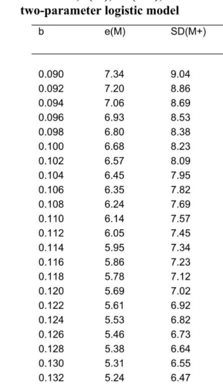
The numerical relationship is shown in Table 1. As expected, higher b values are associated with smaller e(M) and SD(M+) values, i.e., greater extents of compression.
If we know b, then we can simply read off the values of e(M) and SD(M+). Since 1900, with only one exception, all the estimated value of parameter b has been between 0.09 and 0.15, and the ratio of SD(M+) to e(M) has fallen in a very narrow band, between 1.231 and 1.235. (This parallels a fixed ratio of 1.253 in the Lexis model). In view of this proportionality, results for e(M) will always imply results for SD(M+), and vice versa.
A further important feature of the model is that while b determines the compression, as measured by e(M) and SD(M+), the two values a and b in conjunction enable us to calculate the mode M. From equation (4) it follows that
M = ln(b/a)/b = (ln b)/b – (ln a)/b . (6)
Table 1: Value of b, e(M), SD(M+), and ratio SD(M+)/e(M) derived from the two-parameter logistic model
b e(M) SD(M+) Ratio
SD(M+)/e(M)
0.090 7.34 9.04 1.2307 0.092 7.20 8.86 1.2309 0.094 7.06 8.69 1.2310 0.096 6.93 8.53 1.2312 0.098 6.80 8.38 1.2314 0.100 6.68 8.23 1.2315 0.102 6.57 8.09 1.2317 0.104 6.45 7.95 1.2318 0.106 6.35 7.82 1.2320 0.108 6.24 7.69 1.2322 0.110 6.14 7.57 1.2323 0.112 6.05 7.45 1.2325 0.114 5.95 7.34 1.2326 0.116 5.86 7.23 1.2328 0.118 5.78 7.12 1.2330 0.120 5.69 7.02 1.2331 0.122 5.61 6.92 1.2333 0.124 5.53 6.82 1.2334 0.126 5.46 6.73 1.2336 0.128 5.38 6.64 1.2338 0.130 5.31 6.55 1.2339 0.132 5.24 6.47 1.2341 0.134 5.18 6.39 1.2342 0.136 5.11 6.31 1.2344 0.138 5.05 6.23 1.2345 0.140 4.99 6.16 1.2347 0.142 4.93 6.08 1.2349 0.144 4.87 6.01 1.2350 0.146 4.81 5.94 1.2352 0.148 4.76 5.88 1.2353 0.150 4.70 5.81 1.2355
Appendix, section 7, the logistic equation of mortality can be derived from at least two sets of completely different assumptions: the frailty model of selective survival and the Le Bras model of stochastic ageing processes (Le Bras 1976). The Lexis model uses the normal distribution, which is approximated by the sum of a large number of independent and identically distributed random variables. The fact that these totally different assumptions produce almost the same results over a wide range of ages above the mode is therefore surprising, but also reassuring.
2.3 Estimating b and predicting M, e(M), and SD(M+)
In order to apply the simple logistic model, we need to be able to estimate the parameter b. Since b is the slope of the straight line (3), it is sufficient to know the value of µx at any two ages, say x1 and x2 , where x2 > x1. The slope of the line between these ages is then given by
b = [logit µ(x2) - logit µ(x1)] / (x2 - x1) (7)
However, since the central death rate m(x) at age x satisfies the approximation
m(x) ≈ µ(x + ½) (8)
we can use
b ≈ [logit m(x2 ) - logit m(x1) ] / (x2 - x1 ) (9)
to calculate b readily from life tables.
small number of deaths may notably increase the standard error of logit m(x2), and in turn, that of b.
In consideration of these issues, we chose age 70 and age 90 for x1 and x2, respectively. Age 70 seems appropriate because in the 80 life tables from the Human Mortality Database that we analyzed, the estimated M was above age 70 in all cases except males in England and Wales, 1900-1904, for which M was 69.85. As described later, we compared our results among three sets, ages 70-90, 70-80, and 80-90, and found parameter trends were less erratic for ages 70-90 than for ages 70-80 and 80-90.
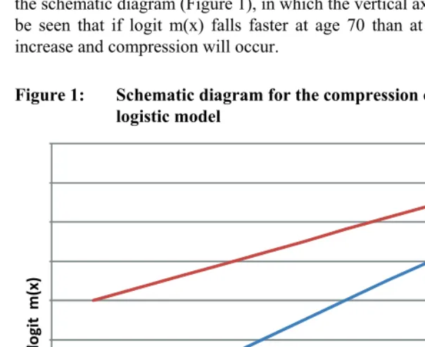
By comparing the estimates of b at two different dates, we can see whether b is increasing, and hence whether compression is occurring. The situation is illustrated in the schematic diagram (Figure 1), in which the vertical axis is taken as logit m(x). It can be seen that if logit m(x) falls faster at age 70 than at age 90, then the slope b will increase and compression will occur.
Figure 1: Schematic diagram for the compression of mortality in the simple logistic model
0 1 2 3 4 5 6 7 8 9
0 1 2 3 4 5 6 7 8 9 10 11 12
Mortality
X1
it
m(x)
Age X2
log
compression will occur if the death rates at ages 70 and over follow the simple logistic model, and change in such a way that logit m(x) falls faster at age 70 than at age 90.
Once the value of b has been obtained by applying equation (9) to death rates at ages 70 and 90, the modal age of adult deaths M can be predicted by
M = (ln b)/b – [logit m(x1)]/b + x1 + ½ (10)
where x1=70 in this study. Equation (10) is an approximated version of equation (6), as shown in section 6 of the Appendix. e(M) and SD(M+) can be obtained by numerical integration based on equations (A.13) and (A.14) in section 5 of the Appendix, or simply by interpolation of values in Table 1.
3. Illustrations for England and Wales
The illustrations which follow use data for England and Wales, obtained from the English Life Tables and Interim Life Tables.
Figures 2 and 3 show logit m(x) for males and females in England and Wales for 1906, 1971 and 2004. It can readily be seen that the observed points look fairly straight. These are the logit m(x) curves. It must be remembered that we are not formally fitting straight lines. We are only seeking confirmation that the observed points of logit m(x) are close enough to straight lines to justify the choice of the logistic equation as a simple working model. As can be seen at a glance, the lines do not all have quite the same slopes. The model therefore indicates that there were changes over time in the parameter b and hence in e(M) and SD(M+).
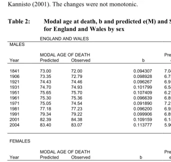
Figures 4 and 5 show how the modal ages of death have varied, using both observed values (full lines) and the predicted modes given by the simple logistic model (dashed lines). All the data which are plotted in these figures are given in Table 2, which also shows, for interest, the values for e(M) and SD(M+) predicted by the model. There are footnotes giving the sources and methods.
The predictions in Figures 4 and 5 were all made independently of each other, using only the observed death rates (and hence their logits) at ages 70 and 90. The predictions are reasonably close to the observed values.
Figure 2: Logit m(x) for males in England and Wales: 1906, 1971 and 2004
5 6 7 8 9 10
70 72 74 76 78 80 82 84 86 88 90 92 94
10
+
lo
gi
t
m(
x)
Age
1906 1971 2004
Figure 3: Logit m(x) for females in England and Wales: 1906, 1971 and 2004
5 6 7 8 9 10
70 72 74 76 78 80 82 84 86 88 90 92 94
10
+
lo
git
m(
x)
Age
Figure 4: Modal age of death for males in England and Wales, 1841-2004
70 72 74 76 78 80 82 84 86 88
1820 1840 1860 1880 1900 1920 1940 1960 1980 2000 2020
Ag
e
Year
Predicted
Observed
Figure 5: Modal age of death for females in England and Wales, 1841-2004
70 72 74 76 78 80 82 84 86 88
1820 1840 1860 1880 1900 1920 1940 1960 1980 2000 2020
Ag
e
Year
Predicted
The data are given in Table 2, which gives a conspectus of the changes in England and Wales over the whole period from 1841 to 2004, as derived from the national life tables. The mode M rose for both males and females. For males, e(M) and SD(M+) both rose and fell. For females, we see only falls and this is the progression observed by Kannisto (2001). The changes were not monotonic.
Table 2: Modal age at death, b and predicted e(M) and SD(M+) for England and Wales by sex
ENGLAND AND WALES
MALES
MODAL AGE OF DEATH Predicted Predicted
Year Predicted Observed b e(M) SD(M+)
1841 73.00 72.00 0.094307 7.04 8.68
1906 73.35 72.79 0.098928 6.75 8.32
1921 74.43 74.46 0.096267 6.91 8.52
1931 74.70 74.93 0.101799 6.58 8.11
1951 75.65 75.70 0.107409 6.27 7.73
1961 75.30 75.36 0.096639 6.89 8.50
1971 75.05 74.54 0.091890 7.21 8.89
1981 77.18 77.23 0.096200 6.92 8.53
1991 79.34 79.22 0.099906 6.89 8.50
2001 82.39 84.38 0.109159 6.18 7.62
2004 83.40 83.07 0.113777 5.96 7.35
FEMALES
MODAL AGE OF DEATH Predicted Predicted
Year Predicted Observed b e(M) SD(M+)
1841 74.31 73.67 0.095701 6.95 8.57
1906 75.14 74.00 0.096494 6.90 8.51
1921 77.46 77.15 0.100735 6.64 8.19
1931 78.05 77.86 0.107003 6.29 7.76
1951 80.28 80.25 0.116308 5.85 7.21
1961 81.45 81.42 0.116333 5.85 7.21
1971 82.50 82.42 0.113851 5.96 7.35
1981 83.62 84.33 0.115700 5.88 7.25
1991 84.75 86.17 0.112585 6.02 7.42
2001 86.36 86.30 0.120560 5.67 6.99
2004 86.93 87.76 0.124741 5.50 6.78
Sources: English Life Tables no 1, 1841; no 7, 1901-10; no 9, 1920-22; no 10, 1930-32; no 11, 1950-52; no 12, 1960-62; no 13, 1970-72; no 14, 1980-82; no 15, 1990-92. Interim Life Tables for England and Wales 2000-2002; 2003-5. These life tables were prepared successively by the Registrar General, the Government Actuary and now the Office for National Statistics.
4. Results for six countries
4.1 Trends in the parameter b
A further study on age patterns of mortality at high ages has been conducted using international mortality data in the HMD (Human Mortality Database 2007), not only for England and Wales but also for France, Japan, Italy, Sweden and Switzerland. Curves of logit m(x) between ages 70 and 90 have been drawn for each of these countries for every single year for which data are given in the HMD (Figures of these many lines are available on line at www.demographic-research.org/Volumes/Vol22/17/default.htm).
Visual inspection of those curves suggested that patterns and trends for those 12 (six countries times two sexes) sets of HMD life tables were similar to those in Figures 2 and 3 for English life tables: the curves were nearly or fairly straight (with some exceptions in early years and war/epidemic periods) but their slope appears to be increasingly steeper over decades.
We then examined this visual impression by estimating the parameter b from the slope of the logit line between ages 70 and 90. These ages were chosen with one below the mode and one above it, and with a span of 20 years in order to make the standard errors of the estimate of b small. If the data on deaths followed the simple logistic model exactly, any pair of ages in the range 70 and over would give the same estimate of b, but it is natural to wonder whether this holds in practice.
Accordingly, the slopes of the 80 logit lines described above were found from the pairs of ages 70-80, 80-90 and 70-90. Comparison showed that the differences among those slopes were mostly negligible. Any larger differences could only be due to the occasional “wobbles” in the logit lines. It was noticeable, however, that trends of the estimates based on 70-80 and 80-90 were more erratic, suggesting that they have more “noise” than the estimates based on 70-90.
In all cases, the b at the latest date was higher than the b at the earliest date, so the predicted standard deviation SD(M+) was lower at the later date. Thus over the period as a whole there had been compression above the mode in all six countries, for both males and females.
4.2 Mode and SD(M+)
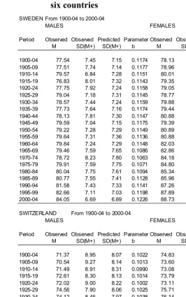
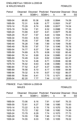
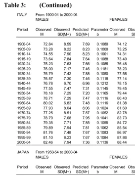
Time series giving the data for the six countries are assembled in Table 3. This shows for each country the observed value of the mode M, the observed value of the standard deviation above the mode SD(M+), the value of the parameter b found from the logit functions of the death rates at ages 70 and 90, and the prediction of SD(M+) given by b. Trends in the observed and predicted SD(M+) are also displayed in Figure 6. The table and figure enable us to see the differences between countries and to examine whether rises in the mode have always been accompanied by falls in the standard deviation. Comparisons between the observed and predicted values of SD(M+) also show whether the data support the theoretical deduction from the simple logistic model, that the standard deviation is related to the death rates at the high ages such as 70 and 90, so that it is the factors which affect these death rates differently which may be regarded as the ultimate causes of compression or decompression.
Table 3 gives the series for 5-year periods from 1900-1904 to 2000-2004 for Sweden, Switzerland, Italy, England and Wales and France, and from 1950-1954 to 2000-2004 for Japan. The methods by which the table was constructed are given in the Appendix, section 3.
The average changes can be summarised briefly as follows: for males in the five countries excluding Japan, the observed mode rose from 72.9 to 77.2 in the first fifty years, and from 77.2 to 83.5 in the second fifty years. The observed standard deviation SD(M+) fell from 8.7 to 7.7 in the first fifty years, and from 7.7 to 7.3 in the second. Thus, the rise in the mode sped up, but the fall in the standard deviation slowed down.
For females in these same countries, the average mode rose from 75.5 to 80.1 in the first 50 years, and from 80.1 to 88.5 in the second. The observed standard deviation fell from 7.9 to 7.3 in the first fifty years, and from 7.3 to 6.1 in the second. Again, the rise in the mode sped up, but for females the fall in the observed standard deviation accelerated.
Table 3: Modal age of death and the standard deviations above the mode for six countries
SWEDEN From 1900-04 to 2000-04
MALES FEMALES
Period Observed Observed Predicted Parameter Observed Observed Predicted Parameter M SD(M+) SD(M+) b M SD(M+) SD(M+) b
1900-04 77.54 7.45 7.15 0.1174 78.13 7.74 7.43 0.1125 1905-09 77.51 7.74 7.14 0.1177 78.96 7.56 7.24 0.1159 1910-14 79.57 6.84 7.28 0.1151 80.01 7.03 7.42 0.1126 1915-19 76.83 8.01 7.32 0.1143 79.35 7.34 7.48 0.1115 1920-24 77.75 7.92 7.24 0.1158 79.05 7.61 7.19 0.1168 1925-29 79.04 7.18 7.31 0.1145 78.77 7.65 7.27 0.1153 1930-34 78.57 7.44 7.24 0.1159 79.88 7.13 7.36 0.1137 1935-39 77.73 7.64 7.16 0.1174 79.44 7.09 7.17 0.1171 1940-44 78.13 7.81 7.30 0.1147 80.88 6.80 7.29 0.1149 1945-49 79.59 7.04 7.15 0.1175 79.39 7.49 6.93 0.1219 1950-54 79.22 7.28 7.29 0.1149 80.89 6.84 7.18 0.1169 1955-59 79.64 7.31 7.36 0.1136 80.88 7.24 7.05 0.1194 1960-64 79.84 7.24 7.29 0.1148 82.03 6.82 6.87 0.1231 1965-69 79.46 7.59 7.65 0.1086 82.86 6.76 6.74 0.1258 1970-74 78.72 8.23 7.80 0.1063 84.18 6.77 6.81 0.1244 1975-79 79.91 7.59 7.75 0.1071 84.80 6.68 6.72 0.1264 1980-84 80.04 7.75 7.61 0.1094 85.34 6.71 6.70 0.1266 1985-89 80.77 7.55 7.41 0.1128 85.96 6.55 6.59 0.1291 1990-94 81.58 7.43 7.33 0.1141 87.26 6.10 6.46 0.1321 1995-99 82.66 7.11 7.03 0.1198 87.89 6.02 6.42 0.1332 2000-04 84.05 6.69 6.89 0.1226 88.73 5.67 6.41 0.1334
SWITZERLAND From 1900-04 to 2000-04
MALES FEMALES
Period Observed Observed Predicted Parameter Observed Observed Predicted Parameter M SD(M+) SD(M+) b M SD(M+) SD(M+) b
Table 3: (Continued) ENGLAND From 1900-04 to 2000-04
& WALES MALES FEMALES
Period Observed Observed Predicted Parameter Observed Observed Predicted Parameter M SD(M+) SD(M+) b M SD(M+) SD(M+) b
1900-04 69.85 10.36 9.58 0.0844 74.09 9.16 9.33 0.0868 1905-09 72.31 9.08 8.77 0.0931 74.87 8.79 8.65 0.0945 1910-14 73.29 8.74 8.89 0.0917 74.04 9.56 8.86 0.0920 1915-19 74.04 7.91 8.32 0.0988 77.05 7.78 8.17 0.1009 1920-24 73.89 8.67 8.41 0.0977 76.49 8.57 8.17 0.1009 1925-29 75.37 7.67 8.20 0.1004 76.53 8.32 7.96 0.1039 1930-34 73.93 8.53 8.08 0.1021 78.12 7.81 7.89 0.1049 1935-39 75.05 7.97 7.86 0.1054 77.31 8.36 7.73 0.1073 1940-44 76.28 7.68 7.89 0.1049 78.80 7.83 7.59 0.1097 1945-49 76.55 7.97 7.91 0.1046 78.78 8.30 7.57 0.1101 1950-54 74.77 8.57 7.84 0.1056 79.26 7.92 7.35 0.1138 1955-59 74.69 8.75 8.08 0.1022 80.42 7.64 7.27 0.1152 1960-64 75.14 8.69 8.34 0.0985 81.04 7.55 7.34 0.1139 1965-69 74.49 9.24 8.62 0.0949 82.47 7.25 7.35 0.1138 1970-74 74.14 9.48 8.71 0.0938 82.98 7.13 7.32 0.1144 1975-79 76.02 8.63 8.38 0.0980 83.59 6.99 7.19 0.1167 1980-84 77.52 8.27 8.37 0.0982 83.70 7.34 7.31 0.1145 1985-89 78.58 8.10 8.17 0.1009 84.99 6.97 7.28 0.1151 1990-94 79.32 8.19 8.07 0.1022 86.07 6.79 7.45 0.1120 1995-99 79.64 8.41 7.75 0.1071 86.00 6.89 7.25 0.1156 2000-04 82.20 7.77 7.44 0.1122 86.87 6.70 6.91 0.1222
FRANCE From 1900-04 to 2000-04
MALES FEMALES
Period Observed Observed Predicted Parameter Observed Observed Predicted Parameter M SD(M+) SD(M+) b M SD(M+) SD(M+) b
Table 3: (Continued) ITALY From 1900-04 to 2000-04
MALES FEMALES
Period Observed Observed Predicted Parameter Observed Observed Predicted Parameter M SD(M+) SD(M+) b M SD(M+) SD(M+) b
1900-04 72.84 8.59 7.69 0.1080 74.12 7.91 8.60 0.0952 1905-09 73.28 8.22 8.23 0.1000 73.25 8.39 9.17 0.0886 1910-14 74.55 7.90 8.23 0.1001 74.31 8.22 8.99 0.0905 1915-19 73.64 7.84 7.64 0.1088 73.40 8.12 8.41 0.0976 1920-24 75.23 7.63 7.66 0.1085 76.48 7.28 8.15 0.1011 1925-29 76.00 7.17 7.46 0.1181 78.23 6.64 7.09 0.1186 1930-34 76.79 7.42 7.88 0.1050 77.58 7.63 8.27 0.0985 1935-39 76.57 7.30 7.46 0.1118 77.14 7.63 7.58 0.1099 1940-44 76.78 6.70 6.96 0.1212 78.15 6.65 7.00 0.1204 1945-49 77.55 7.47 7.31 0.1145 79.45 7.02 7.29 0.1149 1950-54 78.18 7.29 7.20 0.1165 79.44 7.35 7.16 0.1173 1955-59 78.71 7.29 7.47 0.1116 80.43 7.21 7.17 0.1171 1960-64 80.02 6.83 7.48 0.1116 81.38 6.98 6.96 0.1213 1965-69 77.93 8.04 8.06 0.1024 81.60 7.12 6.98 0.1208 1970-74 77.25 8.51 7.87 0.1052 82.78 6.85 6.77 0.1253 1975-79 78.79 7.68 7.95 0.1041 83.73 6.55 6.62 0.1284 1980-84 79.35 7.71 7.85 0.1055 84.72 6.44 6.55 0.1302 1985-89 79.89 7.94 7.81 0.1062 85.54 6.57 6.54 0.1303 1990-94 81.76 7.48 7.67 0.1083 86.97 6.26 6.56 0.1300 1995-99 81.10 8.23 7.67 0.1084 87.86 6.20 6.47 0.1319 2000-04 82.46 7.94 7.36 0.1136 88.44 6.23 6.36 0.1348
JAPAN From 1950-54 to 2000-04
MALES FEMALES
Period Observed Observed Predicted Parameter Observed Observed Predicted Parameter M SD(M+) SD(M+) b M SD(M+) SD(M+) b
1950-54 74.16 8.54 8.10 0.1019 78.57 7.70 7.69 0.1081 1955-59 74.93 8.27 8.04 0.1027 79.87 7.26 7.56 0.1102 1960-64 76.04 7.72 7.79 0.1064 80.14 7.13 7.07 0.1190 1965-69 77.00 7.64 7.69 0.1080 81.26 6.94 6.96 0.1212 1970-74 78.24 7.54 7.62 0.1092 82.32 6.85 6.72 0.1262 1975-79 79.20 7.72 7.44 0.1123 83.93 6.56 6.57 0.1296 1980-84 81.33 7.19 7.25 0.1155 85.34 6.44 6.39 0.1339 1985-89 81.74 7.50 7.17 0.1170 86.69 6.38 6.28 0.1369 1990-94 83.51 6.89 7.18 0.1169 87.72 6.30 6.24 0.1378 1995-99 84.30 6.97 7.40 0.1130 89.52 6.15 6.38 0.1342 2000-04 85.32 7.14 7.77 0.1068 91.22 6.10 6.57 0.1296
4.3 Accuracy of the predictions of SD(M+)
Predictions of SD(M+) from m(70) and m(90) are subject to errors because mortality between 70 and 90 may not exactly follow the simple logistic model, but so are the observed values, because the mode of age at death as a continuous variable has to be estimated based on some assumption. There can also be errors in the data due to the use of provisional figures, or errors in the stated ages at death. When a prediction is different from the observed value, the fault does not always lie in the prediction.
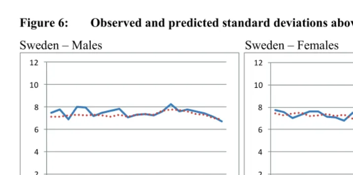
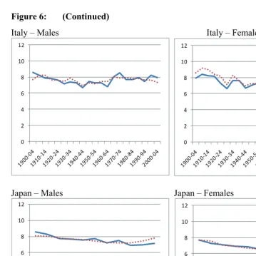
The series for the observed and predicted values of SD(M+) are illustrated in Figure 6. Considering that these two series are derived so differently, and that all the points are independent, the agreement between the two series is very close.
Figure 6 clearly supports the basic conclusion that the prediction method works well enough to confirm the theoretical deduction from the model: that e(M) and SD(M+) can be predicted from the death rates at just two high ages, such as 70 and 90. In order fully to understand the changes in e(M) and SD(M+), we need to understand the factors which affect the death rates at these ages.
Figure 6: Observed and predicted standard deviations above the mode
Sweden – Males Sweden – Females
0 2 4 6 8 10 12
0 2 4 6 8 10 12
Switzerland – Males Switzerland – Females
0 2 4 6 8 10 12
0 2 4 6 8 10 12
Figure 6: (Continued)
Italy – Males Italy – Females
0 2 4 6 8 10 12
0 2 4 6 8 10 12
Japan – Males Japan – Females
0 2 4 6 8 10 12
0 2 4 6 8 10 12
Plain line is Observed SD(M+); Dotted line is Predicted SD(M+).
Figure 6: (Continued)
England & Wales – Males England & Wales – Females
0 2 4 6 8 10 12
0 2 4 6 8 10 12
France – Males France – Females
0 2 4 6 8 10 12
0 2 4 6 8 10 12
5. Discussion
The previous section concluded that in the six countries studied, there had been mortality compression above the mode in the period from 1950-1954 to 2000-2004. The fall in the observed SD(M+) for females was an average of 1.3 years, but 1.8 in Sweden and 1.6 in Japan. This differs from one of the conclusions found by Bongaarts (2005). He used the 3-parameter logistic model, which includes Makeham’s constant taken as a measure of “background mortality”. When this model was fitted to ages 25-109, he found that in many countries the parameter b had remained almost constant from 1950 to 2000. He therefore decided that it was reasonable to assume that in future the parameter b would remain constant over time for any given country. This means that the frequency distribution of ages at death will shift to the right without any change of shape or compression above the mode. This is the shifting logistic model.
A key reason for the difference between these two conclusions is the fact that Bongaarts fitted his model to the very wide range of ages from 25 to 109, whereas we only used data at ages 70 and over. Bongaarts (2008) has since found that if his model is fitted over shorter age ranges, the estimates of the slope b are not all the same. In particular, if the model is fitted to ages 30-109 then b appears almost constant over time, whereas if the same model is fitted to ages 70-90 and 70-109 there is a marked increase in b over time. This is fully consistent with Kannisto’s finding, and ours, about the mortality compression above the mode. A further factor may be that the slope b which fits the ages below 70 has not remained the same as the slope which fits ages 70 and over. In this paper, we have confined ourselves to ages 70 and over.
Kannisto (2001) has shown that that SD(M+) fell for some female populations in recent decades. In order to study this mortality compression further, we combined Kannisto’s measures with the simple two-parameter logistic model. Our results support Kannisto’s extended to cover males as well as females and also the most recent periods. Kannisto contended that the compression he observed was due to the resistance caused by the ascending trajectory of mortality. In our analysis, the resistance is reflected in the fact that the death rates at very high ages did not fall fast enough to prevent compression. This is a distinction without much of a difference.
The compression above the mode, however, has been fairly slow, and it is an open question how far SD(M+) may continue to fall. Nevertheless, if medical advances do not have quite the same effect around age 90 as around age 70, the compression may continue to hold for some time yet. For the future, there is also the uncertainty that there may not be enough caregivers to look after the expected enormous numbers of old people. This may eventually affect the mortality rates of the very old.
6. Acknowledgments
References
Beard, R.E. (1971). Some aspects of theories of mortality, cause of death analysis, forecasting and stochastic processes. In: Brass, W. (ed.). Biological Aspects of Demography. London: Taylor and Francis: 57-68.
Bongaarts, J. (2005). Long-range trends in adult mortality: models and projection methods. Demography 42(1): 23-49. doi:10.1353/dem.2005.0003.
Bongaarts, J. (2008). [Private communication between April 17- May 5 2008. Available on request from the authors; contact Siu Lan K. Cheung at [email protected]].
Canudas-Romo, V. (2008). The modal age at death and the shifting mortality hypothesis. Demographic Research 19(30): 1179-1204. doi:10.4054/DemRes. 2008.19.30.
Canudas-Romo, V. (2010). Three measures of longevity: time trends andrecord values.
Demography 47(2), forthcoming.
Cheung, S.L.K., Robine, J.-M., Tu, E.J.C., and Caselli, G. (2005). Three dimensions of the survival curve: horizontalization, verticalization, and longevity extension.
Demography 42(2): 243-258. doi:10.1353/dem.2005.0012.
Cheung, S.L.K. and Robine, J.-M. (2007). Increase in Common Longevity and the Compression of Mortality: The case of Japan. Population Studies 61(1): 85-97.
doi:10.1080/00324720601103833.
Cheung, S.L.K., Robine, J.-M., and Caselli, G. (2008). The use of cohort and period data to explore changes in adult longevity in low mortality countries. Genus
LXIV(1-2): 101-129.
Cheung, S.L.K., Robine, J.-M., Paccaud, F., and Marazzi, A. (2009). Dissecting the compression of mortality in Switzerland, 1876-2005. Demographic Research
21(19): 569-598. doi:10.4054/DemRes.2009.21.19.
Comfort, A. (1956). The biology of senescence. Frome and London: Butler & Tanner Ltd.
Fries, J.F. (1980). Aging, Natural Death, and the Compression of Morbidity. The New England Journal of Medicine 303(3): 130-135.
Human Mortality Database (2007). Human Mortality Database [electronic resource]. Berkeley: University of California, and Rostock: Max Planck Institute for Demographic Research. http://www.mortality.org/
Kannisto, V., Lauristen, J., Thatcher, A.R., and Vaupel, J.W. (1994). Reductions in mortality at advanced ages: several decades of evidence from 27 countries.
Population and Development Review 20(4): 793–809. doi:10.2307/2137662. Kannisto, V. (1992). Presentation at a workshop on “Old age mortality” held at Odense
University, Odense, Denmark, June 1992.
Kannisto, V. (2000). Measuring the Compression of Mortality. Demographic Research 3(6). doi:10.4054/DemRes.2000.3.6.
Kannisto, V. (2001). Mode and dispersion of the length of life. Population: An English Selection 13(1): 159-171.
Le Bras, H. (1976). Lois de mortalité et âge limite. Population 3:655-691.
Lexis, W. (1878). Sur la durée normale de la vie humaine et sur la théorie de la stabilité des rapports statistiques. Annales de Démographie Internationale 2(5): 447-460. Pollard, J.H. (1991). Fun with Gompertz. Genus XLVII(1-2): 1-20.
Robine, J.-M., Cheung, S.L.K., Thatcher, A.R., and Horiuchi, S. (2006). What can be learnt by studying the adult modal age at death? Paper presented at PAA 2006 Annual Meeting, Los Angeles, United States of America, March 30-April 1 2007.
Strehler, B.L. and Mildvan, A.S. (1960). General theory of mortality and aging.
Science 132(3418): 14-21. doi:10.1126/science.132.3418.14.
Thatcher, A.R. (1999). The long-term pattern of adult mortality and the highest attained age. Journal of the Royal Statistical Society (A) 162 (Part 1): 5-43.
doi:10.1111/1467-985X.00119.
Thatcher, A.R., Kannisto,V., and Vaupel, J.W. (1998). The force of mortality at ages 80 to 120. Odense: Odense University Press (Monographs on Population Aging 5). Vaupel, J.W., Manton, K.G., and Stallard, E. (1979). The impact of heterogeneity in
individual frailty on the dynamics of mortality. Demography 16(3): 439-54.
doi:10.2307/2061224.
Wilmoth, J.R. and Horiuchi, S. (1999). Rectangularization Revisited: Variability of Age
at Death Within Human Populations. Demography 36(4): 475-495.
Yashin, A.I., Vaupel, J.W., and Iachine, L.A. (1994). A duality of aging: the equivalence of mortality models based on radically different concepts.
Mechanism of Ageing and Development 74: 1-14. doi:10.1016/0047-6374(94)90094-9.
Yashin, A.I., Begun, A.S., Boiko, S.I., Ukrainseva, S.V., and Oeppen, J. (2001). The New Trends in Survival Improvement Require a Revision of Traditional
Gerontological Concepts. Experimental Gerontology 37(1): 157-167.
doi:10.1016/S0531-5565(01)00154-1.
Yule, G.U. and Kendall, M.G. (1950). An introduction to the theory of statistics.
Appendix
Note: In this Appendix the symbols typed as µx and µ(x) are interchangeable, and similarly for other suffixes.
A1. M, e(M), and SD(M+) for a continuous distribution
Consider the case in which the ages at death have a continuous frequency distribution, with a density function d(x) which is estimated from data or which has been assumed to follow a mathematical equation that has been fitted to data by some suitable method. The adult modal age of death M is the age at which d(x) has its maximum in the age range defined as “adult age” (e.g., 15 and over). The remaining expectation of life for those who have just reached the mode is
( )
∫
∫
∞ ∞ − = M M dx x d x d M x M e ) ( ) ( ) ( dx (A.1)The standard deviation SD(M+) of the ages at death above the mode, measured from the mode, is
( )
∫
∫
∞ ∞ − = + M M dx x d x d M x M SD ) ( ) ( ) ( 2 dx (A.2)A2. Approximations when the distribution is discrete
In order to use the approximate formula, we must find in the life table the age X which has the highest number of deaths. We then extract the values of d(X), d(X-1) and d(X+1) as given in the life table. The approximate value of the mode is then given by
]
[
( ) ( 1)] [
( ) ( 1)) 1 ( ) (
+ − + − −
− − +
=
X d X d X d X d
X d X d X
M
(A.3)
This is the formula used by Kannisto (2001). It can be derived by the method of differences (see Yule and Kendall, 1950, page 582). It has also been derived from first principles by Canudas-Romo (2008). The tip of the continuous curve is approximated in the range (X-1, X+1) by the parabola which has the right areas below it to produce the observed values d(X-1), d(X) and d(X+1). The resulting estimate M always lies between X and X+1.
Having found an estimate of M, either by using (A.3) or in some other way, the expectation of life at the mode can be found by interpolating between the life table values e(X) and e(X+1). This gives
e(M) = e(X)*(X+1-M) + e(X+1)*(M-X). (A.4)
We now use the fact that the ratio of SD(M+) to e(M) is practically constant. In a Lexis model the ratio is always exactly 1.253. In the simple logistic model it is very slightly less, but in a very narrow band. Table 1 shows that the ratio lies between 1.231 and 1.235 when the parameter b lies anywhere from 0.09 to 0.15. For practical purposes we estimate SD(M+) by
SD(M+) = 1.233*e(M). (A.5)
A3. Different versions and derivations of the logistic model
The logistic model of mortality has been published in several different forms and notations, but all can be converted to the expression
μ (x) = c + kz / (1 + z) where z = aebx (A.6)
adult ages from causes which are not related to age. However, the presence of the denominator bends the curve downwards at high ages.
A very common explanation of this downward bend is that it can be caused by heterogeneity (selective survival). Because less healthy individuals are more likely to die at younger ages, survivors to older ages tend to have favourable health endowments and/or healthy life styles. This selection process could slow down the age-related mortality increase at the population level.
Specific assumptions about the nature of heterogeneity which lead to the expression (A.6) were first proposed by Beard (1971) and later discovered independently by Vaupel et al. (1979). Individual differences are assumed to remain essentially unchanged throughout their lifetimes, so the models are called the “fixed frailty” models, and the individual differences are assumed to follow the gamma distribution. However, it was also shown by Le Bras (1976) that the same expression (A.6) can be produced in a completely differently way, in which ageing is modelled as a stochastic process. Individuals progress by jumps at random times through a succession of steadily deteriorating states of health. Even a cohort which starts as homogeneous will become increasingly heterogeneous. Thus, completely different underlying mechanisms could produce the logistic pattern of mortality (Yashin et al. 1994).
The model (A.6) was among those fitted by Thatcher et al. (1998), though in a different notation, to all officially published data on deaths at ages 80 and over for males and females in 13 countries with reliable data for the ten-year periods from 1960-1990 and also for some cohorts in those countries. They found that at these ages c was negligible, of the order of 0.00001. This was surprising, as one would expect background mortality to extend to all ages. Presumably at ages 80 and over risks of death from most causes, even accidents, may be correlated with age. The parameters which they fitted showed that k was close to unity. This would also have been surprising, except for the fact that the combination c=0 and k=1 leads immediately to the logit relationship (3), which was already known to fit the data at high ages.
However, Thatcher (1999) realised that it was not possible to fit the two-parameter version of (A.6), with c=0 and k=1, to data extending down to age 30. He therefore tried the three-parameter version, taking k=1 but with no constraint on c. For the data from age 30 upwards the fitted value of c was of the order of 0.01, which is far from negligible as a component of an age-specific death rate. This shows that the 2-parameter model breaks down at some stage below age 80, when c ceases to be negligible. Moreover, Bongaarts (2008) has found that the slope b which fits the ages below 70 has not remained the same as the slope which fits ages 70 and over.
observation, which fortunately enables us to make the predictions of M and SD(M+) which are the subject of the paper.
A4. Proof of equation (4)
The force of mortality is defined as
dx x l d x l x ( )
) (
1 ) ( =−
μ
(A.7)
where l(x) is the life table survival function at age x.
The density of deaths at age x is given by
d(x) = l(x)µ(x) (A.8)
The mode of the distribution of deaths is therefore found by differentiating (A.8) and equating to zero. Substituting from (A.7) then produces
(dµx /dx) / µx = µx at the mode, i.e., for x = M. (A.9)
This is a standard result which applies to all continuous laws of mortality. Note that the left hand side of the above equation is the life table aging rate (LAR). Thus, at the modal age, the force of mortality is equal to the LAR. This important fact was previously shown by Pollard (1991) for the Gompertz model and by Robine et al. (2006) in a general form.
The simple logistic model is defined by equation (1) in the text. Differentiating µx with respect to x gives (dµx /dx) as a function of a and b. On substituting (A.9) the equation simplifies to produce
aebx = b at the mode, (A.10)
A5. Proof that in the simple logistic model, e(M) and SD(M+) are
determined solely by b, independently of M
In the simple logistic model, mortality above M is given by
by bM by bM y M b y M b y
M ae e
e ae ae ae + = + = ++
+ 1 ( ) 1
) (
μ for any y≥ 0
Substituting aebM=b from (A.10) into the above, we get
b by by by be dx d be be y
M ln(1 )1/
1 ) ( = + + = + μ (A.11) Thus,
[
]
{
}
bbx x y y b by x be b be dy y M M l x M l 1 0 / 1 0 1 1 ) 1 (ln( exp ) ( exp ) ( ) ( ⎟ ⎠ ⎞ ⎜ ⎝ ⎛ + + = + − = ⎟ ⎟ ⎠ ⎞ ⎜ ⎜ ⎝ ⎛ + − = + = =
∫
μ . (A.12)Therefore, the expectation of life at M, which is also the upward mean deviation of age at death from M, is given by
dx be b dx be be be b x dx x M M l x M l x M l dx x M xd dx x M d dx x M xd M e b bx by by b bx
∫
∫
∫
∫
∫
∫
∞ ∞ ∞ ∞ ∞ ∞ ⎟ ⎠ ⎞ ⎜ ⎝ ⎛ + + = + ⎟ ⎠ ⎞ ⎜ ⎝ ⎛ + + = + + = + = + + = 0 1 0 1 0 0 0 0 1 1 1 1 1 ) ( ) ( ) ( ) ( ) ( ) ( ) ( ) ( μ. (A.13)
by integration by parts. This clearly indicates that e(M) is solely determined by b, regardless of a and M.
Similarly, x d be be be b x dx M l x M l x M SD bx bx b bx x M
∫
∫
+ ∞ ∞ + ⎟ ⎠ ⎞ ⎜ ⎝ ⎛ + + = + = + 0 1 2 0 2 1 1 1 ) ( ) ( )( μ , (A.14)
A6. Proof of equation (10)
From equation (4) we have
ln a + bM = ln b
and hence, as in equation (6),
M = (ln b)/b – (ln a)/b (A.15)
In the simple logistic model, if µ(x1) is the force of mortality at any given age x1, then by equation (3) we have
a* = ln a = logit µ(x1) - bx1 (A.16)
Thus from (A.15)
M = (ln b)/b - [logit µ(x1)]/b + x1 (A.17)
Since m(x)’s, but not µ(x)’s, are given in empirical life tables, we can make use of the fact that m(x) is approximately equal to µ(x + ½). Hence, using equation (3), we find
logit m(x) = logit µ(x+1/2) = logit µ(x) + b/2 (A.18)
Substituting (A.18) into (A.17) gives
M = (ln b)/b - [logit m(x1)]/b + x1 + ½ (A.19)