DEMOGRAPHIC RESEARCH
VOLUME 29, ARTICLE 22, PAGES 579-616
PUBLISHED 26 SEPTEMBER 2013
http://www.demographic-research.org/Volumes/Vol29/22/ DOI: 10.4054/DemRes.2013.29.22
Research Article
Validation of spatially allocated small area
estimates for 1880 Census demography
Matt Ruther
Galen Maclaurin
Stefan Leyk
Barbara Buttenfield
Nicholas Nagle
© 2013 Ruther, Maclaurin, Leyk, Buttenfield & Nagle.
This open-access work is published under the terms of the Creative Commons Attribution NonCommercial License 2.0 Germany, which permits use, reproduction & distribution in any medium for non-commercial purposes, provided the original author(s) and source are given credit.
1 Introduction 580
2 Background 582
2.1 Small area estimation using Census microdata 582 2.2 Maximum entropy microdata allocation 583 2.3 The context of the 1880 Census 585
3 Methods 587
3.1 Finding meaningful constraining variables 587 3.2 Establishing a validation procedure 588
3.2.1 Error in margin 589
3.2.2 Residuals and Standardized Allocation Error (SAE) 589
3.3 Modified z-statistic 590
4 Results 591
4.1 The selection of constraining variables 591 4.2 Post-allocation results: Comparison of allocated distributions to
actual distributions
595
4.3 Post-allocation results: Comparison of the joint distribution of a constraining variable and a non-constraining variable
599
4.4 Post-allocation results: Comparison of the joint distribution of two non-constraining variables
600
4.5 Post-allocation results: Geographic heterogeneity in benchmark variable allocation errors
602
5 Discussion and concluding remarks 607
5.1 Limitations and future steps 611
6 Acknowledgement 611
References 612
Validation of spatially allocated small area estimates for 1880
Census demography
Matt Ruther1
Galen Maclaurin 2
Stefan Leyk2
Barbara Buttenfield2
Nicholas Nagle3
Abstract
OBJECTIVE
This paper details the validation of a methodology which spatially allocates Census microdata to census tracts, based on known, aggregate tract population distributions. To protect confidentiality, public-use microdata contain no spatial identifiers other than the code indicating the Public Use Microdata Area (PUMA) in which the individual or household is located. Confirmatory information including the location of microdata households can only be obtained in a Census Research Data Center (CRDC). Due to restrictions in place at CRDCs, a systematic procedure for validating the spatial allocation methodology needs to be implemented prior to accessing CRDC data.
METHODS
This study demonstrates and evaluates such an approach, using historical census data for which a 100% count of the full population is available at a fine spatial resolution. The approach described allows for testing of the behavior of a maximum entropy imputation and spatial allocation model under different specifications. The imputation and allocation is performed using a microdata sample of records drawn from the full 1880 Census enumeration and synthetic summary files created from the same source. The results of the allocation are then validated against the actual values from the 100% count of 1880.
1 University of Colorado Boulder, U.S.A. E-mail: [email protected]. 2
University of Colorado Boulder, U.S.A.
RESULTS
The results indicate that the validation procedure provides useful statistics, allowing an in-depth evaluation of the household allocation and identifying optimal configurations for model parameterization. This provides important insights as to how to design a validation procedure at a CRDC for spatial allocations using contemporary census data.
1. Introduction
Census public-use microdata possess an attribute richness which should make them tremendously useful to researchers interested in demographic small area estimation; however, they are underutilized, largely due to their coarse spatial resolution. The smallest identifiable geographic areas in Census microdata contain a minimum of 100,000 individuals, a restriction which may significantly compromise the geographic nature of a demographic study. Research which focuses on smaller geographic areas generally relies on a limited number of aggregate population characteristics provided by the Census Bureau in summary tables and cross-tabulations at the census tract or block group level. In order to better exploit the attribute richness of Census microdata at finer spatial scales, spatial allocation methods, which allocate microdata households to small areas and generate summary statistics for these smaller geographic units using the attributes of the allocated microdata households, may be used (Johnston and Pattie 1993; Ballas et al. 2005; Assunção et al. 2005). Small area estimates, which contain extensive detail on the underlying population, are in great demand and are important to research on demographic and social processes such as migration, impoverishment, and human-environmental interactions.
A persistent shortcoming in the use of such spatial allocation methods for deriving demographic small area estimates is the lack of confirmatory validation. There are often few, if any, sources against which to compare the estimated fine-scale population counts and the associated distributions of population characteristics. The main reason for the absence of fine-resolution comparison data is the confidentiality protection in census surveys, which precludes the release of confirmatory data. Although demographic estimates based on U.S. Census data and geographies may be validated at a Census Research Data Center (CRDC), the expense of accessing a CRDC and the necessary confidentiality restrictions in place at the CRDC mandate that the validation process, which is not trivial, be fully realized prior to its implementation at the CRDC.
set of (different) target zones. The estimation methodology used here was originally developed to spatially allocate Public Use Microdata Sample (PUMS) households, which are spatially contained within Public Use Microdata Areas (PUMAs) (source), to census tracts (target), by imputing tract-specific sampling weights for each microdata household. The imputation is based on the principle of maximum entropy: Conditional on prior information known about the data, the most uniform distribution (i.e., all values have equal probability of occurrence) best represents the data-generating process (Phillips, Anderson, and Schapire 2006). Maximum entropy models are constrained by the information that is known about the process while making no assumptions about what is unknown. In this case, the model maximizes uniformity of the distribution of tract-specific sampling weights, subject to the constraint that the weights sum to the known, aggregate tract populations (summary statistics) (Nagle et al. 2013; Leyk, Buttenfield, and Nagle 2013).4
The fine-scale data necessary for the validation of this methodology for contemporary Censuses are available only at a CRDC. In contrast, historical Census data from 1880 are publicly available, and these data contain the full demographic detail for a 100% count of the population.5 This historical data is used to (1) generate a nested data structure comparable to contemporary census data (i.e., a 5% microdata sample and small area population summary statistics), (2) run the imputation model and allocate households based on the imputed weights, and (3) examine and validate model performance.
In the context of methodological validation, the 1880 Census presents a unique opportunity, as the publicly available data include the full count of the population at a fine spatial resolution. The spatial structure of the 1880 Census data is comparable, although not identical, to that of contemporary censuses, and the collected population
4
Although originally developed and tested for the U.S. context using PUMAs and census tracts, the allocation method described in this paper could conceivably be carried out using data from other nations. The international version of the Integrated Public Use Microdata Series (IPUMS), maintained by the Minnesota Population Center (MPC), includes microdata from many countries, and national statistical agencies frequently provide aggregate population data for small sub-national geographies. The applicability of the method described here to an international context will depend on the unit of microdata geography and the unit of aggregate population geography used in a particular country. In the U.K., for example, the Sample of Anonymised Records microdata regions are quite similar in size to PUMAs in the U.S., and the Output Areas (the smallest geography for which U.K. aggregate population estimates are made) are comparable to U.S. census tracts. In other countries (e.g., France and Germany), the smallest geographical unit identified in the microdata (German states or French regions) is considerably larger than a PUMA; the spatial allocation may not perform adequately in these cases.
5 In fact, historical records from U.S. Censuses in 1940 and decades prior are publicly available and preserved
characteristics are similar. Thus the performance of spatial microdata allocation procedures can be objectively evaluated and interpreted to better understand the quality of finer resolution demographic estimates and how they reflect underlying population characteristics when the model parameters are changed. In order to mimic the data available in contemporary censuses, a random 5% sample of population is drawn from the full 1880 Census enumeration (comparable to current PUMS data) and “synthetic” summary tables are created from the same source (comparable to SF3 files). The spatial allocation procedure will be performed on these historical data using different combinations of constraining variables, and the results will be validated against the actual values from the 100% population count.
The primary purpose of this article is to evaluate the performance of a spatial allocation model which generates small area estimates, through comparisons of these estimates with actual population counts and an investigation of model residuals and their geographic variation. The paper will also shed light on the evaluation process itself, highlighting important considerations in parameter selection and their influence on resulting estimates for different population attributes. These considerations are crucial in designing a robust validation process prior to undertaking the validation of the allocation results using contemporary census data at a CRDC. Data from the 1880 Census are utilized here as an easily accessible and appropriate surrogate for contemporary census data; as such, the priority in this analysis is neither in historical interpretations of these allocation results nor in drawing substantive conclusions regarding demographic processes in 1880. This article focuses on confirmatory testing that can be directly reproduced using contemporary public-domain Census data, as well as confidential data in a CRDC, and provides preliminary validation measures for spatial allocation methods.
2. Background
2.1 Small area estimation using Census microdata
of synthetic or reweighted microdata (Williamson, Birkin, and Rees 1998; Voas and Williamson 2001). A general shortcoming in validating the performance of such models is the lack of a “true” population against which the allocation results can be compared. Beckman, Baggerly, and McKay (1996) apply an iterative proportional fitting (IPF) technique to 1990 U.S. Census data and demonstrate that estimated tract-level household distributions are concordant with tract-level summary statistics released by the Census Bureau. However, they validate their estimates against a different sample drawn from the same population, not against the 100% population count. Melhuish, Blake, and Day (2002) use a reweighting process that allocates Australian household survey data which lack locative information to small census districts based on the known sociodemographic profiles of these small geographies. Their evaluation of the results suggests that the allocated populations correctly match the 100% population counts for most districts, but data to evaluate the joint distributions for most population characteristics are not publicly available. Hermes and Poulsen (2012) provide a current and general overview of the use of microdata reweighting techniques in generating small area estimates.
2.2 Maximum entropy microdata allocation
A methodology to allocate reweighted demographic microdata to small enumeration areas such as census tracts using decennial U.S. Census data has been recently described (Nagle et al. 2012; Leyk, Buttenfield, and Nagle 2013), based on the concepts of dasymetric mapping and areal interpolation (Mrozinski and Cromley 1999). In this approach, maximum entropy methods impute a set of tract-specific sampling weights for each microdata record, with the initial tract-specific weights derived from the survey design weight. The imputed weights are constrained to match the known (i.e., publicly available) tract-level distributions for a number of population characteristics; the weights imputation is thus guided and influenced by this chosen set of constraining variables. Sampling weights for each microdata household sum across all tracts to the approximate design (or household) weight provided by the Census Bureau. As the design weight reflects the expected number of households in the Public Use Microdata Area (PUMA) that are similar to a given microdata record, each constructed sampling weight can be interpreted as the number of households of this “type” that can be expected in the respective census tract.
population has attributes similar to those of PUMS household i and is located in census tract j, it is possible to impute the k-th tract-level attribute value by the equation
∑ . At the outset of modeling, the probabilities pij are unknown. The imputation is constrained such that the imputed probabilities reproduce tract-level populations given in Census summary files:
∑ ∑ ( ) (
) (1)
subject to ∑ and ∑
for all households i, tracts j, and attributes k. The yjk are tract-level summaries of attribute k from the summary files, and dijare prior estimates of tract-level (i.e., for each tract j) weights for each PUMS record i, which are subject to reweighting (Leyk, Buttenfield, and Nagle 2013). Following the maximum entropy imputation, the set of imputed weights guides allocation of households to individual tracts or other sub-PUMA areas.
Although maximum entropy imputation is but one of many methods through which this type of data imputation or reweighting may be performed, it offers certain advantages. The tract-specific weights imputed through maximum entropy will not lead to negative population estimates, as can be the case with least squares regression techniques, and the reweighted tract population distributions for constraining variables will exactly reproduce those distributions in the summary tables. The maximum entropy procedure used here also retains, for each microdata record, the full set of attributes present in the record, allowing for the construction of revised summary tables for every available attribute or combinations of attributes.
Once allocated, the microdata household characteristics can be summarized to (1) create revised estimates of tract-level (or finer-scale) demographic summary statistics, (2) generate summary statistics of attributes not available in summary files, and (3) compute new cross-tabulations. In Leyk, Buttenfield, and Nagle (2013), the revised summary statistics were compared to original tract population distributions from the Census-produced summary tables (based on a 1-in-6 sample), and allocation ambiguity was evaluated for each household as a function of the distribution of imputed sampling weights over all census tracts. While correlations between the revised tract-level summaries and original tract summary statistics were found to be high and statistically significant for constraining and non-constraining variables, a full validation could not be conducted without access to the full population details maintained at a CRDC.
allocated to enumeration districts according to their exact imputed sampling weights. From these allocations, revised summary statistics are computed for each enumeration district. These revised tables are then compared against the true aggregated population attributes from the full (100%) population count. While the maximum entropy imputation model detailed above is explored here, any allocation model that uses similar demographic data could be validated using the procedure outlined in this paper.
2.3 The context of the 1880 Census
The 1880 Census is considered the first high-quality enumeration of the U.S. population and full individual records from this historical census have been digitally transcribed and made available online (Goeken et al. 2003; Ruggles et al. 2010). Important for the research reported here, the 1880 Census records contain household microdata including spatial identifiers for the geographic units – enumeration districts – in which the households were located as well as the spatial boundaries of these districts. Although neither PUMAs nor census tracts had yet been defined in 1880, State Economic Areas (SEAs) and enumeration districts (EDs) represent a similar spatial data structure as can be found in contemporary censuses. SEAs, which consist of single counties or groups of contiguous counties, were defined for the 1950 Census and retroactively applied to prior censuses by the Minnesota Population Center (Bogue 1951; Ruggles et al. 2010). SEAs were designed to have a minimum population of 100,000 people, much like contemporary PUMAs, although the retrospective definition of SEAs to the 1880 Census may result in substantially different population sizes. SEAs were divided into minor subdivisions known as EDs, similar to contemporary census tracts but slightly smaller; these districts corresponded to the area that a door-to-door enumerator could cover during the Census period. EDs are fully nested in and completely enclosed by SEAs. The similarity between SEAs and PUMAs, and EDs and census tracts, allows the 1880 Census to serve as a reasonable substitute for more current censuses in performing and validating the allocation method.
Because the number of observed attributes found in each individual record is quite large, the validation and discussion of the spatial allocation results will focus on selected benchmark variables commonly used by, and of particular interest to, demographic researchers. These benchmark variables include the gender, age, race, and marital status of the householder; the full list of benchmark variables and their categorizations are shown in Table 1.
Table 1: Benchmark variables for validation of spatial allocation validation
Benchmark
Number of categories
Measurement Record Count
(PUMS N = 3,408)
Age of Householder 4 Age 0-17 87
Age 18-34 976
Age 35-49 1,278
Age 50+ 1,067
Gender of Householder 1 Male 2,747
Race of Householder 1 Non-White 151
Marital Status of Householder 2 Single 305
Married 2,542
Presence of Children in Household 2 Any Children 2,528
5+ Children Present 555
Nativity of Householder1 2 Native Born 872
Foreign Born 1,918
Occupational Status of Householder2 4 Non-Worker 637
Low-Skill 997
Medium-Skill 909
High-Skill 865
Group Quarters Status of Household3 1 Group Quarters 293
Urban Status of Household4 1 Urban Household 2,788
Farm Status of Household 1 Farm Household 219
Notes: 1 Native born refers to individuals born in the U.S. with parents who were born in the U.S. Foreign born refers to individuals not born in the U.S. A third grouping, U.S.-born household heads whose parents were foreign born, is not considered here.
2
Occupational standing is measured using the occupational earnings score variable, with the observed variable broken into three tertiles (Low-Skill, Medium-Skill, and High-Skill). Non-workers were individuals outside of the labor force.
3
Because households were not defined in the 1880 Census, the contemporary distinction between group quarters and households is not relevant here.
4
The converse of “Urban” is “Rural”, distinct from but correlated with the “Farm” designation.
used as constraining variables in the allocation procedure, the function of the remaining benchmark variables is to serve as validation instruments.
3. Methods
The 1880 Census data were used to run the weights imputation and spatial allocation model for Hamilton County, Ohio. This county was chosen based on its stable boundaries over time and the fact that it was coextensive with a single SEA (SEA 336). Although the 1880 Census did not define households in the same way as is done in contemporary Censuses, variables describing household composition were added retrospectively during data transcription (Goeken et al. 2003; Ruggles et al. 2010). There were 68,160 households (comprising 313,702 individuals) in Hamilton County in the 100% count of the 1880 Census. Household characteristics were identified using the records for all individuals listed as person number one (head of household), and all references to household or householder refer to the attributes of this individual. Individuals living in group quarters, who are not considered household members in current Censuses, are considered household members in this study. Hamilton County was divided into 135 EDs, which contained, on average, 505 households (or approximately 2,300 individuals). A 5% sample, similar to a contemporary PUMS, was randomly drawn from the full count of households in the SEA, and each household in this sample was assigned a design weight (household weight) of 20. This “pseudo-PUMS” (N=3,408) comprises the analytical sample used in the maximum entropy procedure, which is subsequently spatially allocated among the 135 EDs covering the county.
Prior to running the weights imputation, a crucial task is the selection of constraining variables; this procedure is described first. Then three different measures are described that can be used to validate the imputation and allocation results for different combinations of constraining variables. As noted above, this study focuses on the validation procedure; technical details about the maximum entropy weights imputation and allocation model beyond the above summary are described in Nagle et al. (2012; 2013) and Leyk, Buttenfield, and Nagle (2013).
3.1 Finding meaningful constraining variables
Population characteristics (such as gender) that are similarly distributed among EDs are unlikely to produce satisfactory allocation results when used as constraints, since there may be little variation to exploit. In addition, the inclusion of multiple highly correlated variables may be unnecessary, as highly correlated variables will likely be redundant in explaining variation in the underlying population distribution. The choice of constraining variables represents a difficult problem in survey sampling that has found limited attention to date and there is no standard method in place.
Bivariate correlations of ED-level population characteristics are calculated as one obvious way of assessing highly correlated variables that would be unsuitable constraining variables if applied in concert. Principal component analysis (PCA) is used to examine how much variation in the data is explained by the different population characteristics, and thus to identify the variables that may be most useful as constraints. While PCA is commonly used to reduce the dimensionality in a given set of data, it may also be helpful in describing the associations between the variables present in the data (Jolliffe 2002; Demšar et al. 2013). Finally, a segregation index, the index of dissimilarity (D), is computed at the ED-level to determine those variables that may represent appropriate constraints. The index of dissimilarity is a measure of the evenness of the distribution of two groups (Massey and Denton 1988), and may therefore be helpful in determining which variables best differentiate (or segregate) household residential patterns. Dissimilarity index values range from 0 to 1, with values tending towards 1 indicative of more highly segregated groups and values tending towards 0 suggesting low levels of segregation among the groups.
3.2 Establishing a validation procedure
constraining variable. An important component of the validation task then is to establish how well the revised summary statistics for household attributes not used as constraints replicate the actual number of households with those attributes in each ED. Following each model run, revised summary tables were generated by ED for the attributes of interest (benchmark variables as described above) based on the allocated microdata. The revised summary tables were compared to summary tables constructed from the 100% enumeration of the population. To examine the accuracy of allocation results from different perspectives, three goodness-of-fit statistics were calculated, as described below.
3.2.1 Error in margin
The actual number of households in the entire study area exhibiting a particular population characteristic will be compared to the total allocated number of households with the same characteristic in order to assess how well individual variables are being allocated overall; this difference is designated the error in margin. While the error in margin reveals little about the performance of the allocation procedure in reproducing the accurate population distribution within EDs, substantial differences between total household counts and allocated household counts will indicate variables for which the model critically fails. In short, concordance between the total number of allocated households and the total number of actual households is a necessary, but not sufficient, condition under which to validate model performance.
Importantly for the implementation of the allocation model with current Census data, the error in margin can be easily calculated in most cases based on publicly available data, even for attributes for which the other goodness-of-fit statistics described below cannot be derived. In such cases it is important to examine how well errors in margin correspond to the standardized absolute error or z-statistics described below, which quantify the error in the distribution. These measures are sometimes irretrievable from contemporary censuses without access to confidential data.
3.2.2 Residuals and Standardized Allocation Error (SAE)
∑ | |
∑ (2)
where Uiis the actual count of the population in EDi and Ti is the allocated count of the population in EDi. SAE will generally fall between 0 and 2, with values closer to 0 indicating a better fit between the actual and allocated distributions. Because the allocated margin is not required to match the actual margin for non-constraining variables, the SAE could, in theory, be greater than 2 for these variables. The SAE compares the actual ED-level household distribution to the allocated ED-level household distribution, and is a stricter evaluation of the accuracy of the model than is the error in margin described above; SAE is thus the primary measure of model performance. SAE is used to test the performance of a variety of model specifications (e.g., different variables used as constraining variables) and to compare across specifications. The SAE may also be computed for individual EDs, or for individual estimates within an ED. In this sense, the SAE is similar to a coefficient of variation, which is calculated as the standard error of an (average) estimate divided by the estimate itself.
3.3 Modified z-statistic
The modified z-statistic can be used to compare a table representing the actual joint distribution (or cross-tabulation) of multiple population attributes with a table representing the allocated joint distribution of those attributes (Williamson, Birkin, and Rees 1998). The z-statistic is calculated for each corresponding pair of table cells, with significant values representing those elements in the distribution of the particular population attribute for which the allocation procedure is performing inadequately. The modified z-statistic is calculated by
√
∑
∑
∑ (3)
The above three measures will highlight those variables which show unusual behavior within the allocation procedure and make it possible to carry out an in-depth validation based on the available full population count. Of particular interest is the level of accuracy with which non-constraining variables can be estimated. An important question is whether one can differentiate between those non-constraining variables which are strongly correlated with one or more constraining variables, and those which are seemingly unrelated to any of the constraining variables. This will provide important insight for the selection process of constraining variables and the configuration of the allocation model. The described validation procedure will also indicate whether the accuracies of the ED estimates for different population characteristics exhibit geographic heterogeneity through the compilation of residual maps, and whether the goodness-of-fit for an allocated distribution, as measured by the SAE, can be inferred from the error in margin.
The focus on these different measures of error, and the relationships between the measures, is based on the consideration that, in the contemporary context, model performance may need to be assessed under different conditions. The error in margin can be evaluated with no knowledge of the underlying tract-level distribution of the population and the data necessary to carry out this evaluation is frequently available in summary tables at the county- or PUMA-level. This is true even for those population attributes for which no census tract summaries are publicly available. However, the error in margin is limited in assessing model performance because it does not provide any information about the distributional accuracy of the model. The SAE and the modified z-statistics can be used to evaluate distributional accuracy, but can be calculated only when tract-level summary tables are available. Of course, this is not to say that the calculation of these latter measures requires the 100% count of the population that is available here; however, having the 100% count of the population allows SAE to be calculated for the full range of sociodemographic variables and, more importantly, for any cross tabulations of variables in the microdata.
4. Results
4.1 The selection of constraining variables
by the summary tables produced by the Census Bureau. As noted above, while the choice of constraining variables should be grounded in theory, there are analytical techniques that may guide the selection process. In this study segregation indices, bivariate correlations, and principal component analysis are used to determine favorable constraining variables i.e., variables with higher potential explanatory power that are not strongly correlated.
Table 2 displays the index of dissimilarity, measured at the level of the ED using the aggregate summary tables, for each of the benchmark variables. Some variables, including the urban/rural dichotomy, residence in group quarters, and farm residence, display very high levels of segregation, due to their natural geographical disparity. However, several benchmark variables are highly correlated, and the inclusion of multiple highly correlated variables as constraints would be redundant. Examples of highly correlated variables include urban residence and farm residence (Spearman ρ=-0.64) and group quarters status and single status (Spearman ρ=0.69). The full correlation matrix for all benchmark variables is displayed in Appendix 1.
Principal component analysis (PCA) provides another method of selecting relevant and non-superfluous constraining variables. The results from the PCA run on the ED-level aggregate summary tables for the 19 benchmark variables suggest that five underlying latent variables explain more than 85% of the variation in the benchmarks. These five principal components all have eigenvalues greater than 1; the sixth principal component has a substantially smaller eigenvalue.6
6
Table 2: Segregation indices for Hamilton County, Ohio (diversity measured by enumeration district)
Variable D
Urban vs. Rural 1.00
Farm vs. Non-farm 0.81
Group vs. Non-group 0.81
Male vs. Female 0.14
White vs. Non-white 0.53
Single vs. Non-single 0.25
Married vs. Non-married 0.13
Children present vs. No children present 0.13
5+ Children present vs. Less than 5 children present 0.15
Foreign born vs. Non-foreign born 0.28
Native vs. Non-native 0.39
Occupation: Non-worker vs. All other 0.13
Occupation: Low-skill vs. All other 0.27
Occupation: Medium-skill vs. All other 0.19
Occupation: High-skill vs. All other 0.14
Age: Age 0-17 vs. All other 0.76
Age: Age 18-34 vs. All other 0.07
Age: Age 35-49 vs. All other 0.06
Age: Age 50+ vs. All other 0.09
Note: The urban/rural dichotomy has an index of dissimilarity of 1 because EDs are wholly classified as either urban or rural, with the classification extending to all households within the district. While no such “perfect” constraining variables will exist in contemporary Census data, this variable was nevertheless retained as a constraint.
a constraining variable also allows for its use in the confirmatory validation that follows.
While the constraining variables used here are chosen through a quantitatively informed selection procedure, this procedure should not be construed as the de facto standard for choosing the “optimal” constraining variables for the model. There are variables available in the 1880 Census that are not considered in this paper, and the groupings of householder age and occupational status used here may not reflect the ideal categorizations for these variables. Cross-tabulations or interactions of individual variables (e.g. race by age, gender by occupational status) could also be constructed and used as constraints, in the hope that such interactions would ultimately provide improved estimates. However, the constraining variables selected above are assumed to be sufficiently robust for the validation procedure which follows.
As noted above, the primary purpose of this paper is to describe a method of validating small area estimates using perfect and complete census information and to infer from the validation results a process for validating when such complete information is not available. A second purpose, however, is to assess how changing estimation parameters affect model performance and the estimates themselves. To this end, while the model with five constraints will form the base model, models with 2-4 constraining variables will also be estimated. This step-wise modeling approach will facilitate the evaluation of the sensitivity of the estimation procedure to changes in the model parameterization. Because adding constraints is likely to increase the accuracy of the spatial allocation process in reproducing the actual 100% population distribution, a natural inclination would be to add constraining variables until the supply of available constraints was exhausted. However, overfitting of the maximum entropy model through the inclusion of an excessive number of constraining variables may lead to inefficiency and non-convergence. This may be particularly true in cases where the univariate or joint population distributions (such as summary statistics from the Census SF3 or American Community Survey) for constraint variables used in the maximum entropy imputation include sampling error or imputed data.
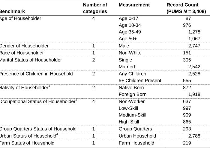
4.2 Post-allocation results: Comparison of allocated distributions to actual distributions
Figure 1 compares the total population counts in the SEA to the allocated population counts following the maximum entropy allocation model with five constraining variables. The variables used as constraints are listed first (within the gray area), followed by the additional benchmark variables. While the 100% population counts and the allocated population counts for constraining variables are, by design, the same, this chart highlights how the allocated total counts for the other benchmark variables are very close to their actual counts. For example, the actual number of male householders in Hamilton County is 54,932, while the number of male householders predicted by the model is only slightly larger, at 54,999.
The largest absolute errors in margin occur in the number of households with five or more children, for which 931 households are over-allocated (9.1% error in margin), and in the number of married householders, over-predicted by 589 households (1.2% error in margin). Other than the variable denoting married householders, the only benchmark variable with an error in margin greater than 5% is the number of householders younger than age 18 (6.5% error in margin).
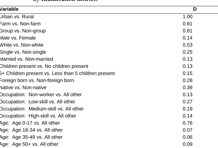
Figure 2 displays the SAE (distributional error) metrics for those benchmark variables not used as constraining variables in the five-constraint maximum entropy model; by design the SAE for variables used as constraints is 0. Although many of the benchmarks appear to be well allocated by this measure, two variables have noticeably poorer fits: Householders younger than age 18 and farm households. The SAE is equivalent to the mean residual divided by the mean actual number of households. On average, the number of allocated households in an ED is within approximately 20% of the actual number of households in that ED, for most benchmark variables.
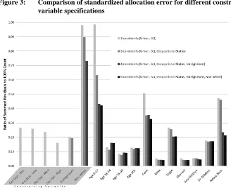
The maximum entropy procedure was also run with different numbers of constraining variables to evaluate how additional constraints affect the distribution of allocation errors. Figure 3 displays the SAEs of the benchmark variables for the maximum entropy models with 2-4 constraining variables, as well as the SAEs for the baseline five-constraint model. As before, these SAEs fall to zero when a variable is used as a constraint in the model. In general, the addition of constraining variables to the model reduces the SAE for the benchmark variables, although the magnitude of the decrease appears to depend on the relationship between the benchmark variable and the newly added constraint. For example, the error in the allocation of farm households drops substantially when occupational status is added as a constraining variable (most farm householders have low occupational status), while the error in the allocation of native-born households is greatly reduced when foreign-born is added as a constraint. Several benchmark variables, including those representing ages above 18, gender, and marital status, exhibit little change when additional constraints are added to the model. These benchmarks are largely uncorrelated with any of the constraining variables and generally have small errors under any of the model specifications.
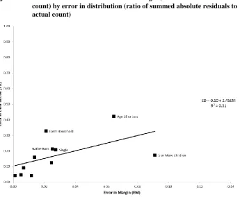
One final facet in the evaluation of model performance is the association between the error in margin and the SAE. Figure 4 highlights the relationships between the errors in margin of the benchmark variables (x-axis) and their ED-level SAE (y-axis), for the model with 5 constraining variables. A linear regression line is provided to summarize the point relationship between the two measures of error. The error in margin and the SAE exhibit a positive association, although it is fairly weak. Notably, the total allocated counts of both farm households and householders less than age 18 are very close to their actual counts in the population, but the distribution of these populations within specific EDs is much less successful. It appears therefore that inferences about the distributional performance of the allocation model based on agreement between the actual and allocated totals (error in margin) should be approached with caution. This underscores the earlier statement that the error in margin is itself insufficient in determining model performance.
4.3 Post-allocation results: Comparison of the joint distribution of a constraining variable and a non-constraining variable
To this point, only allocation errors in the univariate distributions of the group of benchmark variables have been explored. However, researchers are often interested in the joint distributions of variables; indeed, one anticipated goal from developing spatial allocation models using microdata is the ability to estimate joint distributions of variables for which none had previously existed. To assess the accuracy of the spatial allocation in duplicating the actual joint distributions of variables, the z-statistic described above may be used.
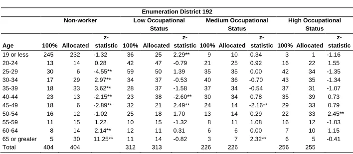
The top two panels of Table 3 display, for two randomly selected enumeration districts, the actual numbers of households, the allocated numbers of households, and the calculated z-statistics for the cross-tabbed distribution of a household attribute used as a constraining variable, householder occupational status, and a household attribute not used as a constraining variable, householder age. These tables reveal ED-specific discrepancies in the allocation performance of the model and may also highlight broad misallocation trends, such as that seen among the non-worker occupational class in both EDs. The last panel of Table 3 shows the aggregated performance metrics for each occupation/age group cell as the total number (and percent) of EDs which are well-allocated for that cell. In general, the number of well-well-allocated EDs is quite high for any particular cell, with noticeable patterns of poor allocation among the 25-29 age group and among the oldest householders.
Table 3: Comparison of allocated age and occupational status distribution to 100% count distribution
Enumeration District 192
Non-worker Low Occupational
Status
Medium Occupational Status
High Occupational Status
Age 100% Allocated
z-statistic 100% Allocated
z-statistic 100% Allocated
z-statistic 100% Allocated z-statistic
19 or less 245 232 -1.32 36 25 2.29** 9 10 0.34 3 1 -1.16
20-24 13 14 0.28 42 47 -0.79 21 25 0.92 16 22 1.55
25-29 30 6 -4.55** 59 50 1.39 35 35 0.00 42 34 -1.35
30-34 17 29 2.97** 34 37 -0.53 40 36 -0.70 43 35 -1.34
35-39 18 33 3.62** 28 37 -1.58 37 34 -0.54 37 31 -1.07
40-44 23 13 -2.15** 23 38 -2.60** 30 34 0.78 35 39 0.73
45-49 18 6 -2.89** 32 21 2.49** 24 14 -2.16** 29 33 0.79
50-54 16 12 -1.02 25 18 1.70 13 14 0.29 22 33 2.45**
55-59 11 15 1.22 10 15 -1.32 8 11 1.08 16 12 -1.03
60-64 8 14 2.14** 12 11 0.31 6 6 0.00 7 10 1.15
65 or greater 5 30 11.25** 11 14 -0.82 3 7 2.32** 6 5 -0.41
Table 3: (Continued)
Enumeration District 115
Non-worker Low Occupational
Status
Medium Occupational Status
High Occupational Status
Age 100% Allocated
z-statistic 100% Allocated
z-statistic 100% Allocated
z-statistic 100% Allocated z-statistic
19 or less 108 83 -3.60** 1 3 2.01** 0 0 0.00 0 2 2.00**
20-24 1 6 5.01** 5 4 -0.46 6 7 0.42 2 14 8.53**
25-29 2 5 2.13** 5 12 3.22** 9 16 2.42** 10 29 6.16**
30-34 2 15 9.24** 15 11 -1.13 32 21 -2.23** 32 29 -0.58
35-39 6 13 2.90** 12 13 0.31 19 20 0.25 48 34 -2.30**
40-44 10 9 -0.32 10 13 1.00 20 19 -0.24 22 28 1.35
45-49 13 10 -0.86 19 12 -1.80 15 15 0.00 26 26 0.00
50-54 20 13 -1.65 11 8 -0.96 13 15 0.58 22 22 0.00
55-59 12 12 0.00 7 7 0.00 11 11 0.00 16 11 -1.30
60-64 9 11 0.68 8 6 -0.74 6 7 0.42 14 8 -1.66
65 or greater 12 18 1.79 2 5 2.14** 3 4 0.58 17 6 -2.78**
Total 195 195 95 94 134 135 209 209
All Enumeration Districts
19 or less 112 83% 119 88% 129 96% 131 97%
20-24 116 86% 113 84% 102 76% 92 68%
25-29 102 76% 99 73% 105 78% 98 73%
30-34 100 74% 118 87% 111 82% 117 87%
35-39 100 74% 123 91% 120 89% 124 92%
40-44 117 87% 116 86% 123 91% 118 87%
45-49 122 90% 109 81% 112 83% 122 90%
50-54 118 87% 116 86% 125 93% 111 82%
55-59 122 90% 123 91% 111 82% 124 92%
60-64 116 86% 111 82% 114 84% 118 87%
65 or greater 96 71% 106 79% 106 79% 103 76%
Notes: ** Statistically significant at 5%, based on modified z-statistic. Totals may not be equivalent due to rounding.
Bottom panel: Number of enumeration districts with allocated count of age/occupational status category statistically near the actual count, as measured by the modified z-statistic. Total number of enumeration districts in the study area is 135.
4.4 Post-allocation results: Comparison of the joint distribution of two non-constraining variables
Table 4: Comparison of allocated age and sex distribution to 100% count distribution
Enumeration District 192
Female Male
Age 100% Allocated z-statistic 100% Allocated z-statistic
19 or less 61 158 14.37** 221 122 -7.59**
20-24 13 30 4.85** 84 73 -1.26
25-29 32 31 -0.19 125 103 -2.11**
30-34 22 22 0.00 115 112 -0.30
35-39 22 31 2.01** 107 96 -1.13
40-44 26 24 -0.42 100 85 -1.59
45-49 22 21 -0.22 70 64 -0.74
50-54 18 25 1.72 51 59 1.15
55-59 11 15 1.23 39 33 -0.98
60-64 10 10 0.00 22 33 2.37**
65 or greater 4 20 8.07** 24 33 1.86
Total 241 387 958 813
Enumeration District 115
19 or less 49 37 -2.16** 60 51 -1.24
20-24 6 7 0.42 8 24 5.70**
25-29 2 5 2.14** 24 57 6.90**
30-34 6 10 1.67 75 66 -1.13
35-39 9 11 0.69 76 68 -1.00
40-44 9 11 0.69 53 59 0.87
45-49 13 11 -0.58 60 51 -1.24
50-54 18 14 -1.01 48 44 -0.61
55-59 10 12 0.66 36 29 -1.21
60-64 7 9 0.78 30 24 -1.13
65 or greater 4 11 3.55** 30 21 -1.69
Total 133 138 500 494
All Enumeration Districts
Female Male
Age
Number of EDs
Allocated Satisfactorily Percent
Number of EDs
Allocated Satisfactorily Percent
19 or less 112 83% 90 67%
20-24 100 74% 89 66%
25-29 91 67% 81 60%
30-34 101 75% 104 77%
35-39 91 67% 117 87%
40-44 110 81% 106 79%
45-49 111 82% 110 81%
50-54 118 87% 119 88%
55-59 111 82% 113 84%
60-64 113 84% 105 78%
65 or greater 99 73% 97 72%
Notes: ** Statistically significant at 5%, based on modified z-statistic. Totals may not be equivalent for non-constraining variables. Bottom panel: Number of enumeration districts with allocated count of age/gender category statistically near the actual count, as
Within the two selected EDs, allocation performance appears to be at least as good as, and possibly better than, the allocation in the previous occupation/age distribution. Once again, the most egregious misallocations occur in the youngest and oldest age groups. Unlike in the occupation/age distribution shown above, in which the column margins (occupation) were constrained to be equal, there is no such restriction in this table. As such, much of the misallocation in the gender/age distribution in enumeration district 192 of Table 4 may be the consequence of the overallocation of female heads of household over the whole study area.
Although it is infeasible to examine the joint distributions of all variables over each and every ED in the sample, the information gleaned from the comparisons of a few EDs may be useful in restructuring the original optimization problem. In addition, the third panels of Tables 3 and 4, which aggregate the joint distributional errors over all EDs, may be helpful for a better understanding of spatial heterogeneity in the allocation error, which is the focus of the next section.
4.5 Post-allocation results: Geographic heterogeneity in benchmark variable allocation errors
The model with five constraints results in only two benchmark variables (householder age 0-17 and households with 5+ children) having an error in margin greater than 5% and only four benchmark variables (householder age 0-17, farm households, native-born householder, and single householder) having SAE values greater than 20%. Maps of the allocation errors in these poorly performing variables were created at the scale of the ED to visually assess whether spatial heterogeneity or local clustering was present in the errors.7 Figures 5-9 display maps of the standardized residuals, by ED, for those benchmark variables that have high SAEs or high errors in margin. The focus of these maps is on the EDs in the denser, central portion of the county, which comprise most of the city of Cincinnati. The extant outset maps display the whole county as a reference. EDs are shaded according to their allocation error (the residual divided by the actual ED count) in the five constraint model, with lighter EDs indicating lower allocation errors and darker EDs indicating greater allocation errors.
Residuals for householders age 0-17 (Figure 5) and households with 5+ children (Figure 6) appear to be largest in the south-central portion of the county, which encompasses the city of Cincinnati. While single householders (Figure 7) were also misallocated to the largest extent in this general locale, large residuals for single householders seem to be clustered on the outskirts of the central city. Perhaps the most
7
distinct clustering of allocation residuals occurs for the benchmark variables of native-born householder (Figure 8) and farm households (Figure 9). There are large errors in the allocation of native born households in the EDs just north of the historic central business district of Cincinnati, while farm households are highly misallocated in the majority of the downtown EDs.
Figure 5: Standardized allocation error (expressed as %) for householders age 0-17
households of a particular population attribute in nearby EDs may manifest as clustered ED-level allocation errors of this attribute or another that is closely related. The residual maps provide visual confirmation of such spatial patterns, and may be useful in guiding additional examination of constraining variables that may improve model performance (i.e., decrease spatially clustered allocation errors). In this sense such maps can be useful investigative tools to better understand the allocation process and the reasons for its limited performance in some areas.
Figure 9: Standardized allocation error (expressed as %) for farm households
5. Discussion and concluding remarks
to the more contemporary context. The results shown above suggest that the validation procedure provides useful statistics, allowing an in-depth evaluation of the accuracy of the household allocation model and highlighting some directions for future work. While the focus in this paper is on an imputation and allocation procedure based on the principle of maximum entropy, nothing in the validation itself is specific to this spatial allocation design. As such, a wide variety of different allocation methods could be employed and validated with the same data source, and the results used to compare and evaluate the performance of the different methods. The 100% count data from the 1880 Census offers an attractive alternative to the use of synthetic or simulated microdata, the creation of which may rely on a host of assumptions regarding social and residential processes.
One important conclusion from this assessment is that the addition of constraining variables improves model fit not just for the constraining variables themselves, but also for variables that are correlated with the constraining variables (Figure 3). For example, the addition of the foreign born variable as a constraint results in a decrease of nearly 50% in the SAE for the native born benchmark variable, with which it is highly correlated. This behavior can be leveraged, and the total number of constraints minimized, through a careful selection of constraining variables that share multiple high correlations with other variables. A second significant conclusion is that smaller errors in margin are associated, albeit weakly, with overall better fitting distributions (indicated by SAEs). Errors in margin are an easily calculable fit statistic, and since their computation requires no knowledge of the actual distribution of the population within or across the EDs (or tracts) in the SEA (or PUMA), they can be computed using publicly available data. This fact is highly beneficial, as it would allow for a preliminary validation of an allocation model with a specific set of parameters without any need to access confidential data. However, the number of variables over which this relationship was tested was small, some of the benchmark variables still displayed poor distributional fit, and the overall association between the errors in margin and the SAE was not remarkably strong.
several others performing only marginally worse. In the context of contemporary ACS tract population estimates which have large variances, the estimates from this spatial allocation do not seem excessive for most of the benchmark variables surveyed.
Although the allocated counts for most benchmark variables display high concordance with the 100% counts, two variables, the number of householders age 0-17 and the number of farm households, are poorly allocated. The large allocation errors for these variables are somewhat surprising since both variables are highly correlated with constraint variables included in the model; the minor householder population with the group quarters population (ρ=0.53) and the farm household population with the urban population (ρ=-0.64). The problem in the allocation of these two variables, then, appears to be that both describe relatively small populations. Of the non-constraining benchmark variables examined in this paper, these two variables have by far the smallest sample counts (NAGE 0-17 = 87, NFARM = 219). Although both the group quarters
variable and the non-white variable also have sample counts in this range, these variables are used as constraints; thus, the allocation errors for these variables are 0.
The inability of the maximum entropy procedure to accurately allocate variables describing rare populations is troubling, as estimates for these variables may be the most desired; in the contemporary context, variables with small populations may be least likely to have Census-produced summary tables. Additional research is therefore warranted on whether these variables may be better estimated through a different post-imputation allocation and how they can be reliably identified based on model diagnostics. It is also worth repeating that the allocated counts described above are not counts of specific households within each ED; rather, they are the imputed weights for
all households exhibiting an attribute, aggregated within the ED. As such, small allocated counts do not identify the ED in which any particular household is located.
In addition to overall measures of goodness of fit, the spatial distributions of model residuals for individual variables are useful to determine where a model over- or under-predicts and to identify local clusters of small or large residuals. While in this study substantive discussion is not a priority, the results demonstrate the usefulness of such maps for researchers who are interested in more detailed interpretations of residual distributions with regard to specific variables of interest.
The maximum entropy procedure requires constraining variables that occur within (and are comparable between) both the public-use microdata file and the Census-produced summary files. This caused no restriction in using the 1880 data, for which the “public-use” microdata file and summary files could simply be constructed from the 100% data. This will not be the case when using current data, although an examination of the 2006-2010 ACS public-use microdata and summary files reveals that it contains many of the constraining variables used in this analysis. A more persistent methodological problem may be the presence of sampling variance and imputed data in contemporary Census data. Because the full 1880 census was available for use in this analysis, there is no inherent uncertainty in the summary tables created. Sampling variance and data imputation in current Census-produced summary files could lead to convergence problems in the maximum entropy procedure and may require model reparameterization. In the worst case scenario some potential constraining variables may have to be discarded if their inclusion in the model repeatedly leads to non-convergence. This indicates an obvious need for uncertainty-sensitive modeling techniques that can handle inherent sampling variance in constraining variables.
Beyond the issue raised above, this study has been designed so that the historical data are similar to contemporary data in organizational structure and geographic scale, to offer a compelling case for the use of this method on such data. Prior research has likewise provided evidence for the application of this method to the contemporary context. In Leyk, Nagle, and Buttenfield (2013), tract summary counts for spatially allocated microdata from the 2000 Census exhibit strong correlations with tract counts from Census-produced summary tables for several variables. The results from the present study suggest that further validation of these contemporary findings should be pursued at a CRDC.
Following the selection of the constraining variables, the imputation may be run using the publicly available PUMS data. The imputed weights can then be used in the tract allocation, and the total margins for the allocated data can be compared to the actual margins to identify prominent errors and adjust the model accordingly. For those benchmark variables for which Census-produced summary tables or cross-tabulations are publicly available, SAEs and z-statistics can be computed to further adjust the model. Measures of error for benchmark variables and joint distributions not publicly available will require evaluation at a CRDC.
5.1 Limitations and future steps
Some potential limitations with regard to the relationship between the historical and contemporary data may require further consideration. Relative to current censuses, the 1880 Census appears to include a less diverse population with more homogeneous residential patterns (less segregation), and thus the choice of constraining variables may need to be revisited. While the results in this paper indicate that additional constraining variables have a beneficial impact on the reproduction of the correct population distribution for other non-constraining variables, it is still unclear what the optimal number of constraints might be. Additional work with current ACS data will allow determination of the point at which additional constraints may result in model non-convergence or increasing misallocation. The impact of population size of SEAs and EDs should also be further examined, to better understand the effect of population size on the maximum entropy method applied. This will also provide some indication how the method might be applied to different survey data, such as the National Health Interview Survey or the National Health and Nutrition Examination Survey, which are reported only for large geographies (i.e. states or regions). Future research will also investigate differences in the validation results within rural and urban settings in more detail.
6. Acknowledgments
References
Assunção, R.M., Schmertmann, C.P., Potter, J.E., and Cavenaghi, S.M. (2005). Empirical Bayes estimation of demographic schedules for small areas.
Demography 42(3): 537-558. doi:10.1353/dem.2005.0022.
Ballas, D., Clarke, G., Dorling, D., Eyre, H., Thomas, B., and Rossiter, D. (2005). SimBritain: A spatial microsimulation approach to population dynamics.
Population, Space and Place 11(1): 13-34. doi:10.1002/psp.351.
Beckman, R.J., Baggerly, K.A., and McKay, M.D. (1996). Creating synthetic baseline populations. Transportation Research Part A 30(6): 415-429. doi:10.1016/0965-8564(96)00004-3.
Bogue, D.J. (1951). State economic areas. Washington: U.S. Bureau of the Census.
Demšar, U., Harris, P., Brunsdon, C., Fotheringham, A.S., and McLoone, S. (2013). Principal component analysis on spatial data: An overview. Annals of the Association of American Geographers 103(1): 106-128. doi:10.1080/00045 608.2012.689236.
Goeken, R., Nguyen, C., Ruggles, S., and Sargent, W. (2003). The 1880 U.S. population database. Historical Methods 36(1): 27-34. doi:10.1080/01615440 309601212.
Hermes, K. and Poulsen, M. (2012). A review of current methods to generate synthetic spatial microdata using reweighting and future directions. Computer, Environment and Urban Systems 36(4): 281-290. doi:10.1016/j.compenvurbsys. 2012.03.005.
Johnston, R.J. and Pattie, C.J. (1993). Entropy-maximizing and the iterative proportional fitting procedure. Professional Geographer 45(3): 317-322. doi:10.1111/j.0033-0124.1993.00317.x.
Jolliffe, I.T. (2002). Principal component analysis (2nd edition). Berlin: Springer Verlag.
Kaiser, H.F. (1960). The application of electronic computers to factor analysis.
Leyk, S., Buttenfield, B.P., and Nagle, N. (2013). Modeling ambiguity in Census microdata allocations to improve demographic small area estimates.
Transactions in Geographic Information Science 17(3): 406-425. doi:10.1111/ j.1467-9671.2012.01366.x.
Leyk, S., Nagle, N., and Buttenfield, B.P. (2013). Maximum entropy dasymetric modeling for demographic small area estimation. Geographical Analysis 45(3): 285-306. doi:10.1111/gean.12011.
Logan, J.R., Jindrich, J., Shin, H., and Zhang, W. (2011). Mapping America in 1880: The urban transition historical GIS project. Historical Methods: A Journal of Quantitative and Interdisciplinary History 44(1): 49-60. doi:10.1080/ 01615440.2010.517509.
Malouf, R. (2002). A comparison of algorithms for maximum entropy parameter estimation. Proceedings of the sixth conference on natural language learning (CoNLL-2002). New Brunswick, NJ: 49-55. doi:10.3115/1118853.1118871.
Massey, D.S. and Denton, N.A. (1988). The dimensions of residential segregation.
Social Forces 67(2): 281-315. doi:10.2307/2579183.
Melhuish, T., Blake, M., and Day, S. (2002). An evaluation of synthetic household populations for Census Collection Districts created using optimization techniques. Australasian Journal of Regional Studies 8(3): 369-387.
Mrozinski, Jr., R.D. and Cromley, R.G. (1999). Single – and doubly – constrained methods of areal interpolation for vector-based GIS. Transactions in GIS 3(3): 285-301. doi:10.1111/1467-9671.00022.
Nagle, N.N., Buttenfield, B.P., Leyk, S., and Spielman, S.E. (2013, forthcoming). Dasymetric modeling and uncertainty. Annals of the Association of American Geographers.
Nagle, N.N., Buttenfield, B.P., Leyk, S., and Spielman, S.E. (2012). An uncertainty-informed penalized maximum entropy dasymetric model. Presented at the 7th International Conference on Geographic Information Science (GIScience 2012), Columbus, OH, September 18-21, 2012.
Phillips, S.J., Anderson, R.P., and Schapire, R.E. (2006). Maximum entropy modeling of species geographic distributions. Ecological Modelling 190(3-4): 231-259. doi:10.1016/j.ecolmodel.2005.03.026.
Ruggles, S., Alexander, J.T., Genadek, K., Goeken, R., Schroeder, M.B., and Sobek, M. (2010). Integrated public use microdata series: Version 5.0 [machine-readable database]. Minneapolis: University of Minnesota.
Smith, D.M., Clarke, G.P., and Harland, K. (2009). Improving the synthetic data generation process in spatial microsimulation models. Environment and Planning A 41(5): 1251-1268. doi:10.1068/a4147.
Tanton, R., Vidyattama, Y., Nepal, B., and McNamara, J. (2011). Small area estimation using a reweighting algorithm. Journal of the Royal Statistical Society, Series A
174(4): 931-951. doi:10.1111/j.1467-985X.2011.00690.x.
Voas, D. and Williamson, P. (2001). Evaluating goodness-of-fit measures for synthetic microdata. Geographical & Environmental Modelling 5(2): 177-200. doi:10.1080/13615930120086078.
Appendix
Table A-1: Spearman correlation coefficients for benchmark variables (variables measured as proportion of households in enumeration district exhibiting the characteristic)
Age 0-17 Age 18-34 Age 35-49 Age 50+ Male
Non-white Single Married
Any Children
5+ Children
Age 0-17 1.00 Age 18-34 0.15 1.00 Age 35-49 -0.30 0.00 1.00 Age 50+ -0.40 -0.60 -0.30 1.00
Male -0.37 -0.11 0.24 0.19 1.00
Non-white 0.12 0.06 0.10 -0.08 -0.25 1.00 Single 0.55 0.05 -0.37 -0.22 -0.59 0.41 1.00 Married -0.51 -0.07 0.35 0.20 0.92 -0.29 -0.75 1.00 Any Children -0.49 -0.11 0.43 0.19 0.65 -0.48 -0.84 0.75 1.00 5+ Children -0.29 -0.26 0.31 0.27 0.68 -0.31 -0.51 0.66 0.72 1.00
Native 0.00 -0.20 -0.09 0.22 0.06 0.56 0.28 0.00 -0.29 -0.12
Foreign -0.13 0.21 0.23 -0.11 -0.01 -0.44 -0.34 0.08 0.34 0.20 Non-worker 0.36 -0.19 -0.32 0.06 -0.53 0.09 0.39 -0.58 -0.44 -0.42 Low-skill 0.07 -0.12 -0.14 0.14 0.15 0.36 0.21 0.02 -0.13 0.12 Med-skill -0.17 0.37 0.38 -0.26 0.11 -0.33 -0.40 0.23 0.37 0.14 High-skill -0.18 0.16 0.43 -0.15 0.02 -0.03 -0.26 0.17 0.22 0.00 Group
Quarters 0.53 0.11 -0.21 -0.35 -0.57 0.28 0.69 -0.62 -0.64 -0.47
Urban 0.00 0.35 0.31 -0.42 -0.36 -0.10 -0.08 -0.20 0.03 -0.23
Farm -0.12 -0.19 -0.15 0.24 0.54 0.09 -0.04 0.40 0.08 0.31
Native Foreign
Non-worker Low-skill Med-skill High-skill
Group
Quarters Urban Farm
Native 1.00 Foreign -0.92 1.00 Non-worker 0.03 -0.10 1.00 Low-skill 0.49 -0.46 -0.25 1.00 Med-skill -0.62 0.66 -0.18 -0.65 1.00
High-skill -0.11 0.16 -0.12 -0.60 0.34 1.00 Group
Quarters 0.05 -0.10 0.34 0.07 -0.27 -0.05 1.00
Urban -0.52 0.50 0.03 -0.64 0.57 0.60 0.12 1.00