Volume 28 - Article 20 | Pages 581–612

(1)

DEMOGRAPHIC RESEARCH

VOLUME 28, ARTICLE 20, PAGES 581-612

PUBLISHED 20 MARCH 2013

http://www.demographic-research.org/Volumes/Vol28/20/ DOI: 10.4054/DemRes.2013.28.20

Research Article

Age, education, and earnings in the

course of Brazilian development:

Does composition matter?

Ernesto Friedrich de Lima Amaral

Joseph E. Potter

Daniel S. Hamermesh

Eduardo Luiz Gonçalves Rios-Neto

This open-access work is published under the terms of the Creative Commons Attribution NonCommercial License 2.0 Germany, which permits use, reproduction & distribution in any medium for non-commercial purposes, provided the original author(s) and source are given credit.

(2)

2 Demographic and educational transitions in Brazil 585

3 Data 586

4 Creating aggregate-level data 587

5 Methods 589

6 Results 590

6.1 Brazilian male working-age population 590

6.2 Estimating the effects of relative group size on earnings 595

6.3 Robustness considerations 604

7 Conclusions 605

8 Acknowledgments 606

(3)

Age, education, and earnings in the course of Brazilian development:

Does composition matter?

Ernesto Friedrich de Lima Amaral1 Joseph E. Potter2

Daniel S. Hamermesh3 Eduardo Luiz Gonçalves Rios-Neto4

Abstract

BACKGROUND

The impacts of shifts in the age distribution of the working-age population have been studied in relation to the effect of the baby boom generation on the earnings of different cohorts in the U.S. However, this topic has received little attention in the context of the countries of Asia and Latin America, which are now experiencing substantial shifts in their age-education distributions.

OBJECTIVE

In this analysis, we estimate the impact of the changing relative size of the adult male population, classified by age and education groups, on the earnings of employed men living in 502 Brazilian local labor markets during four time periods between 1970 and 2000.

METHODS

Taking advantage of the huge variation across Brazilian local labor markets and demographic census micro-data, we used fixed effects models to demonstrate that age-education group size depresses earnings.

1_{Department of Political Science, Universidade Federal de Minas Gerais (UFMG), Brazil, Assistant Professor}

of Political Science. E-mail: [email protected].

2 _{Population Research Center, University of Texas at Austin, Professor of Sociology.}

E-mail: [email protected].

3_{Killam Professor of Economics, University of Texas at Austin, Professor of Economics, Royal Holloway}

University of London, and Research Associate, IZA and NBER. E-mail: [email protected]. 4_{Department of Demography (CEDEPLAR), Universidade Federal de Minas Gerais (UFMG), Brazil,}

(4)

RESULTS

These effects are more detrimental among age-education groups with higher education, but they are becoming less negative over time. The decrease in the share of workers with the lowest level of education has not led to gains in the earnings of these workers in recent years.

CONCLUSIONS

These trends might be a consequence of technological shifts and increasing demand for labor with either education or experience. Compositional shifts are influential, which suggests that this approach could prove useful in studying this central problem in economic development.

1. Introduction

Over the last four decades, Brazil has experienced a complete fertility transition, with the TFR falling from almost six to below replacement levels. Over the same period, Brazil has seen a major expansion of primary and secondary education. These two transitions resulted in large changes in the composition of the labor force. The Brazilian labor force is older now than it was 40 years ago. Moreover, within cohorts, the shares of individuals with low or no education have been decreasing, and the shares of those with secondary or higher levels of education have been rising. The combined effects of these shifts have yielded substantial changes through time in the composition of the labor force by age and education. These changes will continue, and are predicted to be even larger in the years to come.

The question we address in this paper is what effect these major compositional shifts have had on the age-education earnings profiles of Brazilian male workers. One of the central tenets of labor economics has been that education and experience both contribute to human capital and, in turn, to earnings (Mincer 1974). Thus, both the aging of the Brazilian labor force and the rise in educational levels in successive cohorts of workers should have resulted in increased earnings. However, compositional shifts in the age-education mix of the labor force might have an important distributional effect on earnings.

(5)

middle of the 1970s. The new labor force entrants had more schooling than earlier cohorts: (1) the number of persons with five to eight years of schooling and with one to three years of high school fell considerably, while (2) the number of high school graduates and those with at least some college increased significantly. Results from these studies indicate that the greater size of the cohorts with better educational attainment led to a decline in their relative wage rates. While such a result might be expected, this decline has not always been observed in developed countries, where wage rates have increased along with the supply of educated workers (Autor, Katz, and Krueger 1998; Katz and Autor 1999; Katz and Murphy 1992). Using time-fixed effects, which reduce variations in the data, Shimer (2001) noticed that the growth in the size of cohorts of young people in the United States was followed by a decline in the rate of unemployment and an increase in labor force participation. These results complement and weaken previous findings. The reasons for these outcomes may be skill-biased technical change, the role of international trade, or other factors. At the same time, negative effects of cohort size on the labor market have been estimated by recent studies on different countries (Biagi and Lucifora 2008; Brunello 2010; Korenman and Neumark 2000; Skans 2005).

(6)

developing countries have examined the role of changes in age and educational structures on workers’ earnings.5

The topic we address is related to—but is different in its focus from—recent studies on the “demographic dividend”: i.e., how changing age structures in developing countries resulting from sustained and rapid fertility decline present a temporary “window of opportunity” during which the reduced dependency ratio can yield high rates of growth in per-capita income (Bloom, Canning, and Fink 2011; Bloom et al. 2009; Bloom, Canning, and Sevilla 2003; Bloom and Finlay 2009). This positive effect derives from the mechanical link between the sizes of the working age and total populations, increases in labor supply due to higher proportions of women becoming employed, higher savings rates, higher rates of human capital formation, and, possibly, from the effect of population aging on capital accumulation via capital deepening. A number of studies have shown that the decline in the dependency ratio caused by rapid fertility decline has substantially influenced economic development in East and Southeast Asia (Bloom, Canning, and Sevilla 2003; Bloom, Canning, and Malaney 2000; Bloom and Finlay 2009; Bloom and Freeman 1986; Bloom, Freeman, and Korenman 1987; Feng and Mason 2005; Kelley and Schmidt 2001; Mason 2005; Williamson 2003). These authors stressed the transitory nature of the decrease in the dependency ratio, and the conditional impact of the dividend.

While the demographic dividend literature focuses on the ratio of the population of working ages to the rest of the population, in the analysis presented here we recognize the concomitant fact that the demographic dividend changes the age structure within the working-age population. We also acknowledge that concurrent changes in education levels which normally accompany and may even drive the demographic transition also alter the structure of the labor force, and may thus in turn alter the structure of wages. While in the literature on the dividend the focus has mainly been on aggregate outcomes, our concern is with the distribution of economic outcomes within the labor force, and how these may be affected by its changing composition.

In the following analysis, using the example of Brazil, we contribute to the literature on demographic change in developing countries, and to the study of labor demand generally, by including relative cohort size and the shifting structure of educational attainment of men in a standard Mincerian model. We develop an exercise similar to the one illustrated by Borjas (2003), who estimated the impact of immigration on the U.S. labor market. In our case, instead of including the immigration supply in the estimations, we include information on the male population distributed into

5_{Careful research on the role of changing education and age endowments on wage inequality has been}

(7)

education groups in order to verify the effects of the population on earnings. The result is a set of estimates measuring the impact of age-education group size on workers’ earnings in an economy in which relative supplies of workers are changing rapidly and differentially across labor markets. Whereas in previous models only age and education were included as indicator (dummy) variables, these estimates demonstrate the advantages of adding the effects of demographic and educational compositional changes on earnings. By obtaining estimates of these compositional effects, we have, moreover, developed a basis for inferring how future demographic changes and future changes in the distribution of educational attainment may be expected to alter relative wages, and thus wage inequality in Brazil in the coming decades.

2. Demographic and educational transitions in Brazil

In Brazil, the shocks that generated subsequent changes in relative labor supply by cohort began in the early 1960s with a decline in fertility in the metropolitan areas of Rio de Janeiro, São Paulo, and Porto Alegre, which had total fertility rates below five. From these urban centers, the decline spread to the interior of the Southeastern states in which these cities were located, as well as to the capital cities of states in the Central-West, North, and Northeast, finally reaching the interior and rural areas of those regions in the 1980s. Generally, the earliest transitions in the South and Southeast started from lower pre-transitional levels of fertility, and took place over four or more decades. By contrast, the most recent transitions in the North and Northeast started from much higher pre-transitional levels and were much faster, taking place in as little as two decades (Potter et al. 2010). The differences in the timing and speed of the fertility transition led to substantial alterations in age distributions across states and municipalities, and also to the differential timing of changes in these distributions.

(8)

of secondary students expanded from 56,000 in 1932 to 8.4 million in 2001, with much of that increase taking place in the preceding decade.

Thus, historically, Brazil has lagged behind other counties in the educational revolution, even compared to other Latin American countries. Unlike elsewhere in the region, social expenditures in Brazil initially focused on social security and infrastructure, while expenditures on public education were neglected. Universal coverage in education was only achieved in Brazil during the last decade of the past century, while other countries, such as Argentina, had expanded education during the late 19th century. For the Brazilian population ages seven to 25, the average number of years spent in school increased from just four to six between 1986 and 2008 (Rios-Neto and Guimarães 2010). Thus, the average number of years spent in education in Brazil is well below the corresponding figures for the United States (12.5), the United Kingdom (9.42) and Argentina (8.83). In Latin America, Brazil’s educational attainment is low compared with its position in per capita GDP (Barro and Lee 2001).

The improvement in school attainment coincides with declines in both family size and the population ages nine to 11 (Lam and Marteleto 2005). By 1980, the number of surviving siblings of school-age children (or surviving family size) had decreased in Brazil, and by 1992 this decline was accompanied by a fall in the absolute number of school-age children (or a decline in cohort size) (Lam and Marteleto 2008). Thus, demographic change led to improvements in educational enrolment through the reduction in family size and the decrease in the number of siblings. These two aspects reinforced each other in this process. In this study, we look at the effects of both transitions (demographic and educational) on composition, as well as the influence of composition on earnings profiles.

3. Data

(9)

The lowest level of geographic identifier on these records common to all censuses is the município, since information on distritos, the sub-divisions of municípios, is not available in the census micro-data. In previous work Potter, Schmertmann, and Cavenaghi (2002) established minimum comparable areas that account for the changing definitions and divisions of municípios across the census years. This is necessary because the number of divisions increased from approximately 2,300 in 1960 to 5,280 in 2000. These researchers were able to aggregate minimum comparable areas into 502 micro-regions across the five censuses.6 It is thus possible to calculate various statistics summarizing the age distributions, education indicators, and labor market outcomes for each of these 502 consistently defined areas in each of the five censuses. In the end, because the 1960 census categorized earnings by bracket, and because more precise measures of earnings are desirable for estimating our labor demand models, we decided to exclude data from that year and base the analyses on the censuses beginning in 1970. Since there is a very pronounced trend in the age distribution, with substantial variation across regions, states, and municipalities, we seek to take advantage of the opportunity to examine this change at the micro-region level in this study. But using these very small geographical units raises the question of internal migration, which has not been incorporated into most previous analyses undertaken at the national level.7 We discuss this potential bias to our estimates of the labor demand parameters in detail after we perform the estimation.

4. Creating aggregate-level data

The census data were aggregated to allow for 48 observations for each micro-region, since age was broken down into four groups and education into three groups, and four different census years were used (1970, 1980, 1991, and 2000). Throughout the estimation, we used data only on the male population.8 We created four labor force

6_{Note that these micro-regions differ from those that are defined by the Brazilian Institute of Geography and}

Statistics (IBGE) and are available in the Census microdata, but that they closely approximate those that are defined for the 1991 Census.

7_{The migration component could be an important factor in this context, since the main population streams}

have been moving from areas with higher fertility to those with lower fertility. While such migration tends to lessen the differential in fertility between sending and receiving areas, the greater likelihood that migrants will be of working age actually increases the variation in dependency rates. See Borjas et al. (1997) for a discussion of the role of internal migration in modifying the impacts of exogenous changes in relative supply on relative wage rates.

8_{This is restrictive, but it at least concentrates on a group whose labor force participation is relatively}

(10)

age groups: youths (15–24), young adults (25–34), experienced adults (35–49), and older adults (50–64). The age ranges in the age categories are unequal in order to make the shares of the workforce in each category somewhat more equal. There is considerable evidence demonstrating the role of education in defining sub-aggregates of labor (Hamermesh 1993; Borjas 2003). We thus cross-classify workers by their educational attainment, basing the classification on Riani (2005), who noted that by 2000 the majority of Brazilians between ages seven and 14 were in school, and large shares were completing elementary school. Moreover, she found that there was a decrease in regional, racial, and rural-urban differentials in elementary school attainment. However, while more people have been attending secondary school, the proportion of Brazilians who currently have between nine and 12 years of schooling is still small, and regional differences in the proportions are still substantial. We thus assigned workers to three main groups: those who completed only the first phase of elementary school (zero to four years), those who completed some or all of the second phase of elementary education (five to eight years), and those with at least some secondary education (nine or more years).

Because of the differences in educational attainment by cohorts, using separate vectors of indicators for age and education would overlook the rapid change in educational attainment across cohorts, resulting in multicollinearity among the variables. By adding indicator variables for age and education separately, we would not be taking into account the fact that some age groups (cohorts) had more rapid improvements in educational attainment than other age groups. Accordingly, we generated a full set of interactions of the four age indicators and the three education categories, generating 12 indicators of age-education groups. For each of the 12 cells, for each micro-region, and for each year we calculated mean earnings and the proportion of men in each age-education group in the workforce. The dependent variable in all of the models is the logarithm of mean real earnings in a group defined by micro-region, age-education cell, and year. The nominal amounts recorded for each census year were corrected using deflators based on January 2002 currency information.9 In order to minimize potential problems of heteroskedasticity, we excluded cells containing fewer than 25 workers.

We aggregated the micro-data by micro-region, age-education, and year cells. We were able to estimate mean earnings and the proportion of men in each age-education group by year and region using frequency weights. Since there are 502 micro-regions, 12 age-education groups, and four censuses, the maximum number of possible

9_{To correct for currency changes, wages in 1970 and 1980 were divided by 2,750,000,000,000; and in 1991,}

(11)

observations in the regressions is 24,096. The requirement that there be at least 25 individuals in a cell meant that we had to exclude some observations. Thus, finally, we had 19,727 micro-region/year/age/education cell observations that underlie all of the estimates.

5. Methods

We use regression models to assess how our age and educational composition variables are associated with local labor earnings, controlled for fixed effects for each micro-region in each census year, as well as for indicator variables for each age-education group in each year. However, we start with a simpler equation that omits the composition variables and replicates Mincer’s framework (Mincer 1974) by estimating just the impact of experience (age) and education on earnings. We expect to see a positive impact of age within each education group, as well as a positive impact of education within each age group. Following Borjas’ notation (2003: 1347), this baseline model is:

ijrt t j i t r t j t i j i t r j i

ijrt s x s x s x s x

Y )= + +γ +π +( * )+( *π)+( *π )+(γ *π )+( * *π)+ε

log( (1)

where log(Y_ijrt) is the logarithm of the mean real monthly earnings from the main occupation of the male working-age population who have education i (i=0–4, 5–8, 9+ years of schooling), age j (j=15–24, 25–34, 35–49, 50–64 years of age), and are observed in micro-region r (r=1,…., 502) at time t (t=1970, 1980, 1991, 2000); s_i is a vector of indicators for the educational attainment of group; x_j is a vector of indicators for the age group; γ_r is a vector of fixed effects indicating the micro-region; and π_t is a vector of fixed effects indicating the time period. The linear fixed effects in Equation (1) control for differences in earnings across schooling groups, age groups, micro-regions, and time. The interaction (s_i * x_j) controls for the fact that the age profile of earnings differs across schooling groups. The interactions (s_i * π_t), (x_j * π_t), and (γ_r * π_t) control for the possibility that the impact of education, age, and micro-region changed over time. The interaction (s_i * x_j * π_t) controls for the variation of the age profile of earnings by education group and time.

(12)

impact of the own-cohort size on earnings (own-effects). We did this by first distributing the male population into particular age-education groups as proportional shares for each micro-region and year (X_ijrt), and then added this information as independent variables to the equation. We also allowed the estimated impact of composition on earnings to vary over time (X_ijrt* π_t):

ijrt t j i t ijrt t r t j t i j i ijrt t r j i ijrt x s X x s x s X x s Y ε π π π γ π π π γ + + + + + + + + + + + = ) * * ( ) * ( ) * ( ) * ( ) * ( ) * ( ) log( . (2)

Because Equation (2) sets all cross-quantity effects to zero, it is highly restrictive. In particular, it assumes implicitly that relative changes in age-education distribution between groups of workers outside of the particular age-education group do not affect earnings in that group.10 After presenting the parameter estimates, we discuss the direction of the biases that might be generated by potential departures from exogeneity.

6. Results

6.1 Brazilian male working-age population

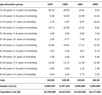
As discussed above, the distribution of the population of Brazil by age and education has been changing rapidly. Table 1 shows the changing distribution of the total male population between ages 15–64 across the 12 age-education groups between 1970 and 2000. This table illustrates the percentage distribution of the male population by particular age-education groups for the whole country in each year. Equation (2) is based on the proportional distribution of the male population in particular age-education groups for each micro-region and year (Xijrt). The crucial facts worth noting are that (1)

there are sharp declines in the share of workers in each age category in the lowest (zero

10_{An approach that allows for the cross-quantity effects that relaxes the restriction on Equation (2), and thus}

(13)

to four years) education cell, and this is especially true among the more recent birth cohorts; and (2) there are general declines in the share of workers in the youngest age group. Within these broad facts, however, it should be emphasized that the increases in educational attainment are not the same among all age groups, and that the declines in the shares of the younger male workforce also differ across education categories. In sum, at least in the aggregate it is clear that there is substantial within-age (education) variation in education (age) in the workforce over our sample period.

Table 1: Male population distributed into particular age-education groups, as percentage shares, Brazil, 1970–2000

Age-education group 1970 1980 1991 2000

15–24 years; 0–4 years of schooling 28.19 20.59 14.61 9.04

15–24 years; 9+ years of schooling 2.74 5.87 5.97 10.24

Total 100.00 100.00 100.00 100.00

Sample size (n) 5,468,939 6,457,351 3,936,080 4,282,888

Population size (N) 25,760,600 32,613,947 43,434,546 53,177,953

(14)

There is a clear increase over time in the proportion of young adults with higher educational attainment (Table 1). At the same time, differences among major regions (North, Northeast, Southeast, South, and Central-West) are pronounced and persistent (data not shown). Higher proportions in the education groups with nine or more years of schooling, especially for men in the 25–34 age group, are observed in the Southeastern, Southern, and Central-Western areas than in the Northern and Northeastern areas. On the other hand, the percentage of adults ages 35–49 with zero to four years of schooling has been decreasing in all regions. There has also been a bigger decline in the proportion of men in low-educated groups in the Southeastern and Southern areas of Brazil than in the Northern and Northeastern areas. Of course, the within-micro-region changes in the relative sizes of age-education cells (not shown, but used to estimate Equation (2)) exhibit much more heterogeneity, both over time and across areas, than the changes for the five major regions of Brazil.

Differences in the timing and speed of the education and fertility transitions led to substantial temporal differences in the education and age distributions across regions, states, and municipalities. Figure 1 illustrates the distribution of men in the highest (nine or more years) education cell for 1970, 1980, 1991, and 2000. In addition to showing the improvement in education, these maps show a large degree of regional variation in educational attainment. While the North and Northeast regions have lower proportions of men with nine or more years of schooling, the Southeast, South, and Central-Western regions have higher proportions of men in this highest education group.

(15)

Figure 1: Distribution of the male working-age population with 9+ years of schooling by micro-region and year, Brazil, 1970–2000

(16)

Figure 2: Mean real monthly earnings in Brazilian reais from the main occupation of the male working-age population by age-education group, Brazil, 2000+

+

Nominal earnings were converted to base 1 in January 2002, taking into account changes in currency and inflation. Source: 2000 Brazilian demographic census.

While differentials in earnings are highly influenced by age and years of schooling (Figure 2), in preliminary analyses (data not shown) these differentials also vary by the number of people in each age-education group. For instance, when the proportion of men aged 35–49 with zero to four years of schooling is small in a micro-region, their earnings are closer to those of men of the same age with more education than they are in micro-regions with high proportions of men in this age-education group. This pattern most likely arises because these men are not competing in the labor market as part of a large group of men of the same age and with the same level of education, which translates into an increase in their earnings relative to other groups. However, when the proportion of men in this age-education group is high in the micro-region, they have a disadvantage in earnings compared with the other groups. The same pattern appears in the other age groups.

These results encouraged us to expand the study of the labor market effects of demographic change and educational advances to include composition. However, the persistent differences in earnings by area and time period suggest that we need to use models that account for specific local and period factors.

(17)

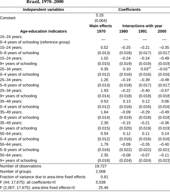
6.2 Estimating the effects of relative group size on earnings

(18)

Table 2: Coefficients and standard errors estimated with the fixed-effects model from Equation (1) for the logarithm of mean real monthly earnings from main occupation+ as the dependent variable, Brazil, 1970–2000

Independent variables Coefficients

Constant 5.33

(0.004)

Main effects Interactions with year

Age-education indicators 1970 1980 1991 2000

15–24 years;

0–4 years of schooling (reference group) –– –– –– –– 15–24 years;

5–8 years of schooling

0.52 (0.013) –0.25 (0.018) –0.21 (0.017) –0.35 (0.017) 15–24 years;

9+ years of schooling

1.02 (0.015) –0.24 (0.019) –0.24 (0.019) –0.49 (0.019) 25–34 years;

0.35 (0.012) 0.10 (0.016) 0.03ns (0.016) –0.01ns (0.016) 25–34 years;

1.26 (0.013) –0.19 (0.018) –0.39 (0.017) –0.48 (0.017) 25–34 years;

1.93 (0.014) –0.22 (0.018) –0.40 (0.018) –0.57 (0.018) 35–49 years;

0.53 (0.012) 0.13 (0.016) 0.12 (0.016) 0.06 (0.016) 35–49 years;

1.64 (0.014) –0.09 (0.019) –0.29 (0.018) –0.49 (0.018) 35–49 years;

2.30 (0.015) –0.15 (0.020) –0.21 (0.019) –0.36 (0.019) 50–64 years;

0.54 (0.012) 0.12 (0.016) 0.11 (0.016) 0.14 (0.016) 50–64 years;

1.79 (0.016) –0.09 (0.022) –0.26 (0.022) –0.40 (0.021) 50–64 years;

2.35 (0.018) –0.08 (0.024) –0.07 (0.024) –0.11 (0.023) Number of observations 19,727

Number of groups 2,008

Fraction of variance due to area-time fixed effects 0.81 F (44; 17,675): all coefficients=0 5,538 F (2,007; 17,675): area-time fixed effects=0 25.46

ns

Non-significant. All other coefficients are significant at least at p<.01. +

Nominal earnings were converted to base 1 in January 2002, taking into account changes in currency and inflation.

Note: Standard errors are reported in parentheses.

(19)

(20)

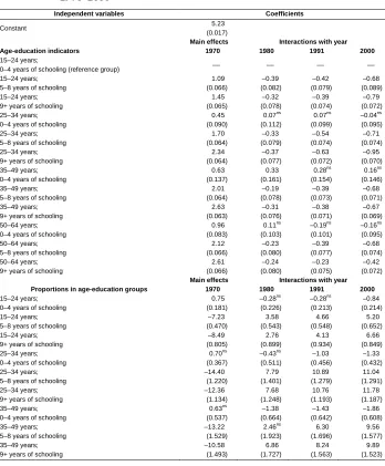
Table 3: Coefficients and standard errors estimated with the fixed-effects model from Equation (2) for the logarithm of mean real monthly earnings from main occupation+ as the dependent variable, Brazil, 1970–2000

Constant 5.23

(0.017)

Age-education indicators 1970 1980 1991 2000

15–24 years;

0–4 years of schooling (reference group) –– –– –– ––

15–24 years; 5–8 years of schooling

1.09 (0.066) –0.39 (0.082) –0.42 (0.079) –0.68 (0.089) 15–24 years;

1.45 (0.065) –0.32 (0.078) –0.39 (0.074) –0.79 (0.072) 25–34 years;

0.45 (0.090) 0.07ns (0.112) 0.07ns (0.099) –0.04ns (0.095) 25–34 years;

1.70 (0.064) –0.33 (0.079) –0.54 (0.074) –0.71 (0.074) 25–34 years;

2.34 (0.064) –0.37 (0.077) –0.63 (0.072) –0.95 (0.070) 35–49 years;

0.63 (0.137) 0.33 (0.161) 0.28ns (0.154) 0.16ns (0.146) 35–49 years;

2.01 (0.064) –0.19 (0.078) –0.39 (0.073) –0.68 (0.071) 35–49 years;

2.63 (0.063) –0.31 (0.076) –0.38 (0.071) –0.67 (0.069) 50–64 years;

0.96 (0.083) 0.11ns (0.103) –0.19ns (0.101) –0.16ns (0.095) 50–64 years;

2.12 (0.066) –0.23 (0.080) –0.39 (0.077) –0.68 (0.074) 50–64 years;

2.61 (0.066) –0.24 (0.080) –0.23 (0.075) –0.42 (0.072)

Proportions in age-education groups 1970 1980 1991 2000

0.75 (0.181) –0.28ns (0.226) –0.28ns (0.213) –0.84 (0.214) 15–24 years;

–7.23 (0.470) 3.58 (0.543) 4.66 (0.548) 5.20 (0.652) 15–24 years;

–8.49 (0.805) 2.76 (0.899) 4.13 (0.934) 6.66 (0.849) 25–34 years;

0.70ns (0.367) –0.43ns (0.511) –1.03 (0.456) –1.33 (0.432) 25–34 years;

–14.40 (1.220) 7.79 (1.401) 10.89 (1.279) 11.04 (1.291) 25–34 years;

–12.36 (1.134) 7.68 (1.248) 10.76 (1.193) 11.78 (1.187) 35–49 years;

0.63ns (0.537) –1.38 (0.664) –1.43 (0.642) –1.86 (0.608) 35–49 years;

–13.22 (1.529) 2.46ns (1.923) 6.30 (1.696) 9.56 (1.577) 35–49 years;

(21)

Table 3: (Continued)

–1.31 (0.434)

–0.83ns

(0.594)

1.05ns

(0.592)

0.27ns

(0.558) 50–64 years;

–23.51 (4.258)

9.60ns

(5.325)

10.25 (5.130)

19.88 (4.526) 50–64 years;

–14.32 (4.592)

11.18 (5.369)

11.91 (4.890)

15.45 (4.681)

Number of observations 19,727

Number of groups 2,008

Fraction of variance due to area-time fixed effects 0.86

F (92; 17,627): all coefficients=0 2,902

F (2,007; 17,627): area-time fixed effects=0 18.80

ns

Non-significant. All other coefficients are significant at least at p<.05. +

Nominal earnings were converted to base 1 in January 2002, taking into account changes in currency and inflation.

Note: Standard errors are reported in parentheses.

Sources: 1970, 1980, 1991, and 2000 Brazilian demographic censuses.

(22)

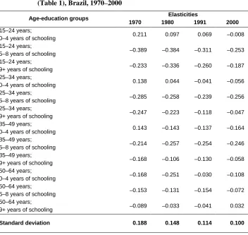
Table 4: Effects of proportion of male working-age population by age-education groups (factor-price elasticities) on mean real monthly earnings from main occupation+ (dependent variable), based on Equation (2) (Table 3), using the national age-education distribution (Table 1), Brazil, 1970–2000

Age-education groups Elasticities

1970 1980 1991 2000

15–24 years;

0–4 years of schooling 0.211 0.097 0.069 –0.008 15–24 years;

5–8 years of schooling –0.389 –0.384 –0.311 –0.253 15–24 years;

9+ years of schooling –0.233 –0.336 –0.260 –0.187 25–34 years;

0–4 years of schooling 0.138 0.044 –0.041 –0.056 25–34 years;

0–4 years of schooling 0.143 –0.143 –0.137 –0.164 35–49 years;

9+ years of schooling –0.089 –0.033 –0.041 0.032

Standard deviation 0.188 0.148 0.114 0.100

+

(23)

Among the least-educated workers for three age groups (15–24 years, 25–34 years, and 35–49 years), the elasticities start out as positive in 1970, but become negative over time. This result means that the greater proportion of men with between zero and four years of schooling (Table 1) generated positive effects on their earnings in previous decades. However, the proportions of the least-educated men have had negative effects on their earnings (Table 4) in recent years, even with lower shares in the population (Table 1). These estimates might suggest that the Brazilian labor market has not needed as many men with low levels of education in recent years as it did in previous decades. This result is especially interesting, and might be explained by the increasing openness of the economy. The exposure to competition from manufactured goods produced using low-skilled and cheap labor could be reducing the demand for the least-educated Brazilians in the labor market. For men ages 50–64 with zero to four years of schooling, elasticities were already negative in 1970, and were moving toward zero in 1991.

Table 4 also shows that the elasticities are more negative among age-education groups with more education (five to eight years of schooling and at least nine years of schooling) in 1970, except for the 50–64 age group. Moreover, as is suggested by the coefficient estimates presented in Table 3, these effects are becoming less negative over time among the groups with higher levels of education. For instance, an increase of 10% in the number of men ages 25–34 with nine or more years of schooling would have reduced their earnings by 2.5% (–0.247) in 1970 and by 0.5% in 2000. We also observe this clear decline in the magnitude (toward zero) of these elasticities over time for men ages 35–49 years with nine or more years of education. For men ages 15–24 years with nine or more years of schooling, there was a decline after 1980. For those ages 50–64 with five to eight years of schooling, elasticities declined in 2000. For men in three age groups with five to eight years of schooling (15–24 years, 25–34 years, and 35–49 years), the impact was strongly negative from 1970 through 2000. As can be seen in Table 4, an increase of 10% in the number of people ages 15 to 24 with five to eight years of schooling would have reduced their earnings by 3.9% (–0.389) in 1970 and 2.5% in 2000. Among young men (ages 25–34) with five to eight years of schooling, the impact on earnings declined from –2.9% in 1970 to –2.6% in 2000. Among experienced adults (ages 35–49) with five to eight years of schooling, the elasticities increased slightly, from –2.1% in 1970 to –2.5% in 2000.

(24)

the elasticities for the groups with zero to four years of education may be indicative of a low demand for labor without either education or experience.

The estimates in Table 4 go beyond the preceding literature by including the age-education cell sizes (proportion of men in each age-age-education group, cohort size, relative supply, labor supply, cell density, or own-quantity effects). The central question in evaluating this exercise is: Would it make a difference if we examined wage changes without accounting for changes in the relative sizes of the age-education cells? In other words, does using a formal labor-demand approach produce better results than could be obtained by just describing changes in the structure of wages using age and education indicators? Equation (1) effectively has wages determined by age-education indicators only, taking into account area-time fixed effects (Table 2). Unsurprisingly, the coefficients on the age-education indicators do not differ greatly from those presented in Table 3.

To answer the central question above, we can compare the relative predictive performances of the estimates from the formal demand model of Equation (2), in Table 3; to those of the estimates of the standard model, which includes all of the area-time fixed effects and time-varying age-education indicators, of Equation (1), in Table 2. Obviously, there are many ways to make this comparison, but we may want to start with the following question: For each year and each age-education cell, what can be gained by our new approach of adding the cell-density (group proportion), which is included in the estimates presented in Table 3? We make this comparison for each year and age-education group by: (a) estimating the absolute prediction errors (predicted earnings minus observed earnings) for each micro-region, year, and age-education group, based on the estimates of Equation (1) (Table 2) and Equation (2) (Table 3); (b) taking the average value across all 502 micro-regions of the absolute prediction errors for each year and age-education group, based on the estimates of Tables 2 and 3; and (c) calculating the ratio of the average absolute deviations of prediction errors from Equation (2) to the average absolute deviations of prediction errors from Equation (1) for each year and age-education group. The 48 ratios (four years and 12 age-education groups) of average absolute deviations of prediction errors from Equation (2) to average absolute deviations from Equation (1) equal one if the two absolute deviations are equal, more than one if Equation (2) performs worse than Equation (1), and below one if Equation (2) is better than the baseline.

Table 5 illustrates the comparisons between predictions of Equations (1) and (2). Most of the ratios are below one unit; the labor-demand model of Equation (2) generally performs better than the atheoretic model of Equation (1). The average ratio across all year-age-education cells is 0.94.11

11_{For 34 of the 48 age-education-year cells, the ratio from Equation (2) to Equation (1) is below unity in}

(25)

Table 5: Ratios of average absolute deviations of prediction errors from Equation (2) to average absolute deviations of prediction errors from Equation (1), Brazil, 1970–2000

Age-education groups Ratios

1970 1980 1991 2000

15–24 years;

0–4 years of schooling 0.985 0.964 0.990 0.982

15–24 years;

9+ years of schooling 0.920 0.860 0.976 0.973

25–34 years;

35–49 years;

50–64 years;

Average 0.915 0.938 0.960 0.960

Sources: 1970, 1980, 1991, and 2000 Brazilian demographic censuses and Tables 2 and 3.

In some senses, this suggests there is a substantial gain to specifying the formal model, as the standard model in Table 2 is itself very heavily specified because it includes area-year fixed effects. Thus, Equation (1) accounts for a substantial amount of the variation in average monthly earnings in this sample. In sum, accounting for area and time differences in changes in age-education group proportions adds substantially to the ability to track changes in relative earnings.12 The comparisons in Table 5 also

assume a quadratic loss function over prediction errors, the improvement looks even greater (this squared average equals 0.90, compared to the absolute average of 0.94).

12_{Using a model that includes all the area-time fixed effects and indicator variables for each age-education}

(26)

demonstrate that, generally, the biggest gain from specifying a labor-demand model lies in the prediction of earnings of the least-educated workers. Except for the 15-24-year-olds, the improvement in predictive power using the labor-demand model is greatest for the group with zero to four years of schooling. The gains to the labor-demand model are generally a bit smaller in 2000 than in 1970. This is a consequence of the relative decline in the effects of population shares on monthly earnings (elasticities moving toward zero over time) that occurred in many age-education cells (Table 4).

6.3 Robustness considerations

Taking into account age and educational composition, in addition to the direct impact of age and education, makes a sizeable difference in the estimation of the earnings profiles of Brazilian workers. But are the elasticities calculated from our models unbiased estimates of the effect of cohort size? Inter-micro-regional migration is perhaps the most important issue, since internal population flows are influenced by the availability of jobs and levels of earnings in the sending and receiving areas. Assuming migrants respond to relative wage differentials, endogenous migration may bias the estimated negative effects on wages toward zero, which implies that our estimates understate the absolute values of the effects13. In addition, the parameter estimates could be biased if, within micro-regions, young people attain more schooling when the returns to education increase as more educated labor becomes relatively scarce. However, like the bias introduced by endogenous migration, endogenous education would also reduce the absolute values of the (negative) estimated parameters. Another potential difficulty might arise from our implicit assumption that the sub-aggregates of male labor are separable in production from those of female labor. We are not sure what the direction of any such bias might be, but preliminary explorations suggest that it is small.14

comparisons, we see that the average ratio from Equation (2) to this reduced model would only be 0.29 (all ratios below unity), and that the squared average would be 0.11.

13_{An exercise was conducted in order to test the influence of internal migration flows in our models. A}

methodological approach was developed by integrating gravitational models (Stillwell 2009) and mathematical equations (Rogers and Castro 1981). The findings follow the initial hypothesis, which stated that, by controlling for migration flows, the negative impact of cohort size on earnings would be even more negative than estimates that did not take into account population flows. Adding migration to the models would then result in even stronger results for the age-education group proportions, meaning that we would understate the importance of our approach in terms of the gains it offers in the ability to track changing wage inequality.

14_{We have the same census information for each micro-region on the age-education structure of the female}

(27)

factor-7. Conclusions

In this study we have tackled an old question, but in a different context and with a different way of extracting lessons from the data. Interesting and important results concerning the effects of shifts in the age distribution of the working-age population have been obtained by a series of authors who looked at this question in the context of the effect of the baby boom generation on the earnings of different cohorts in the U.S. But this issue has received little attention in the countries of Asia and Latin America, which are now experiencing substantial shifts in their age distributions due to large and rapid declines in fertility. In these countries, the shifts in the age distribution have also been accompanied by dramatic increases in educational attainment, which might be expected to alter earnings distributions. A major difference between the U.S. and Latin American countries, such as Brazil, is the magnitude of regional differences in the timing of both the educational and the demographic transitions. These changes were fairly homogeneous across American states, but have varied enormously across different geographical areas in Brazil. This heterogeneity both motivates and enhances the value of our microeconomic geographical approach to the problem.

Our main result is simply that relative group size matters. The proportion of the male population in age-education groups has a negative impact on earnings, mainly for workers with higher levels of education. The potential for biases induced by a number of effects for which we could not adjust means that, if anything, the true effects of changing relative quantities are larger in absolute value than our estimates suggest. The results imply that workers classified by age-education group are not perfect substitutes in the labor market, as a larger cohort-education size generally depresses earnings. Moreover, the effects seem to be more pronounced for workers under age 50 in the middle education group, who have become a much larger part of the workforce in the past 30 years. In addition, while there may have been shifts in relative demand over the 30-year time span we have examined, they do not—unlike in the United States—appear to have been large enough to completely offset the negative effects of variations in cohort size (proportion of men in age-education groups) on earnings. Our confidence in the estimates is heightened by our inclusion of area-time fixed effects, which account

(28)

for any demand shocks specific to a place and time, and put the burden of identification on within-area changes in relative supply over time.

8. Acknowledgments

(29)

References

Autor, D., Katz, L., and Krueger, A. (1998). Computing inequality: Have computers changed the labor market? Quarterly Journal of Economics 113(4): 1169–1214.

doi:10.1162/003355398555874.

Barro, R.J. and Lee, J.W. (2001). International data on educational attainment: Updates

and implications. Oxford Economic Papers 53(3): 541–563.

doi:10.1093/oep/53.3.541.

Berger, M. (1985). The effect of cohort size on earnings growth: A reexamination of the evidence. Journal of Political Economy 93(3): 561–573. doi:10.1086/261315.

Biagi, F. and Lucifora, C. (2008). Demographic and education effects on

unemployment in Europe. Labour Economics 15(5): 1076–1101.

doi:10.1016/j.labeco.2007.09.006.

Bloom, D.E. and Finlay, J.E. (2009). Demographic change and economic growth in Asia. Asian Economic Policy Review 4(1): 45–64.

doi:10.1111/j.1748-3131.2009.01106.x.

Bloom, D.E. and Freeman, R. (1986). The effects of rapid population growth on labor supply and employment in developing countries. Population and Development

Review 12(3): 381–414. doi:10.2307/1973216.

Bloom, D.E., Canning, D., and Fink, G. (2011). Implications of population aging for economic growth. Boston: Harvard Center for Population and Development Studies (Program on the Global Demography of Aging working paper; 64).

doi:10.3386/w16705.

Bloom, D.E., Canning, D., and Malaney, P.N. (2000). Population dynamics and economic growth in Asia. Population and Development Review 26: 257–290.

Bloom, D.E., Canning, D., and Sevilla, J. (2003). The demographic dividend: A new

perspective on the economic consequences of population change. Santa Monica:

RAND.

Bloom, D.E., Canning, D., Fink, G., and Finlay, J.E. (2009). Fertility, female labor force participation, and the demographic dividend. Journal of Economic Growth 14(2): 79–101. doi:10.1007/s10887-009-9039-9.

Bloom, D.E., Freeman, R., and Korenman, S. (1987). The labour-market consequences of generational crowding. European Journal of Population 3(2): 131–176.

(30)

Borjas, G.J. (2003). The labor demand curve is downward sloping: Reexamining the impact of immigration on the labor market. Quarterly Journal of Economics 118(4): 1335–1374. doi:10.1162/003355303322552810.

Borjas, G.J., Freeman, R.B., Katz, L.F., DiNardo, J., and Abowd, J.M. (1997). How do immigration and trade affect labor market outcomes? Brookings Papers on

Economic Activity 1997(1): 1–90. doi:10.2307/2534701.

Brunello, G. (2010). The effects of cohort size on European earnings. Journal of

Population Economics 23(1): 273–290. doi:10.1007/s00148-009-0250-y.

Corseuil, C. and Foguel, M. (2002). Uma sugestão de deflatores para rendas obtidas a partir de algumas pesquisas domiciliares do IBGE. Brasília: Brazilian Institute of Applied Economic Research (“Instituto de Pesquisa Econômica Aplicada” – IPEA working paper; 897).

Easterlin, R.A. (1978). What will 1984 be like? Socioeconomic implications of recent twists in age structure. Demography 15(4): 397–432. doi:10.2307/2061197.

Feng, W. and Mason, A. (2005). Demographic dividend and prospects for economic

development in China. Paper presented at the United Nations Expert Group

Meeting on Social and Economic Implications of Changing Population Age Structures, Mexico City, Mexico, August 31 – September 02 2005.

Freeman, R. (1979). The effect of demographic factors on age-earnings profiles.

Journal of Human Resources 14(3): 289–318. doi:10.2307/145573.

Gindling, T. and Robbins, D. (2001). Patterns and sources of changing wage inequality in Chile and Costa Rica during structural adjustment. World Development 29(4): 725–745. doi:10.1016/S0305-750X(00)00117-0.

Giovannetti, B. and Menezes-Filho, N. (2006). Trade liberalization and the demand for skilled labor in Brazil. Economía 7(1): 1–20. doi:10.1353/eco.2007.0007.

Grant, J. and Hamermesh, D. (1981). Labor market competition among youths, white women and others. Review of Economics and Statistics 63(3): 354–360.

doi:10.2307/1924352.

Hamermesh, D. (1993). Labor demand. Princeton: Princeton University Press.

Katz, L.F. and Autor, D.H. (1999). Changes in the wage structure and earnings inequality. In: Ashenfelter, O. and Card, D. (eds.). Handbook of labor

(31)

Katz, L.F. and Murphy, K.M. (1992). Changes in relative wages, 1963–1987: Supply and demand factors. Quarterly Journal of Economics 107(1): 35–78.

doi:10.2307/2118323.

Kelley, A.C. and Schmidt, R.M. (2001). Economic and demographic change: A synthesis of models, findings, and perspectives. In: Birdsall, N., Kelley, A.C., and Sinding, S.W. (eds.). Population matters: Demographic change, economic

growth, and poverty in the developing world. Oxford: Oxford University Press:

67–105.

Korenman, S. and Neumark, D. (2000). Cohort crowding and youth labor markets: A cross-sectional analysis. In: Blanchflower, D. and Freeman, R. (eds.). Youth

employment and joblessness in advanced countries. Chicago: NBER Chicago

University Press: 57–105.

Lam, D. and Marteleto, L. (2005). Small families and large cohorts: The impact of the demographic transition on schooling in Brazil. In: Lloyd, C.B., Behrman, J.R., Stromquist, N.P., and Cohen, B. (eds.). The changing transitions to adulthood in

developing countries: Selected studies. Washington: The National Academies

Press: 56–83.

Lam, D. and Marteleto, L. (2008). Stages of the demographic transition from a child’s perspective: Family size, cohort size, and children’s resources. Population and

Development Review 34(2): 225–252. doi:10.1111/j.1728-4457.2008.00218.x.

Marcílio, M.L. (2001). Why are Brazil’s public schools so weak? Backwardness in education. Braudel Papers 30: 3–11.

Marcílio, M.L. (2005). História da escola em São Paulo e no Brasil. São Paulo: Imprensa Oficial do Estado.

Mason, A. (2005). Demographic transition and demographic dividends in developed

and developing countries. Paper presented at the United Nations Expert Group

Meeting on Social and Economic Implications of Changing Population Age Structures, Mexico City, Mexico, August 31 – September 02 2005.

Mincer, J. (1974). Schooling, experience, and earnings. New York: National Bureau of Economic Research.

Potter, J.E., Schmertmann, C.P., and Cavenaghi, S.M. (2002). Fertility and

development: Evidence from Brazil. Demography 39(4): 739–761.

(32)

Potter, J.E., Schmertmann, C.P., Assunção, R.M., and Cavenaghi, S.M. (2010). Mapping the timing, pace, and scale of the fertility transition in Brazil.

Population and Development Review 36(2): 283–307.

doi:10.1111/j.1728-4457.2010.00330.x.

Riani, J.L.R. (2005). Determinantes do resultado educacional no Brasil: Família, perfil escolar dos municípios e dividendo demográfico numa abordagem hierárquica e espacial. [Ph.D. Thesis]. Belo Horizonte: Universidade Federal de Minas Gerais (UFMG), Brazilian Center of Development and Regional Planning (“Centro de Desenvolvimento e Planejamento Regional” – CEDEPLAR), Demography Program.

Rios-Neto, E.L.G. and Guimarães, R.R.M. (2010). The demography of education in Brazil: Inequality of educational opportunities based on grade progression probability (1986–2008). Vienna Yearbook of Population Research 8(1): 283– 312. doi:10.1553/populationyearbook2010s283.

Roberts, M. and Skoufias, E. (1997). The long-run demand for skilled and unskilled labor in Colombian manufacturing plants. Review of Economics and Statistics 79(2): 330–334. doi:10.1162/003465397556700.

Rogers, A. and Castro, L.J. (1981). Model migration schedules. Laxenburg: International Institute for Applied Systems Analysis.

Saavedra, J. and Torero, M. (2004). Labor market reforms and their impact over formal labor demand and job market turnover: The case of Peru. In: Heckman, J. and Pagés, C. (eds.). Law and employment: Lessons from Latin America and the

Caribbean. Chicago: University of Chicago Press: 131–182.

Sapozknikov, M. and Triest, R.K. (2007). Population aging, labor demand, and the structure of wages. Boston: Center for Retirement Research at Boston College (CRR working paper; 2007–14).

Shimer, R. (2001). The impact of young workers on the aggregate labor market. The

Quarterly Journal of Economics 116(3): 969–1007.

doi:10.1162/00335530152466287.

Skans, O.N. (2005). Age effects in Swedish local labor markets. Economics Letters 86(3): 419–426. doi:10.1016/j.econlet.2004.09.004.

(33)

Welch, F. (1979). Effects of cohort size on earnings: The baby boom babies’ financial bust. Journal of Political Economy 87(5): S65–S97. doi:10.1086/260823.

(34)