University of New Orleans University of New Orleans
ScholarWorks@UNO
ScholarWorks@UNO
University of New Orleans Theses and
Dissertations Dissertations and Theses
8-5-2010
On Dimensionality Reduction of Data
On Dimensionality Reduction of Data
Harika Rao Vamulapalli University of New Orleans
Follow this and additional works at: https://scholarworks.uno.edu/td
Recommended Citation Recommended Citation
Vamulapalli, Harika Rao, "On Dimensionality Reduction of Data" (2010). University of New Orleans Theses and Dissertations. 1211.
https://scholarworks.uno.edu/td/1211
This Thesis is protected by copyright and/or related rights. It has been brought to you by ScholarWorks@UNO with permission from the rights-holder(s). You are free to use this Thesis in any way that is permitted by the copyright and related rights legislation that applies to your use. For other uses you need to obtain permission from the rights-holder(s) directly, unless additional rights are indicated by a Creative Commons license in the record and/or on the work itself.
On Dimensionality Reduction of Data
A Thesis
Submitted to the Graduate Faculty of the University of New Orleans
in partial fulfillment of the requirements for the degree of
Master of Science in
Engineering
by
Harika Rao Vamulapalli
B.Tech. Jawaharlal Nehru Technological University, 2007
Acknowledgements
I wish to thank those people who contributed to this thesis both directly and indi-rectly. Firstly, I would like to express my gratitude to my supervisor, Dr. Huimin Chen, whose encouragement and support in every aspect to reach the goals, really helped me all the time of my research. I appreciate his patience, guidance and supervision of my work which helped me in the right path. I would like to thank other members in my thesis com-mittee, Dr. X. Rong Li and Dr. Vesselin P. Jilkov, for their support. I would like to thank my labmate, Mr. Gang Liu who have contributed immensely to my personal and professional time. In addition, I wish to dedicate this work to my family and friends who encouraged and supported me during all this time.
Finally, I am grateful to the financial support in part by the research grants from Army Research Office (ARO W911NF-08-1-0409), Louisiana Board of Regents (NSF-2009-PFUND-162), Office of Naval Research (DEPSCoR N00014-09-1-1169) and NASA (EPSCOR DART2).
Table of Contents
List of Figures v
List of Tables vi
Abstract vii
1 Introduction 1
1.1 Motivations & Background . . . 1
1.1.1 Research Objective . . . 2
1.1.2 Organization of Thesis . . . 2
2 Dimensionality Reduction 3 2.1 Introduction . . . 3
2.1.1 Principal Component Analysis . . . 3
2.1.2 Random Projection Methods . . . 4
2.1.3 Fast Johnson-Lindenstrauss Transform . . . 5
2.2 Computational Aspects of Dimensionality Reduction . . . 6
2.3 Connection to Compressed Sensing . . . 7
3 Analysis of Random Projection Algorithms 8 3.1 Error Bound Analysis . . . 8
3.2 Approximate PCA . . . 9
4 Evaluation of Random Projection Algorithms 12 4.1 Motivation . . . 12
4.2 Performance Comparison . . . 12
5 Conclusions and Future Work 17 5.1 Conclusions . . . 17
5.2 Future work . . . 17
Bibliography 18
List of Figures
4.1 Histograms of the pairwise distance ratios,n=50,k=100,= 0.24, Pr(pairwise distance in range)=0.99 . . . 15 4.2 Histograms of the pairwise distance ratios,n=100,k=100,= 0.25, Pr(pairwise
distance in range)=0.99 . . . 16 4.3 Histograms of the pairwise distance ratios,n=200,k=100,= 0.26, Pr(pairwise
distance in range)=0.99 . . . 16
List of Tables
4.1 Finding the appropriate scaling factor using Achlioptas random projection method (n=50) . . . 13 4.2 Finding the appropriate scaling factor using Achlioptas random projection
method (n=100) . . . 13 4.3 Finding the appropriate scaling factor using Achlioptas random projection
Abstract
Random projection method is one of the important tools for the dimensionality re-duction of data which can be made efficient with strong error guarantees. In this thesis, we focus on linear transforms of high dimensional data to the low dimensional space satisfying the Johnson-Lindenstrauss lemma. In addition, we also prove some theoretical results re-lating to the projections that are of interest when applying them in practical applications. We show how the technique can be applied to synthetic data with probabilistic guarantee on the pairwise distance. The connection between dimensionality reduction and compressed sensing is also discussed.
Keywords: principal component analysis, dimensionality reduction, random projec-tion, fast Johnson Lindenstrauss transform
Chapter 1
Introduction
1.1
Motivations & Background
In many machine learning problems, the data available to us can be viewed as distinct objects or items, each of which has a number of attributes. For the sake of clustering or classifying data into different groups, one may model each data entry as a point in certain high-dimensional space. Forn data points, it is convenient to represent the collection of data points by a matrix
A =
u1
u2 ... un
where each data point ui is assumed to have d dimensions.
The problem posed by high-dimensional data is trivial to state, but not so simple to solve. Many algorithms of practical interest such as clustering and classification algorithms can not handle a large number of dimensions efficiently. In addition, a deeper issue called the “curse of dimensionality” has plagued researchers in machine learning and other fields for decades. Generally speaking, for any data entry, as we increase the number of dimensions that it possesses, the complexity involved in processing it for inference purposes increases at an exponential rate. This poses a dilemma: naturally, we want to use as much information as is available to us, on the other hand, as we collect more information, we have to spend dramatically more time trying to make sense of it. Fortunately, there has been abundant research works trying to get around the problems of dealing with data of high-dimensionality. Most of the techniques can be seen as to approximate the high-dimensional data with low-dimensional representations and at the same time to maintain the key structure of the original data to the best extent. We call these techniques a method of dimensionality reduction. Formally, dimensionality reduction involves a mapping from a high-dimensional space to a lower-dimensional one where certain “distance” concept can be preserved.
that the data with reduced dimensions can not be viewed as the compressed version of the original data since data compression concerns to recover the original data from their compressed representations with a distortion below certain desired level. The effectiveness of data compression is usually measured in terms of the number of bits used to represent the data instead of the dimensionality reduction. On the other hand, dimensionality reduction cares about the pairwise distance between two data points rather than the data point itself, which sometimes can be summarized by its distance to the origin.
1.1.1 Research Objective
In machine learning field, the constantly growing data dimension causes severe prob-lems. This difficulty is a problem of long standing and continuing effort. One way is to reduce the dimension: to map the original data in high dimension to another space of low dimension, while preserving important properties as much as possible. There are many ways that map the higher dimensional data to lower dimensional manifold. We would like to focus on methods that map the higher dimensional data into some lower dimensional mani-fold without distorting the pairwise distances. This thesis studies the properties of random projection methods which provide a guarantee of preserving pairwise distances in the lower dimensional space with small distortion. We perform experimental study of two random projection algorithms and compare their performance to the theoretical limit delineated by the Johnson-Lindenstrauss lemma.
1.1.2 Organization of Thesis
The rest of the thesis is organized as follows. Chapter 2 provides background on dimensionality reduction via random projection and its connection to compressed sensing. Chapter 3 contains the analysis of the random projection algorithms. Chapter 4 provides the experimental study of two random projection algorithms based on the synthetic data. Chapter 5 concludes this thesis and indicates possible future directions for high dimensional data analysis.
Chapter 2
Dimensionality Reduction
2.1
Introduction
Dimensionality reduction is a method of obtaining the information from a high di-mensional feature space using fewer intrinsic dimensions. In machine learning, it is very important to reduce high dimensional data set for better classification, regression, presenta-tion and visualizapresenta-tion of data. It is also useful for better understanding of the correlapresenta-tions within the data. This enables us to find the intrinsic dimensionality of the data and provide possibly better generalization capability.
2.1.1 Principal Component Analysis
Principal component analysis (PCA) is perhaps the most popularly used method in dimensionality reduction. Suppose that we want to reduce d-dimensional data to k for n -point data matrix A. Assume that n > d and rank(A) = d, then one possible measure between original data matrix A and its k-dimensional representation B is the Frobenius norm given by
||A||F = X
i X
j
|aij|2
and we want to find the best approximation B∗ such that
B∗ = arg min
rank(B)=k||A−B||F (2.1)
Solution to the above problem boils down to the singular value decomposition (SVD) of A
given by
A=UΛVT
where U and V are orthonormal matrices and D is a diagonal matrix with entries
called the singular values of A. If we take the first k singular values of A and collect the corresponding left and right singular vectors, then we obtain the rank-k approximation ofA
given by
Ak=UkΛkVkT.
It can be shown [8] that B∗ = A
k for any k < d. Note that the PCA minimizes the mean square error between the original data matrix and the rank-k approximation matrix, however, the pairwise distances between the data in the original space and those in their rank approximations can fluctuate arbitrarily. Thus the PCA may find effective low-dimensional features from the original data set but not so meaningful in sketching/hashing high-dimensional data for clustering or classification.
2.1.2 Random Projection Methods
Consider the dimensionality reduction via linear transform so that we can obtain the reduced dimensional data presentation B via
B =AR
whereR is ad×k matrix suitable for preserving the pairwise distance. Note that in Hilbert space, finding such a transform is possible thanks to the following lemma by Johnson and Lindenstrauss [9].
Lemma 1: Suppose that we have ndata points in d-dimensional space. Then ∀ >0, there exists a locally Lipschitz mapping f : Rd → Rk such that ∀k ≥ 12logn
2 and any two rows
u,v∈A, we have
(1−)||f(u)−f(v)||2 ≤ ||u−v||2 ≤(1 +)||f(u)−f(v)||2 (2.2)
Note that the Johnson-Lindenstrauss lemma says that we can preserve the pairwise distance up to a distortion level within (1±) ifk =O(log2n). The original dimensiondof each
data point is irrelevant as far as the pairwise distance is concerned. If we have only two data points, then even if they have hundreds or millions of dimension, the mapping to O(1/2)
dimensional space preserves the distance within (1±). In fact, for any data set A, we can always find a mapping f that preserves the pairwise distance within the desired distortion level. However, for different As, the mapping may not be the same. In fact, the proof in [9] is non-constructive – it shows the existence off but does not say how we actually find one. In practice, there are ways to find a mapping efficiently with high probability satisfying the Johnson-Lindenstrauss lemma. These methods usually rely on random projection of the original high-dimensional data to low-dimensional subspace. By exploiting the concentration property of the pairwise distance, the probability of success can be made arbitrarily large. In fact, the authors in [1] provided an explicit construction of the mapping R summarized by the following lemma.
Lemma 2: Suppose thatA is an n×d data matrix and one needs to reduce the dimension of each data point to k. Let R be a k×d matrix with entries rij given by the following
distribution:
rij =
√
3 with probability1 6
0 with probability23
−√3 with probability16
Let B = 1
√
kAR. For any row u inA, denote by f(u) the corresponding row in B. For any fixed β > 0 and >0, if k > 2/4+22−β3/3 logn, then for any pair of distinct rows u and vin A,
with probability at least (1−n−β), we have (2.2).
Note that the above lemma can be interpreted as “I will preserve all pairwise distances arbitrarily likely in the sense of (2.2) for any given if you allow me to repeatedly generate
R for many times”. This is one of the appealing properties that random projection methods can offer. In fact, if one wants to reduce d-dimensional data points to k-dimensional points with the distortion of pairwise distance to be within (1±), most dimensionality reduction methods such as PCA can not say anything about the lowest dimension k that guarantees the mapping to be within the desired distortion level for arbitrarily chosen n data points.
2.1.3 Fast Johnson-Lindenstrauss Transform
Ailon and Chazelle proposed an efficient algorithm to compute the random projection matrix and the method is called the fast Johnson-Lindenstrauss transform (FJLT) [2]. In particular, the transform is given by
R =P HD (2.3)
where the matrices P and D are random and H is deterministic. The k×d matrix P is sparse. Each entry ofP is either 0 with probability (1−q) or a random number independently drawn from normal distribution with zero mean and variance q−1 with probability q where
q = minnΘp−2logpn d
,1o. The d×d matrix H is a Walsh-Hadamard matrix where d is usually a power of 2. Thed×dmatrixDis a diagonal matrix with thei-th diagonal element
Dii drawn independently from {−1,1}with probability 12.
The computation ofHxcan be evaluated in O(dlogd) operations by an algorithm of fast Fourier transform type [2]. However, computing P HDx requires only O(dlogk). Note that the Walsh-Hadamard matrix has a recursive structure as follows.
H1 = (1 11−1),
Hd= H
d/2 Hd/2
Hd/2 −Hd/2
Letz =Dxand let z1 and z2 be the first and second halves of z. In addition,P1 and P2 are
the left and right halves of P, respectively. We can compute the random projection by
P Hdz = (P1 P2)
H
d/2 Hd/2
Hd/2 −Hd/2
(z1
P1Hd/2(z1+z2) +P2Hd/2(z1−z2)
Assume thatP1 and P2 contain k1 and k2 nonzeros, respectively. Let T(d, k) be the number
of operations required to compute k coefficients out of ad×d Walsh-Hadamard transform. The recurrence relation is given by
T(d, k) = T(d/2, k1) +T(d/2, k2) +d.
In both cases, we haveT(d,0) = 0 andT(d,1) =d. We use induction to show thatT(d, k)≤
2dlog(k + 1). From the above definition, we can see that the computation of the random projection should satisfy
T(d, k) = T(d/2, k1) +T(d/2, k2) +d
≤ dlog(2(k1+ 1)(k2+ 1))
≤ dlog((k1+k2+ 1)2) (for k1+k2 =k ≥1)
≤ 2dlog(k+ 1)
Thus we can see that the fast Johnson-Lindenstrauss transform only takes
T(d, k) =O(dlogk)
shown in [2].
2.2
Computational Aspects of Dimensionality Reduction
In principle, PCA finds the directions of maximal variance from the high-dimensional data and projects the data onto these directions. The runtime of PCA is O(nd2) and it
will be infeasible for problems with very large dimension d. In contrast, random projection methods usually have computational complexity linear in d. In addition, since computing the distance in the original data space takes Ω(d) time while computing the distance in the reduced dimensional space takes Ω(k) time, when k << d, we can infer the distances among data points in the original data space by computing the distances of data points in the reduced dimensional space if the mapping satisfies Johnson-Lindenstrauss lemma. This seems to be an important aspect when one has to cluster high-dimensional data points efficiently.
The construction ofRto satisfy (2.2) with high probability usually relies on random-ized techniques. In [7], the authors used independent and identically distributed Gaussian random variable for rij. Recently, Ailon et al showed that R can be constructed in with sparse Gaussian entries such that the mapping B =AR takes O(k3) runtime [2]. For k not
so small compared to d, the 4-wise independent code matrix was used in [3] to improve the runtime of the mapping to O(dlogk) and [5] showed that the runtime can be made in O(d) with Lean Walsh transform.
2.3
Connection to Compressed Sensing
In compressed sensing, one is interested in sketching d-dimensional signal x by a
k-dimensional measurement y through some encoder Φ such that given
y= Φx
one is able to recover xthrough y by pursuing the maximal sparsity ofx. Note that if xis truly a sparse signal, i.e., most of the elements inxare zero, then one can solve the following constrained optimization problem to recover x.
x∗ = arg max
x ||
x||`0 subject to y= Φx
Since the above problem is NP hard, in practice, one often works on the relaxed version
x∗ = arg max
x ||
x||`1 subject to y= Φx
which can be solved efficiently via linear programming. It turns out that ifxis ak-sparse sig-nal, then there exists a mapping Φ so that with an encoded vectoryof dimensionO(klogd), one can recoverxfromythrough the above sparsity pursuit procedure [6]. Note that finding a good encoder Φ that works for any k-sparse signal x is not easy. Interestingly, it has been shown that a good encoder Φ should satisfy the so called restricted isometry property (RIP) that guarantees ∀x, we have
(1−)||x||2 ≤ ||Φx||2 ≤(1 +)||x||2 (2.4)
Chapter 3
Analysis of Random Projection Algorithms
For dimensionality reduction methods that preserve the pairwise distance with low distortion, Johnson-Lindenstrauss lemma provides theoretical guideline on how well a metric can be embedded from a high dimensional space to a low dimensional one. We know that if the metric is Euclidean, then the embedding can be made with -distortion. For other metrics, it is usually worse: maybe with a constant or logarithmic distortion [11]. In fact, a space with `p-distance metric that satisfies the Johnson-Lindenstrauss lemma is very close being Euclidean: all of its n-dimensional subspaces are isomorphic to Hilbert space with distortion 22O(logn)
[10]. Thus in the subsequent experimental study, we will focus on data points that have been be embedded onto an Euclidean space for performance evaluation with practical settings of d, n, and k.
3.1
Error Bound Analysis
From Lemma 2, it seems that if one needs to reduce the dimensionality of data from
d tok, the lowest reduced dimension would be
k =c 4 + 2β
2/2−3/3logn (3.1)
where c is a positive constant not depending on d. However, it is possible that one may end up with values of n, and β so that k > d, i.e., the bound is meaningless. Thus it is important to know whether there are cases that we can not find any or β to reduce the original dimension through random project method.
Lemma 3: One can not reduce the dimension with arbitrary distortion level in the pairwise distance if and only if the number of data points n grows exponentially in d.
Proof: To fail the dimensionality reduction using Lemma 2, we need
d≥c 4 + 2β
2/2−3/3logn.
For ∈(0,1), we have
2/2−3/3< 1
6 ≤c
4 + 2β d logn.
To ensure that random projection will fail ∀β > 0, we need
logn > d
24c.
Clearly, n has to grow exponentially in d. On the other hand, when n grows exponentially in d, the original Johnson-Lindenstrauss lemma provides a trivial bound, thus the proof is complete.
3.2
Approximate PCA
Random projection can not only preserve the pairwise distance but also preserve the principal directions of the original data matrix with high probability. Let us assume that we want to transform d-dimensional data matrix A tok dimensional matrix B via random projection matrixR given by
B = √1
kAR
where each entry rij in R is drawn independently from standard Gaussian distribution, i.e.,
rij ∼ N(0,1). Assume that d = clog2n where c is some appropriately chosen constant such
that B preserves the pairwise distance within distortion. Now we compute the principal components of B via singular value decomposition such that
B =
k X
i=1
λiaibTi (3.2)
whereλ1 ≥λ2 ≥...≥λk;ai is the left singular vector corresponding to the singular value λi andbiis the right singular vector, respectively. If we only use the best rank-Lapproximation
BL toB, then the PCA algorithm can be made very efficient whenk << d. Let AL be the best rank-L approximation to A and ¯AL be the approximate principal directions obtained via BL, i.e.,
¯
AL=A L X
i=1
bibTi (3.3)
We would expect ¯AL to be a good approximation to AL if the random projection satisfies the Johnson-Lindenstrauss lemma.
Theorem 1: With probability at least 1−4n−(
2
−3)k
4 , the approximation ¯AL satisfies
||A−A¯L||F ≤ ||A−AL||F +||AL||F (3.4)
Proof: Suppose that the SVD yields
A= d X
i=1
B = k X
i=1
λiaibTi
and we have the approximate PCA given by
¯
AL =A L X
i=1
bibTi .
We can see that
||A−A¯L||F = X
i
||Abi−A¯Lbi||2
= X
i
||Abi−A( L X
j=1
bjbTj)bi||2
= ||A||F − k X
i=1
||Abi||2
= ||A−AL||F +||AL||F − k X
i=1
||Abi||2
We want to relate Pk
i=1||Abi||2 to the singular values of B. Note that with probability at
least 1−4n−(
2
−3)k
4 , we have [7]
L X
i=1
λ2i = L X
i=1
||Bbi||2 = L X
i=1
1
k||ARbi||
2
≤ (1 +/2)
L X
i=1
||Abi||2
On the other hand, since vi are the basis for A, with probability at least 1−4n−(
2
−3)k
4 , we
also have
L X
i=1
λ2i ≥
L X
i=1
||Bvi||2 = L X
i=1
1
k||ARvi||
2
≥ (1−/2)
L X
i=1
||Avi||2 = (1−/2)||AL||F
Combining the above inequalities, we can lower boundPk
i=1||Abi||2 by
k X
i=1
||Abi||2 ≥
1−/2
1 +/2||AL||F ≥(1−)||AL||F
Chapter 4
Evaluation of Random Projection Algorithms
4.1
Motivation
We implemented two random projection methods for dimensionality reduction, namely, Achlioptas random projection method [1] and fast Johnson-Lindenstrauss transform (FJLT) [2]. Forndata points of dimensiond, we applied random project algorithms to reduce the di-mension of each data point tok and computed the distances between data points before and after the transform. We are interested in knowing the acceptable k with desired distortion level for some n of practical relevance.
4.2
Performance Comparison
In the experimental study, we generated n data points Xi ∈ Rd (i= 1,2, ..., n) with each element ofXi drawn independently from Gaussian distributionN(0,1). We normalized each data point to have unit distance to the origin. We first implemented Achlioptas random projection algorithm [1] and computed the ratio of pairwise distances before and after the transform. From the histogram of the distance ratio, we chose the distortion tolerancesuch that 99% of the distance ratios fall within the interval [1−,1 +]. In addition, we need to control the sparsity q in implementing the fast Johnson-Lindenstrauss transform. We set
q = logdn. Note that the Johnson-Lindenstrauss lemma states that k = O(log2n) while we
need to find out the scaling factor C such that k = Clog2 n would be meaningful for n and
in some reasonable ranges.
First, we set the number of data points n = 50. We applied Achlioptas random projection method to the input data with varying dimensions dfrom 1024 to 8192. 100 runs for each case were used to determine with different input dimension d and the results are summarized in Table 4.1. We can see that 99% of the ratios between the pairwise distances before and after the dimensionality reduction fall within the distortion level of 0.26 when
k = 100.
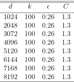
We applied the same procedure for the cases ofn=100 and n=200 with varying input dimension d from 1024 to 8192. The results are listed in Tables 4.2–4.3. Note that does not change significantly as d increases in all cases with fixed n and k. This confirms the theoretical statement of the Johnson-Lindenstrauss lemma. The scaling factor C varies slightly as n increases. Thus to reduce the high dimensional data to low dimension with
Table 4.1: Finding the appropriate scaling factor using Achlioptas random projection method (n=50)
d k C
1024 100 0.24 1.5 2048 100 0.25 1.6 3072 100 0.25 1.6 4096 100 0.25 1.6 5120 100 0.25 1.6 6144 100 0.25 1.6 7168 100 0.26 1.7 8192 100 0.26 1.7
Table 4.2: Finding the appropriate scaling factor using Achlioptas random projection method (n=100)
d k C
1024 100 0.25 1.4 2048 100 0.25 1.4 3072 100 0.25 1.4 4096 100 0.25 1.4 5120 100 0.25 1.4 6144 100 0.25 1.4 7168 100 0.25 1.4 8192 100 0.26 1.5
Table 4.3: Finding the appropriate scaling factor using Achlioptas random projection method (n=200)
d k C
Table 4.4: Finding the acceptable k with various n and d for =0.4
n d k C
50 1024 29 0.4 1.2 50 2048 30 0.4 1.2 50 4096 31 0.4 1.3 100 1024 37 0.4 1.3 100 2048 38 0.4 1.3 100 4096 39 0.4 1.4 200 1024 43 0.4 1.3 200 2048 43 0.4 1.3 200 4096 44 0.4 1.3
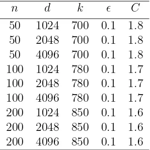
Table 4.5: Finding the acceptable k with various n and d for =0.1
n d k C
50 1024 700 0.1 1.8 50 2048 700 0.1 1.8 50 4096 700 0.1 1.8 100 1024 780 0.1 1.7 100 2048 780 0.1 1.7 100 4096 780 0.1 1.7 200 1024 850 0.1 1.6 200 2048 850 0.1 1.6 200 4096 850 0.1 1.6
tolerable distortion around =0.26, the practical range for k is around 100 for n from 50 to 200. This seems to be still high for the method to be applicable to practical engineering applications.
We also applied fast Johnson-Lindenstrauss transform with multiple runs to find the lowest acceptable dimension k for different scenarios with different values of d, n at the desired distortion level=0.4. Note thatwas chosen based on Achlioptas random projection method with 99% pairwise distances being within the tolerable distortion range. The results are summarized in Table 4.4.
When =0.1, the results are summarized in Table 4.5 with the configurations similar to those in Table 4.4. We can see that the dimension does not reduce significantly when one imposes a more stringent distortion tolerance level.
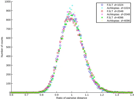
Next, we consider the scenario where the number of data pointsn=50 and the dimen-sion of the output k=100 after applying the Achlioptas random projection method and the fast Johnson-Lindenstrauss transform. We computed the pairwise distances before and after the dimensionality reduction transform and show the ratio of the pairwise distances using histogram in Fig. 4.1. Ideally, we expect the histogram to be centered around 1 with high concentration within 1±. In order to determine the appropriate distortion tolerance level, we set the scaling factor C=1 and computed = qlogCkn. We repeated the same procedure
0.6 0.7 0.8 0.9 1 1.1 1.2 1.3 1.4 0
100 200 300 400 500 600 700 800 900 1000
Ratio of pairwise distance
Number of counts
FJLT d=1024 Achlioptas d=1024 FJLT d=2048 Achlioptas d=2048 FJLT d=4096 Achlioptas d=4096
Figure 4.1: Histograms of the pairwise distance ratios, n=50, k=100, = 0.24, Pr(pairwise distance in range)=0.99
for different scenarios by varying the dimension of each input data point d. From Fig. 4.1, we can see that the results using the fast Johnson-Lindenstrauss transform are similar to those using the Achlioptas random projection method. We found that with probability 0.99, we will preserve the pairwise distance within the distortion no greater than =0.24. This is in line with the results seen in Tables 4.1–4.3.
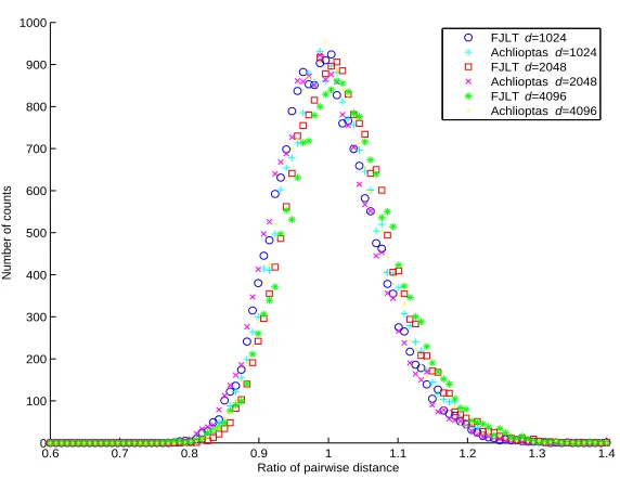
When n=100 and k=100, with varying dimension of each input data point d=1024, 2048 and 4096, the probability of preserving pairwise distance is 0.99 with distortion level
=0.25. We can see from Fig. 4.2 that fast Johnson-Lindenstrauss transform yields similar histograms to those using the Achlioptas random projection method.
Whenn=200 andk=100, the performance comparison between fast Johnson-Lindenstrauss transform and Achlioptas random projection method is shown in Fig. 4.2. We found that with probability 0.99, we will preserve the pairwise distance within the distortion no greater than =0.26.
0.6 0.7 0.8 0.9 1 1.1 1.2 1.3 1.4 0 100 200 300 400 500 600 700 800 900 1000
Ratio of pairwise distance
Number of counts
FJLT d=1024 Achlioptas d=1024 FJLT d=2048 Achlioptas d=2048 FJLT d=4096 Achlioptas d=4096
Figure 4.2: Histograms of the pairwise distance ratios,n=100, k=100,= 0.25, Pr(pairwise distance in range)=0.99
0.6 0.7 0.8 0.9 1 1.1 1.2 1.3 1.4 0 100 200 300 400 500 600 700 800 900 1000
Ratio of pairwise distance
Number of counts
FJLT d=1024 Achlioptas d=1024 FJLT d=2048 Achlioptas d=2048 FJLT d=4096 Achlioptas d=4096
Figure 4.3: Histograms of the pairwise distance ratios,n=200, k=100,= 0.26, Pr(pairwise distance in range)=0.99
Chapter 5
Conclusions and Future Work
5.1
Conclusions
Random projections are a powerful method of dimensionality reduction that provide us with both conceptual simplicity, and very strong error guarantees. The simplicity of pro-jections allows them to be analyzed thoroughly, and this, combined with the error guarantees, makes them a very popular method of dimensionality reduction. In this thesis, we studied two random projection algorithms for dimensionality reduction that preserve the pairwise distances among the data points with small distortion. We found that the fast Johnson-Lindenstrauss transform has comparable performance to the Achlioptas random projection method with better computational efficiency. However, both methods have to sacrifice a small distortion for data points of moderate size.
5.2
Future work
There are many potential areas in which work can be carried out in the future. A brief list is compiled below.
• Lower bound analysis for the reduced dimension k, possibly using Ailon’s method but under special cases, or perhaps a proof of a tight lower bound for specific input data
• An extended study of input distributions and their impact on the distortion of the projection, possibly trying in different ways of defining a distribution (using e.g., the moment generating function of the distribution instead of the mean/variance)
• Using the results derived on input sparsity to derive an analytical solution (or at least to identify some distinct cases) for the distortion as a function of the “true” vector
Bibliography
[1] D. Achlioptas, “Database friendly random projections”, Proc. of ACM Symoisium in
Theory of Computing, New York, NY, USA, pp. 274–281, 2001.
[2] N. Ailon, and B. Chazelle, “Approximate nearest neighbours and the fast Johnson Lindenstrauss transform”, Proc. of ACM Symposium on the Theory of Compututing, Seattle, WA, USA, pp. 557–563, 2006.
[3] N. Ailon and E. Liberty, “Fast dimension reduction using Rademacher series on dual BCH codes”, Symposium on Discrete Algorithms, San Francisco, CA, USA, 2008.
[4] R. Baraniuk, M. Davenport, R. Devore, and M. Wakin, “A simple proof of the restricted isometry property for random matrices”, Contr. Approx., 2008.
[5] K. L. Clarkson, “Tighter bounds for random projection manifolds”,Proc. of 24th Annual
Symposium on Computational Geometry, New York, NY, USA, pp. 39–48, 2008.
[6] D. L. Donoho, “Compressed sensing”, IEEE Trans. on Information Theory, vol. 52, no. 4, pp. 1289–1306, 2006.
[7] S. Dasgupta, and A. Gupta, “An elementary proof of the Johnson-Lindenstrauss lemma”, Technical report 99-006, International Computer science Institute, Berkeley, 1999.
[8] T. Hastie, R. Tibshirani, and J. Friedman, The Elements of Statistical Learning: Data
Mining, Inference and Prediction, Springer, 2001.
[9] W. B. Johnson, and J. Lindenstrauss, “Extensions of Lipschitz mappings into a Hilbert space”, Contemporary Mathematics, 26, pp. 189–206, 1984.
[10] W. B. Johnson, and A. Naor, “The Johnson-Lindenstrauss lemma almost characterizes Hilbert space, but not quite”,Proc. of ACM-SIAM Symposium on Discrete Algorithms, Philadelphia, PA, USA, pp. 885–891, 2009.
[11] J. Matousek, “Bi-Lipschitz embeddings into low dimensional Euclidean spaces”,
Com-ment. Math. Univ. Carolinae, 31, pp. 589–600, 1990.
[12] M. C. Smart, B. V. Ratnakumar, K. B. Chin, L. D. Whitcanack, E. D. Davies, S. Surampudi, M. A. Manzo, P. J. Dalton, “Lithium-ion cell technology demonstration for future NASA applications”, Intersociety Energy Conversion Engineering Conference
(IECEC), Washington, DC, USA, pp. 297–304, 2002.