Relationship between Environmental Quality and Economic Growth in Developing Countries (based on Environmental Performance Index)

Relationship between Environmental Quality and Economic

Growth in Developing Countries (based on Environmental

Performance Index)

Hossein-Ali Fakher, Zahra Abedi*

Department of Environmental Economics, Science and Research branch, Islamic Azad University, Tehran, Iran

Received: 12 February 2017 /Accepted: 2 July 2017

Abstract

In order to evaluate the development levels of countries, economic growth along with environmental quality account for important indices nowadays. The impacts of environmental quality (based on environmental performance index), the direct foreign investment, and trade openness on economic growth in selected developing countries have been scrutinized in the present study. In the present study the Auto Regressive Distributed Lag Model and ARDL bounds test methods were adopted in panel data pertaining to the data of 1983 to 2013 time span. According to the results, a co-integration was found among the model-based variables if economic growth was determined as the dependent variable. The trade openness showed a significant long-run relationship based on the estimated coefficients. Results indicate a positive and significant impact of environmental performance index on economic growth. Moreover, the variable foreign direct investment revealed a positive and significant confirmation. Considering the diagnostic tests findings at 5% level, such problems as serial correlation, functional form, model misspecification, and heteroscedasticity are not present in the estimated model.

Keywords: Economic Growth, Environmental Performance Index, Trade Openness, Foreign Direct Investment

Introduction

There are unclear relationships among foreign direct investment, environmental quality, and economic growth, which appear to have entirely dissimilar patterns in developing countries, for which an essential question is how to maintain the growth process. Environmental restrictions, however, can likely result in reduced regional growth needed for demographic flourish followed by increased unemployment levels. From a different viewpoint, improved developments in growth and sustainability resulting from technological transfer may provide new opportunities and advantages. This issue raises a highly important question in this context, that is, the nature and the extent to which the economic growth and environmental quality are currently interrelated in developing countries. Extensive research has long concentrated on interrelations among foreign direct investment, CO2 emissions, and economic

growth at different countries. The relevant earlier studies can generally be classified into two lines, though; most of practical proofs will continue to be debatable and obscure. The credibility of Environmental Kuznets Curve (EKC) hypothesis is the first to be addressed, in which an inverted-U curve is premised to fit the relationship between economic growth and the environment (Omri et al. 2015). This means that the development of a country exacerbates environmental degradation levels, but it lessens up on attaining a certain level of average revenue. The hypothesis, without any policy interference, is a key to forth coming environmental problems as it predicts economic growth. Grossman and Krueger (1991) initially recommended and confirmed the hypothesis. Later on, it was extensively revised through various data sets and econometric approaches applied by huge research efforts. Contrarily, it was later announced that increased levels of CO2 emissions are not essentially

granted by elevated amounts of domestic income (Friedl and Getzner, 2003; Managi and Jena, 2008). Most recently, a conclusion was drawn by Omri et al. (2014) stating that CO2

emissions have a unidirectional and positive interconnection with economic growth, which extends from CO2 emissions to GDP per capita. Likewise, Omri (2013) suggested a two-way

causality between economic growth and CO2 emissions. Holtz-Eakin et al. (2003), on the

other hand, discovered a monotonic ascending curve; Christopher and Douglason (2011) showed while an N-shaped curve. The economic growth and environmental pollutants are, however, not significantly related as noted by Richmond and Kaufmann (2006), and Rawshan, Kazi, Sharifah, Syed and Mokhtar (2014). An association between foreign direct investment and CO2 emissions is the emphasis of second pattern. There are very scarce

published data on the connection between foreign direct investment and CO2 emissions. Such

a relationship has been pointed out in the literature. For instance, foreign direct investment has been described to be a significant factor affecting pollutants (Acharyya, 2009; Zhang, 2011; Lau Chong and Eng, 2014).

The paper continues with the following structure. Both hypothetical and realistic literature review have been presented in Section 2. The data used are defined in Section 3, and a practical analysis of the findings as well as the technique estimates are given in Section 4. A conclusion is provided in Section 5.

A theoretical and empirical literature review

A literature review is presented here in three subsets: 1) Environmental quality and economic growth, 2) Foreign direct investment and economic growth, and 3) Trade openness and economic growth. The subsets are discussed below, respectively.

Environmental quality and economic growth

There is an instinctive attraction behind the rationality of EKC relation. An increase in material output with a high prioritization at the initial phase of industrialization leads to a swift progression of pollution, which raises more interests in people towards jobs and income compared to unpolluted air and water (Dasgupta et al. 2002). An unavoidable increased consumption of natural resources and pollutant emissions resulting from the fast pollution growth can in turn intensify environmental burden. Rising incomes at the subsequent phase of industrialization will result in more value for the environment by people, enhanced effectiveness in governing foundations, and reduced pollution levels. As a result, a distinct relationship is postulated between economic activity levels and environmental pressure in EKC hypothesis (Grossman and Krueger, 1991; Shafik, 1994; Aldy, 2005; Song et al. 2008; Iwata et al. 2009).

Foreign direct investment and economic growth

Economic growth may be affected both directly and indirectly by foreign direct investment. Foreign investment directly influences increases in production, employment, added value, and export, which in turn directly raise GDP. The individual’s income, for example, is raised by employment and the elevated revenue is directly estimated in GDP. The added value and export have similar processes. GDP, on the other hand, will rise indirectly as a result of foreign investment, including technology transfer, licensed knowledge and techniques, simulation, and job training. Factors that indirectly increase GDP in economic growth include externalities, technology spillover, human capital formation, efficiency, and productivity (Chakraborty, 2001; Borensztein and Lee, 1998). It is expected that products to be delivered with improved quality and lesser costs as a result of improvements in domestic production technology, leading to increased national production and per capita output. To put it differently, the spillover to domestic enterprises renders technology to be a promising basis for productivity benefits. The difference in human capital at various countries has been demonstrated to have an impact on technology capture, ultimately affecting economic growth (Borensztein et al. 1998). The neoclassical economics believes that the only GDP per capita, and not economic growth, is influenced by foreign direct investment, implying that economic growth is not a long-term promoter of foreign direct investment. The modern theory of economic growth, however, deduces that both per capita production and economic growth are under the influence of foreign direct investment (De Mello, 1997).

According to a number of theories, economic growth results from foreign direct investment via such determinants as technology conveyance and spillover as well as productivity elevation, though, contrasting viewpoints have been raised by other theories. Foreign direct investment is predicted by subsequent theories to be damaging to resource apportionment when an established trade is present and price and other finances are disturbed leading to decreased economic growth (Boyd and Smith, 1992). Developing countries often exhibit such a status, where the major problem to be probably a fragile economic configuration such as in appropriate infrastructures, faint human capital, outdated and obsolete technology, etc. Such a structure cannot furnish the means necessary to capture cutting-edge know-how and sciences.

Trade openness and economic growth

whereas better investment exists and goods are produced more abundantly. This would result in rises in the sector’s productivity and export leading to improvement of the economic growth. Other economists (Krueger, 1978; Bhagwati, 1978) further expanded the theory and discussed that trade openness stimulates sectors to specialize where the economic magnitude reaches to the extent that it promotes long-term efficiency and productivity. The international dissemination of progressive technologies has led to defining a positive relationship between trade liberalization and economic growth by new internal growth models (Coe and Helpman, 1995; Grossman and Helpman, 1991a; Romer, 1994). An increased ability is expected for a country having more trade openness in the use of technologies created by modern economies rendering them a faster growth as opposed to a country with low-level trade liberalization. Moreover, the simulation cost is important in the relationship between trade and growth (Edwards, 1998). When poorer countries spend lower costs for simulating innovations in comparison with those in developed economies, the former will flourish faster than the latter followed by an inclination to convergence. According to the above statements, it can be concluded that trading with global industrial countries by developing economies would result in a large achievement. Contrarily, it has been stated that economic growth may be impaired by trade openness. Almeida and Fernandes (2008) believe that such a condition occurs when sectors in a country focus on where core research and development activities are absent. It is also important to note that the goods component of trade composition can have an effect on the growth (Haussmann et al. 2007). The facilitation of directing and accommodating foreign technologies to the indigenous environment is also a factor determining international trade-borne benefits to a country (Grossman and Helpman, 1991).

Theoretical-empirical concept of environmental performance index

Environmental performance index is a very important and composite index, which specifies objectives in order to reach environmental efficiency, measures present situation of each component parts of this index and evaluates how to achieve the desired goals. Environmental performance index emphasizes on two principal objectives of environment protection, including effect of decrease of the bioenvironmental pressures on the humans’ health, promotion of situation of habitats and correct management of natural resources. Quantity of environmental performance index is in a range from 0 to 100 which 100 corresponds with objective and 0 is the worst state.

Materials and methods

Data and description of variable

Yearbook volumes were the sources of data representing labor and FDI. The Yale University (Yale Center for Environmental Law and Policy) and Columbia University (Center for International Earth Science Information Network) in association with the World Economic Forum and the Joint Research Centre of the European Commission have developed EPI. The other variables were obtained from WDI.

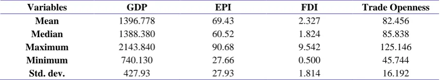
Table 1 shows the statistical summary of all variables. As can be seen, all the variables are presented in logarithmic form in this study.

Table 1. A summary of the variables’ statistics

Variables GDP EPI FDI Trade Openness

Mean 1396.778 69.43 2.327 82.456

Median 1388.380 60.52 1.824 85.838

Maximum 2143.840 90.68 9.542 125.146

Minimum 740.130 27.66 0.500 45.744

Std. dev. 427.93 27.93 1.814 16.192

Source: research findings

Unit roots tests

In order to analyze the co-integration of ARDL bounds tests, the stationary properties has to be first examined followed by determining the integration variables’ arrangement. For this purpose, two panel unit root tests were used developed by Levin et al. (2002) and Im et al. (2003). The tests contain the null hypothesis that a unit root is present in the panel. It, however, was presumed that the unit root process to be commonly shared by the cross-sectional units (Levin et al. 2002). Another assumption, on the other hand, is that unit root process to be individually present in the cross-sectional units (Im et al. 2003). Levin et al. (2002) presented the following panel model for the unit root analysis (Nazlioglu and Soytas, 2012):

∆y_it= 𝜇_𝑖+ 𝜌𝑦_𝑖𝑡−1+ ∑ 𝛼_𝑗∆𝑦_{𝑖𝑡−𝑗}+ 𝛿_𝑖𝑡+ 𝜃_𝑡+ 𝜀_𝑖𝑡

𝑘

𝑗=1

(1)

Where, Δ denotes the first difference operator, 𝜇_𝑖 is the unit specific fixed effects, 𝜃_𝑡 indicates the time effects, and 𝑘 shows the lag length. The null hypothesis 𝜌 = 0 is tested for the whole 𝑖. A rejected null hypothesis implies the presence of a panel stationary process. The developed unit root test (Levin et al. 2002) has a disadvantage of lessening explanatory power when there is a trend in the series. Because of this, the analysis of Levin et al. (2002) is complemented by the test of Im et al. (2003), according to which the unit root test is determined by:

∆y_it= 𝜇_𝑖+ 𝜌𝑦_𝑖𝑡−1+ ∑ 𝛼_𝑗∆𝑦_{𝑖𝑡−𝑗}+ 𝛿_𝑖𝑡+ 𝜃_𝑡+ 𝜀_𝑖𝑡

𝑘

𝑗=1

(2)

For the above equation, 𝐻₀ is defined as unit root to be present in all the country series 𝜌₁ = 𝜌₂ = ⋯ = 𝜌_𝑖 = 0 . The alternate hypothesis is that unit root exists at some countries in the panel data (𝜌_𝑖 < 0 for some 𝑖). Table 2 represents the results of unit root test for the variables.

Based on the data presented in Table 2, the existence of co-integration between data was tested in the next step.

Table 2. Results of panel unit root tests

Variable

LLC test IPS test

Level First difference Level First difference

T-Statistics p-value T-Statistics p-value T-Statistics p-value T-Statistics p-value

𝐥𝐧(𝐘) 3.0891(0) 1.0000 -9.6695(0)*** _{0.0000 1.9175(2) 0.9528 -5.1223(0)}*** _0.0000

𝐥𝐧(𝐄𝐏𝐈) -7.3441 (0)*** _{0.0000 -10.2021 (0)}*** _{0.0000 -5.6128 (0)}** _{0.0000 -4.3082 (0)}** _0.0000

𝐥𝐧(𝐅) -3.0302 (0)*** _{0.0013 -10.2883 (0)}*** _{0.0000 -2.5687(0)}*** _{0.0021 -2.8650(1)}*** _0.0000

𝐥𝐧(𝐓) -3.2836 (0)*** _{0.0005 -9.3726 (0)}** _{0.0000 -2.1805(0)}** _{0.0280 -2.3882(1)}** _0.0049

Notes: Restricted intercept and trend for all variables were applied in all panel unit root tests. The small brackets show the lag length of variables. *, **, and *** indicate the significance at 1%, 5%, and 10% levels, respectively.

ARDL bounds tests for co-integration

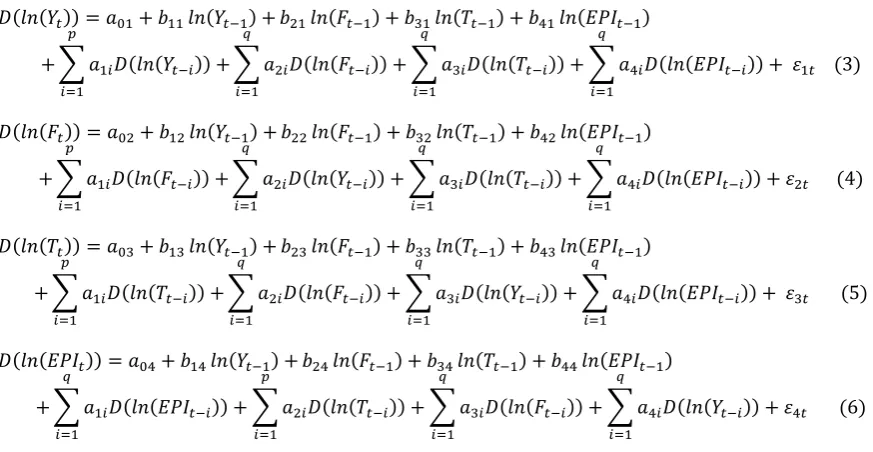
The autoregressive distributed lag (ARDL) co-integration approach was used as a general vector autoregressive (VAR) model of order 𝑝 in 𝑍_𝑡, where 𝑍_𝑡, shows a column vector containing four variables: 𝑍_𝑡 = (𝑌_𝑡𝐹_𝑡𝑇_𝑡𝐸𝑃𝐼_𝑡). The rationale was to practically scrutinize both long-and short-term relationships and dynamic interactions among the desired variables (Environmental Performance Index, Trade Openness, Foreign Direct Investment, and economic growth). Pesaran and Shin (1999) and Pesaran et al. (2001) have developed the ARDL integration method, which, compared to other preceding and outdated co-integration approaches, has three advantages. Firstly, there is no need in ARDL to integrate all the study variables of the same order, which is used when the goal is to integrate elemental variables of order one, order zero or those that are marginally integrated. Secondly, the ARDL test is advantageous as it has a moderately more efficiency regarding sample data with a meager and limited extent. As reported by Harris and Sollis (2003), the third advantage of ARDL technique is that it can be employed to impartially estimate the model in long term. The following is the ARDL model applied in the present research:

𝐷(𝑙𝑛(𝑌𝑡)) = 𝑎01+ 𝑏11𝑙𝑛(𝑌𝑡−1) + 𝑏21𝑙𝑛(𝐹𝑡−1) + 𝑏31𝑙𝑛(𝑇𝑡−1) + 𝑏41𝑙𝑛(𝐸𝑃𝐼𝑡−1)

+ ∑ 𝑎1𝑖𝐷(𝑙𝑛(𝑌𝑡−𝑖)) +

𝑝

𝑖=1

∑ 𝑎2𝑖𝐷(𝑙𝑛(𝐹𝑡−𝑖))

𝑞

𝑖=1

+ ∑ 𝑎3𝑖𝐷(𝑙𝑛(𝑇𝑡−𝑖))

𝑞

𝑖=1

+ ∑ 𝑎4𝑖𝐷(𝑙𝑛(𝐸𝑃𝐼𝑡−𝑖))

𝑞

𝑖=1

+ 𝜀1𝑡 (3)

𝐷(𝑙𝑛(𝐹_𝑡)) = 𝑎02+ 𝑏12𝑙𝑛(𝑌𝑡−1) + 𝑏22𝑙𝑛(𝐹𝑡−1) + 𝑏32𝑙𝑛(𝑇𝑡−1) + 𝑏42𝑙𝑛(𝐸𝑃𝐼𝑡−1)

+ ∑ 𝑎_1𝑖𝐷(𝑙𝑛(𝐹_𝑡−𝑖)) +

𝑝

𝑖=1

∑ 𝑎_2𝑖𝐷(𝑙𝑛(𝑌_𝑡−𝑖))

𝑞

𝑖=1

+ ∑ 𝑎_3𝑖𝐷(𝑙𝑛(𝑇_𝑡−𝑖))

𝑞

𝑖=1

+ ∑ 𝑎_4𝑖𝐷(𝑙𝑛(𝐸𝑃𝐼_𝑡−𝑖))

𝑞

𝑖=1

+ 𝜀_2𝑡 (4)

𝐷(𝑙𝑛(𝑇_𝑡)) = 𝑎₀₃+ 𝑏₁₃𝑙𝑛(𝑌_𝑡−1) + 𝑏₂₃𝑙𝑛(𝐹_𝑡−1) + 𝑏₃₃𝑙𝑛(𝑇_𝑡−1) + 𝑏₄₃𝑙𝑛(𝐸𝑃𝐼_𝑡−1)

+ ∑ 𝑎_1𝑖𝐷(𝑙𝑛(𝑇_𝑡−𝑖)) +

𝑝

𝑖=1

∑ 𝑎_2𝑖𝐷(𝑙𝑛(𝐹_𝑡−𝑖))

𝑞

𝑖=1

+ ∑ 𝑎_3𝑖𝐷(𝑙𝑛(𝑌_𝑡−𝑖))

𝑞

𝑖=1

+ ∑ 𝑎_4𝑖𝐷(𝑙𝑛(𝐸𝑃𝐼_𝑡−𝑖))

𝑞

𝑖=1

+ 𝜀_3𝑡 (5)

𝐷(𝑙𝑛(𝐸𝑃𝐼𝑡)) = 𝑎04+ 𝑏14𝑙𝑛(𝑌𝑡−1) + 𝑏24𝑙𝑛(𝐹𝑡−1) + 𝑏34𝑙𝑛(𝑇𝑡−1) + 𝑏44𝑙𝑛(𝐸𝑃𝐼𝑡−1)

+ ∑ 𝑎1𝑖𝐷(𝑙𝑛(𝐸𝑃𝐼𝑡−𝑖))

𝑞

𝑖=1

+ ∑ 𝑎2𝑖𝐷(𝑙𝑛(𝑇𝑡−𝑖))

𝑝

𝑖=1

+ ∑ 𝑎3𝑖𝐷(𝑙𝑛(𝐹𝑡−𝑖))

𝑞

𝑖=1

+ ∑ 𝑎4𝑖𝐷(𝑙𝑛(𝑌𝑡−𝑖))

𝑞

𝑖=1

All variables in the above equations are as already described in Section 4, 𝑙𝑛(0) denotes the logarithm operator, 𝐷 marks the first difference, and 𝜀_𝑡 indicates the error terms.

The joint F-statistic mainly underlies the bounds test. When the null hypothesis is the absence of a co-integration, the asymptotic distribution of the joint F-statistic will not be standardized. Estimation of equations ((3)–(6)) by ordinary least squares (OLS) is the initial stage in the ARDL bounds method.

The four equations tests are estimated to test relationships among the variables in long-term through running an F-test to delong-termine the joint significance of the coefficients for the variables’ lagged levels, that is: 𝐻0: 𝑏1𝑖 = 𝑏2𝑖 = 𝑏3𝑖 = 𝑏4𝑖 = 0 against the alternative one: H₁: b_1i≠ b_2i≠ b_3i≠ b_4i ≠ 0 for 𝑖 = 1, 2, 3, 4. Pesaran et al. (2001) determined two sets of critical values for a certain significance level. Calculation of the first level assumes that ARDL model integrates all variables of order zero.

Estimation of the second level, however, is based on the postulation that the model integrates variables of order one. A higher value of the test statistic than the upper critical bounds value will reject 𝐻0 concerning the lack of co-integration, though, an F-statistic lower

than bounds value will not refuse 𝐻₀. The co-integration test will, however, be unconvincing under other conditions.

The Akaike information criteria were used to choose an uppermost lag order of 2 for the provisional ARDL vector error correction model. The estimated F-statistics (Table 3) represent the ARDL-OLS regressions assuming each variable as a dependent (normalized) one. The values include: for Eq. (1), 𝐹𝑌 (𝑌\𝐹, 𝑇, 𝐸𝑃𝐼) = 3.365; for Eq. (2), 𝐹𝑇 (𝑇\ 𝑌, 𝐹, 𝐸𝑃𝐼) = 3.736; for Eq. (3), 𝐹_𝐸𝑃𝐼 (𝐸𝑃𝐼\𝑌, 𝐹, 𝑇) = 1.368 and for Eq. (4), 𝐹_𝐹 (𝐹\ 𝑌, 𝑇, 𝐸𝑃𝐼) = 6.542.

Based on the above findings, if economic growth is the dependent variable, a clear drawn-out association exists between the variables as the estimated F-statistic (6.542) exceeds the upper-bound critical value (4.15) at a level of 5%. This, as a result, rejects that the lack of co-integration (𝐻₀) among the variables (Eq. 6). Nonetheless, the 𝐻₀ regarding the absence of co-integration is not rejected for equations (3)–(5).

Granger short-run and long-run causality tests

Following the establishment of co-integration, the long-run model of conditional ARDL (p,𝑞₁, 𝑞₂, 𝑞₃, 𝑞₄) is calculated for ln(F_t) as follows:

ln(𝐹_𝑡) = 𝑎0+ ∑ 𝑎1𝑖ln(𝐹𝑡−𝑖)

𝑝

𝑖=1

+ ∑ 𝑎_2𝑖ln(𝑌_𝑡−𝑖)

𝑞2

𝑖=0

+ ∑ 𝑎_3𝑖ln(𝑇_𝑡−𝑖)

𝑞3

𝑖=0

+ ∑ 𝑎_4𝑖ln(𝐸𝑃𝐼_𝑡−𝑖)

𝑞4

𝑖=0

+ 𝜀_𝑡 (7)

Table 3. Bounds test results

Dependent Variable AIC lags F-statistic Decision

𝐅_𝐅(𝐅\𝐘, 𝐓, 𝐄𝐏𝐈) 2 6.542 Co-integration

𝐅_𝐘(𝐘\ 𝐅, 𝐓, 𝐄𝐏𝐈) 2 3.365 No co-integration

𝐅_𝐓(𝐓\𝐘, 𝐅, 𝐄𝐏𝐈) 1 3.736 No co-integration

𝐅_𝐄𝐏𝐈(𝐄𝐏𝐈\𝐘, 𝐅, 𝐓) 2 1.368 No co-integration

Lower-bound critical value at 1% 3.08

Upper-bound critical value at 1% 4.21

Table 4. Results of long-run model calculation

Dependent variable: Economic growth

Variables Coefficient Probability

𝐂 -1.32 0.15

𝐥𝐧(𝐄𝐏𝐈) 1.51 0.01

𝐥𝐧(𝐅𝐃𝐈) 0.43 0.01

𝐥𝐧(𝐓) 0.051 0.001

𝐅 − 𝐬𝐭𝐚𝐭𝐢𝐬𝐭𝐢𝐜 8.67 0.0001

𝐑 − 𝐬𝐪𝐮𝐚𝐫𝐞𝐝 0.73

𝐃𝐖 − 𝐬𝐭𝐚𝐭𝐢𝐬𝐭𝐢𝐜 1.82

Source: Research findings

All the above variables have previously been defined. Using AIC. Eq. 6, the orders (𝑝, 𝑞₁, 𝑞₂, 𝑞₃, 𝑞₄) of ARDL model in the four variables are selected and estimated via the following ARDL (1, 0, 0, 0, 0, 0) specification. Table 4 indicates the results of long-run GDP normalization.

The calculated long-run relationship coefficients are significant for trade liberalization (Table 4). There is a positive significant impact (at a level of 5%) by environmental performance index on economic growth. Moreover, the variable foreign direct investment received a positive and significant confirmation.

An error correction model together with the long-run estimates was calculated to obtain the short-run dynamic parameters according to Odhiambo (2009) and Narayan and Smyth (2008). The presence of Granger-causality in at least one direction was reflected by the long-run association between the variables specified by the F-statistic and the lagged error-correction term. The F-statistic on the descriptive variables denotes a short-run causal impact.

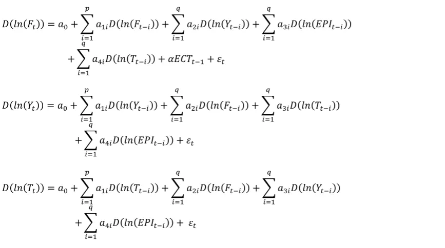
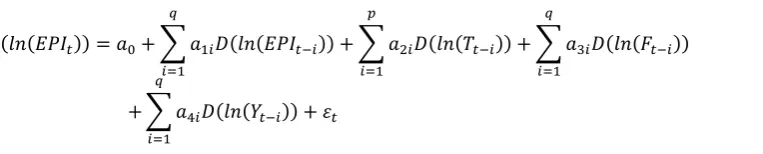
The long-run causal relationship, however, is determined by the t-statistic for the coefficient of the lagged error-correction term (Odhiambo, 2009; Narayan and Smyth, 2006). An error-correction term is used (Narayan and Smyth, 2006; Morley, 2006) to estimate the equation, which rejects a lack of co-integration (𝐻₀). The following equations define vector error correction model:

𝐷(𝑙𝑛(𝐹𝑡)) = 𝑎0+ ∑ 𝑎1𝑖𝐷(𝑙𝑛(𝐹𝑡−𝑖))

𝑝

𝑖=1

+ ∑ 𝑎2𝑖𝐷(𝑙𝑛(𝑌𝑡−𝑖))

𝑞

𝑖=1

+ ∑ 𝑎3𝑖𝐷(𝑙𝑛(𝐸𝑃𝐼𝑡−𝑖))

𝑞

𝑖=1

+ ∑ 𝑎4𝑖𝐷(𝑙𝑛(𝑇𝑡−𝑖))

𝑞

𝑖=1

+ 𝛼𝐸𝐶𝑇𝑡−1+ 𝜀𝑡 (8)

𝐷(𝑙𝑛(𝑌𝑡)) = 𝑎0+ ∑ 𝑎1𝑖𝐷(𝑙𝑛(𝑌𝑡−𝑖))

𝑝

𝑖=1

+ ∑ 𝑎2𝑖𝐷(𝑙𝑛(𝐹𝑡−𝑖))

𝑞

𝑖=1

+ ∑ 𝑎3𝑖𝐷(𝑙𝑛(𝑇𝑡−𝑖))

𝑞

𝑖=1

+ ∑ 𝑎4𝑖𝐷(𝑙𝑛(𝐸𝑃𝐼𝑡−𝑖))

𝑞

𝑖=1

+ 𝜀𝑡 (9)

𝐷(𝑙𝑛(𝑇𝑡)) = 𝑎0+ ∑ 𝑎1𝑖𝐷(𝑙𝑛(𝑇𝑡−𝑖))

𝑝

𝑖=1

+ ∑ 𝑎2𝑖𝐷(𝑙𝑛(𝐹𝑡−𝑖))

𝑞

𝑖=1

+ ∑ 𝑎3𝑖𝐷(𝑙𝑛(𝑌𝑡−𝑖))

𝑞

𝑖=1

+ ∑ 𝑎_4𝑖𝐷(𝑙𝑛(𝐸𝑃𝐼_𝑡−𝑖))

𝑞

𝑖=1

𝐷(𝑙𝑛(𝐸𝑃𝐼_𝑡)) = 𝑎0+ ∑ 𝑎1𝑖𝐷(𝑙𝑛(𝐸𝑃𝐼𝑡−𝑖)) 𝑞

𝑖=1

+ ∑ 𝑎_2𝑖𝐷(𝑙𝑛(𝑇_𝑡−𝑖))

𝑝

𝑖=1

+ ∑ 𝑎_3𝑖𝐷(𝑙𝑛(𝐹_𝑡−𝑖))

𝑞

𝑖=1

+ ∑ 𝑎_4𝑖𝐷(𝑙𝑛(𝑌_𝑡−𝑖))

𝑞

𝑖=1

+ 𝜀_𝑡 (11)

The short-run dynamic coefficients of the model’s convergence to equilibrium are indicated by 𝑎1𝑖, 𝑎2𝑖, 𝑎3𝑖 and 𝑎4𝑖 in the above equations, and 𝑎 denotes the adjustment speed.

OLS regression separately estimates Equations (8)–(11). Table 5 reveals the results of the short-run dynamic coefficients alongside the long-run relationships estimated by Eq. (8). A highly fitting regression was obtained for the basic ARDL Eq. (8) with a total significance level of 1% for the model.

All diagnostic tests against serial correlation (Durbin Watson test and Breusch– Godfrey test), heteroskedasticity (White heteroskedasticity test), and normality of errors (Jarque–Bera test) also approve the model. According the Ramsey RESET test, the model is properly defined as well. Table 6 shows the entire results of all the tests.

The short-run dynamics were used to test the long-run coefficient stability, followed by the estimation of the ECM model given by Eq. (7). In addition, the diagnostic tests are reported in Table 6.

Table 5. Results of short-run model assessment

Dependent variable: Economic growth

Variables Coefficient Probability

𝐂 -0.05 0.19

𝐃(𝐥𝐧(𝐄𝐏𝐈)) 1.60 0.01

𝐃(𝐥𝐧(𝐅𝐃𝐈)) - 0.14 0.36

𝐃(𝐥𝐧(𝐓)) 0.021 0.002

𝐄𝐂𝐓(−𝟏) -0.76 0.0003

𝐅 − 𝐬𝐭𝐚𝐭𝐢𝐬𝐭𝐢𝐜 4.87 0.001

𝐑 − 𝐬𝐪𝐮𝐚𝐫𝐞𝐝 0.68

𝐃𝐖 − 𝐬𝐭𝐚𝐭𝐢𝐬𝐭𝐢𝐜 1.96

Source: Research findings

Table 6. Results of diagnostic tests

Prob-Level LM (CHSQ)

Test Statistics

0.556 2.6124

Serial Correlation

0.135 1.1589

Functional Form

0.132 4.1437

Normality

0.218 7.8621

Heteroscedasticity Source: Research findings

The estimates of diagnostic tests (Table 6) indicate that the model estimated is not problematic in terms of serial correlation, functional form, model misspecification, and heteroscedasticity at a level of 5%.

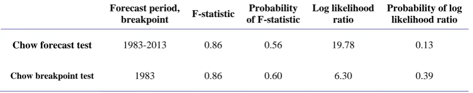
Table 7. Statistical output for stability test

Forecast period,

breakpoint F-statistic

Probability of F-statistic

Log likelihood ratio

Probability of log likelihood ratio

Chow forecast test 1983-2013 0.86 0.56 19.78 0.13

Chow breakpoint test 1983 0.86 0.60 6.30 0.39

Source: Research findings

Conclusion

The impacts of environmental performance index, foreign direct investment, and trade liberalization on economic growth of selected developing countries were reviewed throughout 1983–2013. The panel unit root tests, the bounds test (ARDL), and the diagnostic tests were employed in the present study.

According to the findings, a co-integration exists among the variables determined in the model given economic growth as the dependent variable. The economic growth is positively and significantly impacted by trade openness at a level of 5% as revealed by estimated long-run relationship coefficients. Accordingly, economic growth rises almost 0.05% by a 1% increase in trade openness, which corroborates those of Coe and Helpman (1995), Grossman and Helpman (1991), and Romer (1994).

Moreover, results indicated a positive and significant impact of environmental performance index on economic growth. Based on a magnitude of 1.51, economic growth will improve approx. 1.51% by a 1% rise in environmental performance index, which is consistent with Grossman and Krueger (1991), Shafik (1994), Aldy (2005), Song et al. (2008), and Iwata et al. (2009). Lastly, our findings reveal positive confirmation and significance of foreign direct investment variable, which agrees with Chakraborty (2001), Borensztein and Lee (1998), and De Mello (1997).

References

Acharyya, J. (2009). FDI, growth and the environment: evidence from India on Co2 emission during the last two decades. Journal of Economic Development, 34, 43–58.

Bhagwati, J.N. (1978). Foreign trade regimes and economic development: Anatomy and consequences of exchange control regime. Cambridge, MA: Ballinger.

Borensztein, E., De Gregorio, J., and Lee, J.W. (1998). How does foreign direct investment affect economic growth? Journal of International Economics, 45, 115-135.

Boyd, J.H. and Smith, B.D. (1992). Intermediation and the equilibrium allocation of investment capital: implications for economic development. Journal of Monetary Economics, 30, 409–432. Chakrabarti, A. (2001). The determinants of foreign direct investment: sensitivity analyses of

cross-country regressions. KYKLOS, 54, 89–114.

Christopher, O.O. and Douglason, G.O. (2011). Environmental quality and economic growth: Searching for environmental Kuznets curves for air and water pollutants in Africa. Energy Policy, 39, 4178–4188.

Coe, D.T. and Helpman, E. (1995). International R&D spillovers. European Economic Review, 39, 859–887.

De Mello, L.R. (1997). Foreign direct investment in developing countries: a selective survey. Journal of Development Studies, 34(1), 1–34.

De Mello Jr. and L.R. (1999). Foreign direct investment-led growth evidence from time series and panel data. Oxford Economics Papers, 51(2), 133–151.

Edwards, S. (1998). Openness, productivity and growth: What do we really know? The Economic Journal, 108, 383–398.

Friedl, B. and Getzner, M. (2003). Determinants of CO2 emissions in a small open economy. Ecological Economics, 45(1), 133–148.

Friedl, B. and Getzner, M. (2003). Determinants of CO2 emissions in a small open economy. Ecological Economics, 45(1), 133–148.

Grossman, G.M. and Helpman, E. (1991). Trade, knowledge spillovers, and growth. European Economic Review, 35, 517–526.

Grossman, G. and Krueger, A.B. (1991). Environmental Impact of a North American Free Trade Agreement. Combridge, National Bureau of Economic Research Working Paper.

Haussmann, R., Hwang, J. and Rodrik, D. (2007). What you export matters. Journal of Economic Growth, 12, 1–25.

Holtz-Eakin, D. and Selden, T.M. (1995). Stoking the fires?: CO2 emissions and economic growth. Journal of Public Economics, 57, 85–101.

Iwata, H., Okada, K. and Samreth, S. (2010). Empirical study on the environmental Kuznets curve for CO2 in France: the role of nuclear energy. Energy Policy, 38, 4057–4063.

Im, K.S., Pesaran, M.H. and Shin, Y. (2003). Testing for unit roots in heterogeneous panels.Journal of Econometrics, 115, 53-74.

Krueger, A.O. (1978). Foreign trade regimes and economic development: Liberalization attempts and consequences. Cambridge, MA: Ballinger.

Lau, L.S., Chong, C.K. and Eng, Y.K. (2014). Investigation of the environmental Kuznets curve for carbon emissions in Malaysia: do foreign direct investment and trade matter?. Energy Policy, 68, 490–497.

Levin, A., Linb, C. F. and James, C.S.J. (2002). Unit root tests in panel data: asymptotic and finite-sample properties. Journal of Econometrics, 108, 1–24.

Managia, Sh. and Jena, P.R. (2008). Environmental productivity and Kuznets curve in India. Ecological Economics, 65, 432-440.

Morley, B. (2006). Causality between economic growth and migration: an ARDL bounds testing approach. Economics Letters, 90, 72–76.

Narayan, P.K. and Smyth, R. (2006). Higher education, real income and real investment in China: evidence from Granger causality tests. Education Economics, 14(2), 107–125.

Narayan, P.K. and Smyth, R. (2008). Energy consumption and real GDP in G7 countries: new evidence from panel cointegration zith structural breaks. Energy Economics, 30(4), 2331–2341. Nazlioglu, S. and Soytas, U. (2012). Oil price, agricultural commodity prices, and the dollar: A panel

cointegration and causality analysis.Energy Economics, 34, 1098-1104.

Odhiambo, N.M. (2009). Energy consumption and economic growth in Tanzania: an ARDL bounds testing approach. Energy Policy, 37(2), 617–622.

Omri, A. (2013). CO2 emissions, energy consumption and economic growth nexus in MENA countries: evidence from simultaneous equations models. Energy Economics, 40, 657–664.

Omri, A., Khuong, N. D. and Rault, C. (2014). Causal interactions between CO2 emissions, FDI, and economic growth: Evidence from dynamic simultaneous-equation models. Original Research Article Economic Modeling, 42, 382–389.

Pesaran, M.H., Shin, Y. and Smith, R.J. (2001). Bounds testing approaches to the analysis of level relationship. Journal of Applied Economics, 16(1), 289–326.

Pesaran, M. and Shin, Y. (1999). An autoregressive distributed lag-modeling approach to cointegration analysis. In: Strom, S. (Ed.), Econometrics and Economic Theory in the 20th Century: The Ragnar Frisch Centennial Symposium. Cambridge University Press, Cambridge. Richmond, A.K. and Kaufmann, R.K. (2006). Is there a turning point in the relationship between

income and energy use and/or carbon emissions?. Ecological Economics, 56, 176–189.

Song, T., Zheng, T. and Tong, L. (2008). An empirical test of the environmental Kuznets curve in China: A panel cointegration approach. China Economic Review, 19, 381–392.

Shafik, N. (1994). Economic development and environmental quality: an econometric analysis. Oxford Economic Papers, 46, 757–773.

Zhang, Y.J. (2011). The impact of financial growth on carbon emissions: an empirical analysis in China. Energy Policy, 39, 2197–2203.